
Development of a Distributed Mathematical Model and Control System for Reducing Pollution Risk in Mineral Water Aquifer Systems


Abstract
:1. Introduction
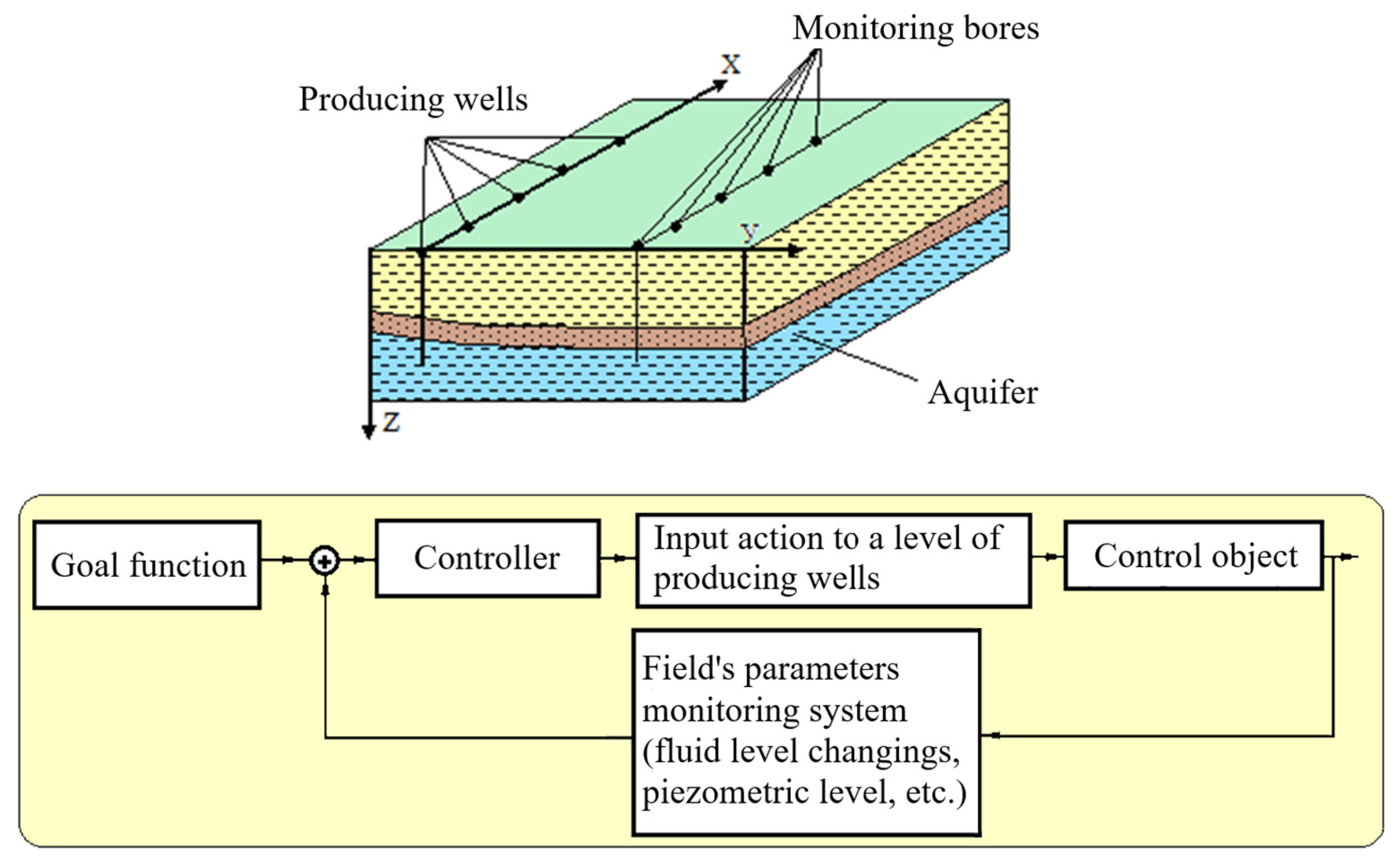
2. Problem Statement
- Possibility of considering the spatial distribution of the object (field);
- Modeling a complex of interconnected hydrogeological objects;
- Ability to control the parameters of the operating mode of a group of hydrogeological objects.
3. Methods
3.1. Method Description
- First group. Deposits with a simple geological structure containing large or medium-sized bodies of minerals, which can be characterized by the stable thickness and internal structure, consistent quality of minerals and uniform distribution of the main valuable components.
- Second group. Deposits with a complex geological structure containing large and medium-sized bodies with disturbed bedding, which can be characterized by unstable thickness and uneven distribution of the main valuable components.
- Third group. Deposits with a very complex geological structure containing medium and small-sized bodies of minerals with intensively disturbed occurrence, which can be characterized by very variable thickness and internal structure, and a very uneven distribution of the main valuable components.
- Fourth group. Deposits with a small, less often medium-sized bodies containing extremely disturbed bedding, which can be characterized by sharp variability of thickness and internal structure, extremely uneven quality of the mineral [18].
- Delphi 7 software package;
- Software package for modeling hydrodynamic processes developed up to GOST R 57,700.2;
- Software package for modeling parameters of an open-loop control system developed up to GOST 24.104-85;
- A software package for modeling the parameters of a closed-loop control system developed up to GOST 24.104-85;
- A software package for modeling the spatial heterogeneity of the field strata hydrogeological structure developed up to GOST R 57,700.2 [21].
- Hydrogeological conditions (lithological structure of water-bearing soils, feeding characteristics and conditions at the boundaries of the tested layer);
- Groundwater regime (features of the pressure fluctuations nature—levels and the influence on these fluctuations of various disturbing sources, including technogenic);
- Technological conditions for testing, the data of which are used to check the accuracy of modeling (fluctuations in flow rate and pressure during pumping) [28].
3.2. Development of the “Reservoir” Layout
- DBGrid (for the “temperature” table displaying);
- DBNavigator (for table entries managing);
- ADOConnection (for the communication with the database);
- ADOQwery;
- ComPortDriver;
- Timer;
- DataSource.
4. Development of an Experimental Reservoir’s Distributed Mathematical Model
- The proposed method takes into account the interstratal interactions of aquifer;
- The proposed method gives a possibility of a three-dimensional model of the field mathematical description;
- The proposed method provides a sufficiently high accuracy of the hydrodynamic processes’ reflection for a given experiment;
- The proposed method was successfully tested at one of the fields in the region under consideration [3].
5. Results
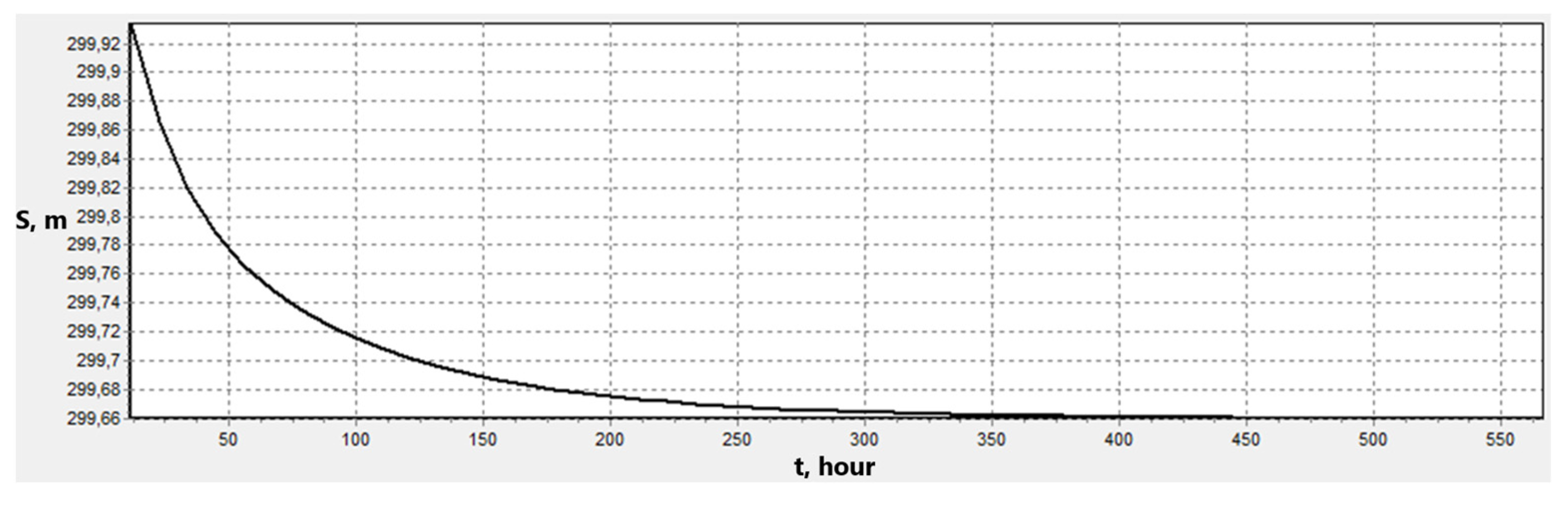
5.1. Method Effectiveness Analysis
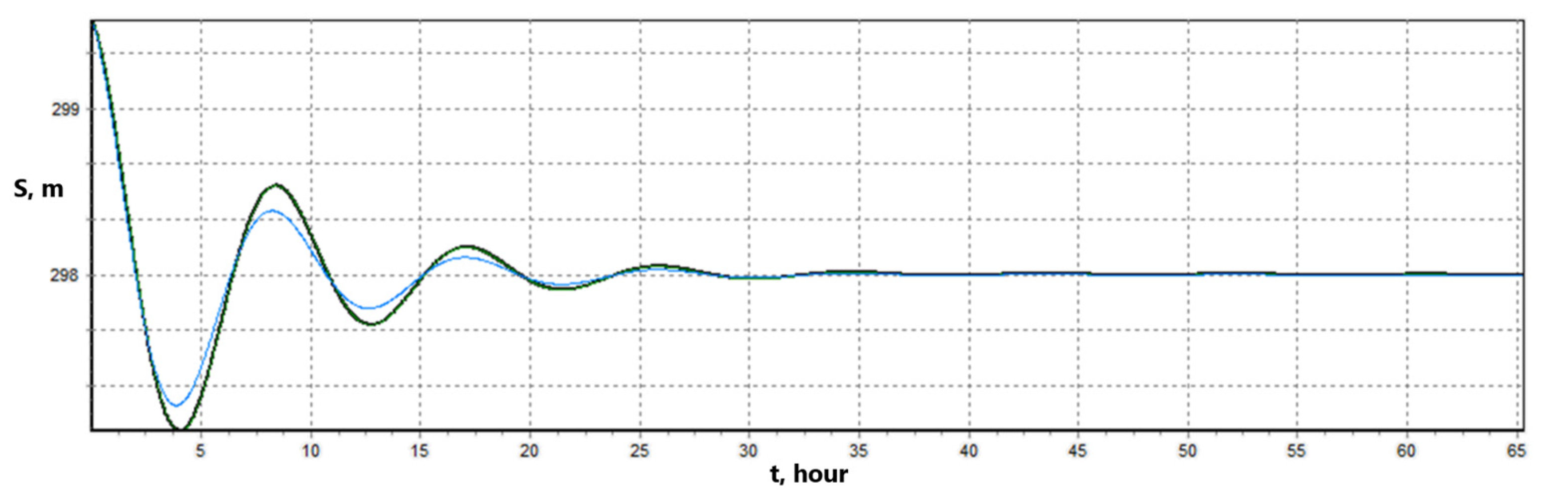
5.2. Control System Synthesis Results
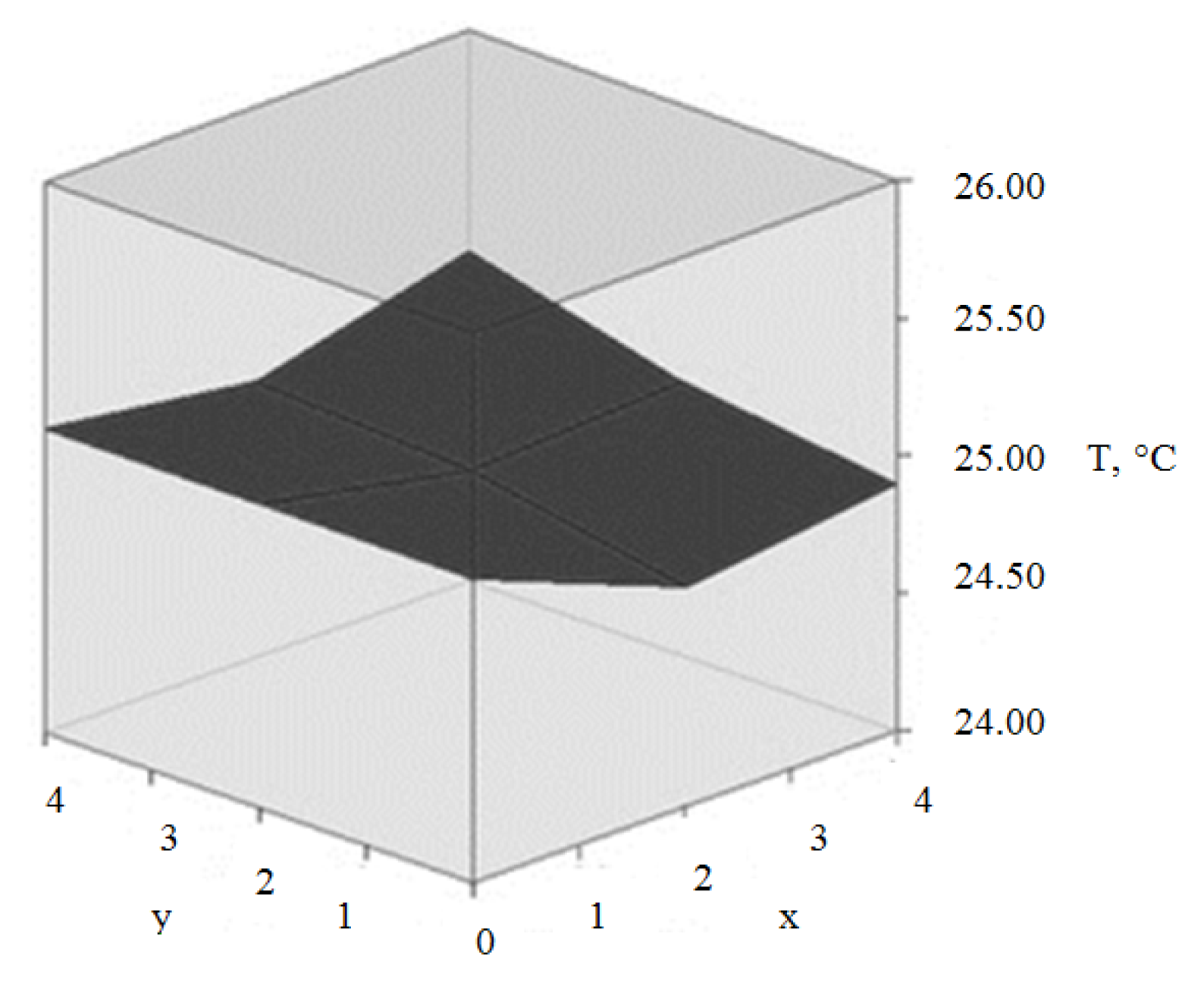
5.3. Experimental Reservoir’s Distributed Mathematical Model Result Analysis
6. Conclusions
- Application of sensitivity analysis methods to assess the impact of changes in the initial parameters of the model on the output characteristics.
- Adaptation and scaling of the developed modeling methods for solving problems of the oil and gas industry.
Author Contributions
Funding
Data Availability Statement
Conflicts of Interest
References
- Resniova, E.; Ponomarenko, T. Sustainable Development of the Energy Sector in a Country Deficient in Mineral Resources: The case of the Republic of Moldova. Sustainability 2021, 13, 3261. [Google Scholar] [CrossRef]
- Ponomarenko, T.; Nevskaya, M.; Jonek-Kowalska, I. Mineral Resource Depletion Assessment: Alternatives, problems, results. Sustainability 2021, 13, 862. [Google Scholar] [CrossRef]
- Pershin, I.M.; Malkov, A.V.; Pomelyayko, I.S. Design of a distributed debit management network of operating wells of fields of the CMW region. In Proceedings of the 3rd International Conference on Futuristic Trends in Network and Communication Technologies, Taganrog, Russia, 14–16 October 2020; pp. 317–328. [Google Scholar]
- Vasilev, Y.; Cherepovitsyn, A.; Tsvetkova, A.; Komendantova, N. Promoting Public Awareness of Carbon Capture and Storage Technologies in the Russian Federation: A system of educational activities. Energies 2021, 14, 1408. [Google Scholar] [CrossRef]
- Pershin, I.M.; Kukharova, T.V.; Tsapleva, V.V. Designing of Distributed Systems of Hydrolithosphere Processes Parameters Control for the Efficient Extraction of Hydromineral Raw Materials. J. Phys. Conf. Ser. 2021, 1728, 012017. [Google Scholar] [CrossRef]
- Pomelyaiko, I.S.; Malkov, A.V. Quality Problems of Surface Water and Groundwater at the Health Resorts in the Regions of Caucasian Mineral Waters and Ways to Their Solution. Water Resour. 2019, 46, 214–225. [Google Scholar] [CrossRef]
- Hirsch, R.M.; Slack, J.R.; Smith, R.A. Techniques of Trend Analysis for Monthly Water Quality Data. Water Resour. Res. 1982, 18, 107–121. [Google Scholar] [CrossRef] [Green Version]
- Hombeck, R.; Keskin, P. The evolving impact of the Ogallala Aquifer—Agricultural adaptation to groundwater and climate. US Natl. Bur. Econ. Res. Work. Pap. 2011, 39, 17625. [Google Scholar]
- Iverson, R.M. Landslide Triggering by Rain Infiltration. Water Resour. Res. 2000, 36, 1897–1910. [Google Scholar] [CrossRef] [Green Version]
- Jourabchi, P.; Lin, G.K.-C. Modeling Vapor Migration for Estimating the Time to Reach Steady State Conditions. Groundw. Monit. Remediat. 2021, 41, 25–32. [Google Scholar] [CrossRef]
- Zolotov, O.I.; Ilyushina, A.N.; Novozhilov, I.M. Spatially distributed system for monitoring of fields technical condition in mineral resources sector. In Proceedings of the XXIV International Conference on Soft Computing and Measurements, Saint-Petersburg, Russia, 26–28 May 2021; pp. 93–95. [Google Scholar]
- Xing, L.; Wen, C.; Liu, Z.; Su, H.; Cai, J. Event-Triggered Adaptive Control for a Class of Uncertain Nonlinear Systems. IEEE Trans. Fuzzy Syst. 2017, 62, 2071–2076. [Google Scholar] [CrossRef]
- Feng, G. A Survey on Analysis and Design of Model-Based Fuzzy Control Systems. IEEE Trans. Fuzzy Syst. 2006, 14, 676–697. [Google Scholar] [CrossRef] [Green Version]
- Hou, Z.; Xiong, S. On Model-Free Adaptive Control and Its Stability Analysis. IEEE Trans. Autom. Control 2019, 64, 4555–4569. [Google Scholar] [CrossRef]
- Hu, X.; Li, Y.; Che, X.; Hou, Z. Event-Based Adaptive Fuzzy Asymptotic Tracking Control of Uncertain Nonlinear Systems. IEEE Trans. Fuzzy Syst. 2021, 29, 3003–3013. [Google Scholar]
- Golubev, V.O.; Litvinova, T.E. Dynamic simulation of industrial-scale gibbsite crystallization circuit. J. Min. Inst. 2021, 247, 88–101. [Google Scholar] [CrossRef]
- Tavernini, D.; Metzler, M.; Gruber, P.; Sorniotti, A. Explicit Nonlinear Model Predictive Control for Electric Vehicle Traction Control. IEEE Trans. Control Syst. Technol. 2019, 27, 1438–1451. [Google Scholar] [CrossRef]
- Guidelines on Alignment of Russian Minerals Reporting Standards and the CRIRSCO Template. Available online: https://www.crirsco.com/docs/conversion_guidelines_final.pdf (accessed on 17 December 2021).
- Federal Agency of Technical Control and Metrology. GOST 23278–78. Available online: http://protect.gost.ru/document1.aspx?control=31&baseC=6&page=0&month=5&year=2017&search=23278&id=188687 (accessed on 15 November 2021).
- Federal Agency of Technical Control and Metrology. GOST R 57700.2. Available online: http://protect.gost.ru/document1.aspx?control=31&baseC=6&page=4&month=5&year=2017&search=&id=217662 (accessed on 15 November 2021).
- Dashko, R.E.; Romanov, I.S. Forecasting of Mining and Geological Processes Based on the Analysis of the Underground Space of the Kupol Field as a Multicomponent System. J. Min. Inst. 2021, 247, 20–32. [Google Scholar] [CrossRef]
- Khabarov, N.; Smirnov, A.; Balkovič, J.; Skalský, R.; Folberth, C.; Van Der Velde, M.; Obersteiner, M. Heterogeneous Compute Clusters and Massive Environmental Simulations Based on the EPIC Model. Modelling 2020, 1, 215–224. [Google Scholar] [CrossRef]
- Korotenko, V.A.; Grachev, S.I.; Kushakova, N.P.; Mulyavin, S.F. Assessment of the Influence of Water Saturation and Capillary Pressure Gradients on Size Formation Of Two-Phase Filtration Zone in Compressed Low-permeable Reservoir. J. Min. Inst. 2020, 245, 569–581. [Google Scholar] [CrossRef]
- Reinecke, R.; Wachholz, A.; Mehl, S.; Foglia, L.; Niemann, C.; Döll, P. Importance of Spatial Resolution in Global Groundwater Modeling. Groundwater 2020, 58, 363–376. [Google Scholar] [CrossRef] [Green Version]
- Meshkov, A.A.; Kazanin, O.I.; Sidorenko, A.A. Improving the Efficiency of the Technology and Organization of the Longwall Face Move During the Intensive Flat-lying Coal Seams Mining at the Kuzbass Mines. J. Min. Inst. 2021, 249, 342–350. [Google Scholar] [CrossRef]
- Kupfersberger, H.; Rock, G.; Draxler, J.C. Combining Groundwater Flow Modeling and Local Estimates of Extreme Groundwater Levels to Predict the Groundwater Surface with a Return Period of 100 Years. Geosciences 2020, 10, 373. [Google Scholar] [CrossRef]
- Metzler, M.; Tavernini, D.; Gruber, P.; Sorniotti, A. On Prediction Model Fidelity in Explicit Nonlinear Model Predictive Vehicle Stability Control. IEEE Trans. Control Syst. Technol. 2021, 29, 1964–1980. [Google Scholar] [CrossRef]
- Klizas, P. Geofiltration studies of clay at the future radioactive waste repository for Ignalina nuclear power plant. J. Environ. Eng. Landsc. Manag. 2021, 22, 219–225. [Google Scholar] [CrossRef] [Green Version]
- Pashkevich, N.V.; Golovina, E.I. Topical issues of the management of extraction of underground waters on the territory of the Russian Federation. J. Min. Inst. 2014, 210, 99–107. [Google Scholar]
- Takemura, J.; Yao, C.; Kusakabe, O. Development of a Fault Simulator for Soils under Large Vertical Stress in a Centrifuge. Int. J. Phys. Model. Geotech. 2020, 20, 118–131. [Google Scholar] [CrossRef]
- Martirosyan, A.; Martirosyan, K. Quality improvement information technology for mineral water field’s control. In Proceedings of the IEEE Conference on Quality Management, Transport and Information Security, Information Technologies, Nalchik, Russia, 4–11 October 2016; pp. 147–151. [Google Scholar]
- Jensen, J.K.; Nilsson, B.; Engesgaard, P. Numerical Modeling of Nitrate Removal in Anoxic Groundwater during River Flooding of Riparian Zones. Groundwater 2021, 59, 866–877. [Google Scholar] [CrossRef] [PubMed]
- Qin, H. Numerical groundwater modeling and scenario analysis of Beijing plain: Implications for sustainable groundwater management in a region with intense groundwater depletion. Environ. Earth Sci. 2021, 80, 499. [Google Scholar] [CrossRef]
- Medici, G.; Smeraglia, L.; Torabi, A.; Botter, C. Review of Modeling Approaches to Groundwater Flow in Deformed Carbonate Aquifers. Groundwater 2021, 59, 334–351. [Google Scholar] [CrossRef]
- Ou, G. Development of GUI Applications for Groundwater Modeling Using Python. Groundwater 2020, 58, 496–497. [Google Scholar] [CrossRef]
- Ilyushina, A.N.; Novozhilov, I.M. Development of the automated temperature field control system with a pulsed heating source. In Proceedings of the III International Conference on Control in Technical Systems, Saint-Petersburg, Russia, 30 October–1 November 2019; pp. 160–163. [Google Scholar]
- Cao, Z.; Niu, Y.; Lam, H.-K.; Zhao, J. Sliding Mode Control of Markovian Jump Fuzzy Systems: A Dynamic Event-Triggered Method. IEEE Trans. Fuzzy Syst. 2021, 29, 2902–2915. [Google Scholar] [CrossRef]


| Water Name | Mineralization g/dm3 | Main Ionic Composition | Bioactive Agents | |||||
|---|---|---|---|---|---|---|---|---|
| Anions, mg/dm3 | Cations, mg/dm3 | |||||||
| HCO3− | SO42− | Cl− | Ca2+ | Mg2+ | (Na+ + K+) | |||
| Narzan | 2.0–3.5 | 1000–1700 | 250–500 | 50–200 | 200–500 | 50–150 | 50–250 | CO2 1000–2500 |
| Dolomitic Narzan | 4.0–4.5 | 2000–2300 | 600–800 | 250–350 | 650–700 | 100–180 | 300–400 | CO2 2000–2300 |
| Sulphatic Narzan | 5.0–5.5 | 2300–2500 | 1400–1600 | <50 | 700–800 | 200–400 | 200–300 | CO2 2000–2300 |
| Essentuki 4 | 7.0–10.0 | 3400–4800 | <25 | 1300–2000 | <150 | <100 | 2000–3000 | H3BO3 30–60, CO2 500–1800 |
| Essentuki 17 | 10.0–14.0 | 5000–7200 | <150 | 1200–2200 | <150 | <150 | 2700–3900 | H3BO3 30–80, CO2 500–1200 |
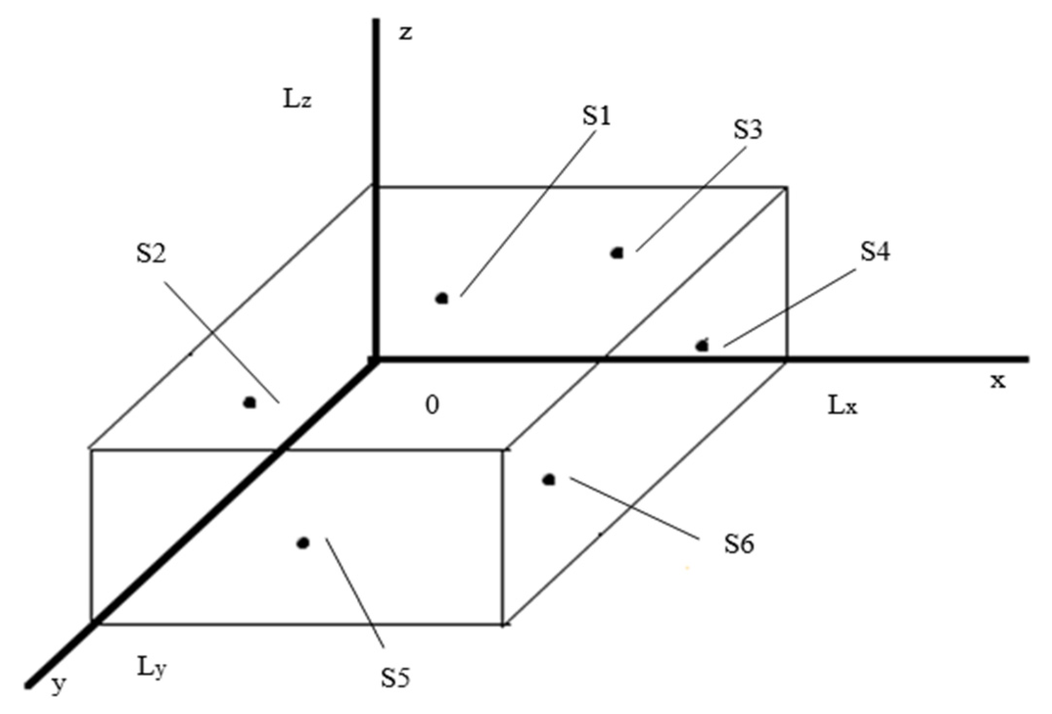
| LX, m | LY, m | LZ, m | ∂, t s. | S1 | S2 | S3 | S4 | S5 | S6 |
|---|---|---|---|---|---|---|---|---|---|
| 0.03 | 0.03 | 0.01 | 1 | 0 | 0 | 0 | 0 | 0 | 0 |
Publisher’s Note: MDPI stays neutral with regard to jurisdictional claims in published maps and institutional affiliations. |
© 2022 by the authors. Licensee MDPI, Basel, Switzerland. This article is an open access article distributed under the terms and conditions of the Creative Commons Attribution (CC BY) license (https://creativecommons.org/licenses/by/4.0/).
Share and Cite
Martirosyan, A.V.; Ilyushin, Y.V.; Afanaseva, O.V. Development of a Distributed Mathematical Model and Control System for Reducing Pollution Risk in Mineral Water Aquifer Systems. Water 2022, 14, 151. https://doi.org/10.3390/w14020151
Martirosyan AV, Ilyushin YV, Afanaseva OV. Development of a Distributed Mathematical Model and Control System for Reducing Pollution Risk in Mineral Water Aquifer Systems. Water. 2022; 14(2):151. https://doi.org/10.3390/w14020151
Chicago/Turabian StyleMartirosyan, Alexander V., Yury V. Ilyushin, and Olga V. Afanaseva. 2022. "Development of a Distributed Mathematical Model and Control System for Reducing Pollution Risk in Mineral Water Aquifer Systems" Water 14, no. 2: 151. https://doi.org/10.3390/w14020151