

Comparative Evaluation of Five Hydrological Models in a Large-Scale and Tropical River Basin
 , , ,
, , ,
Abstract
:1. Introduction
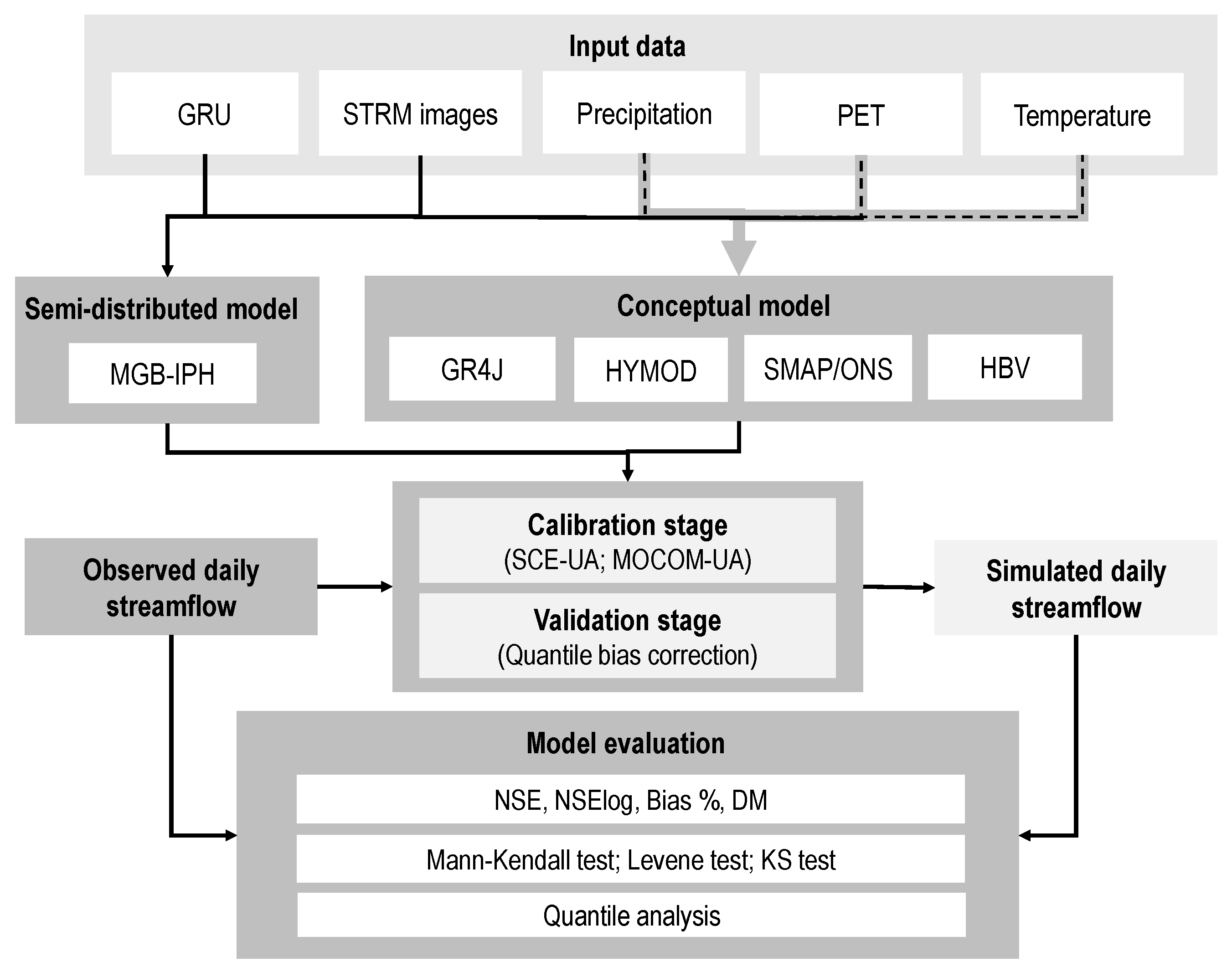
2. Methodology
2.1. HYMOD Model
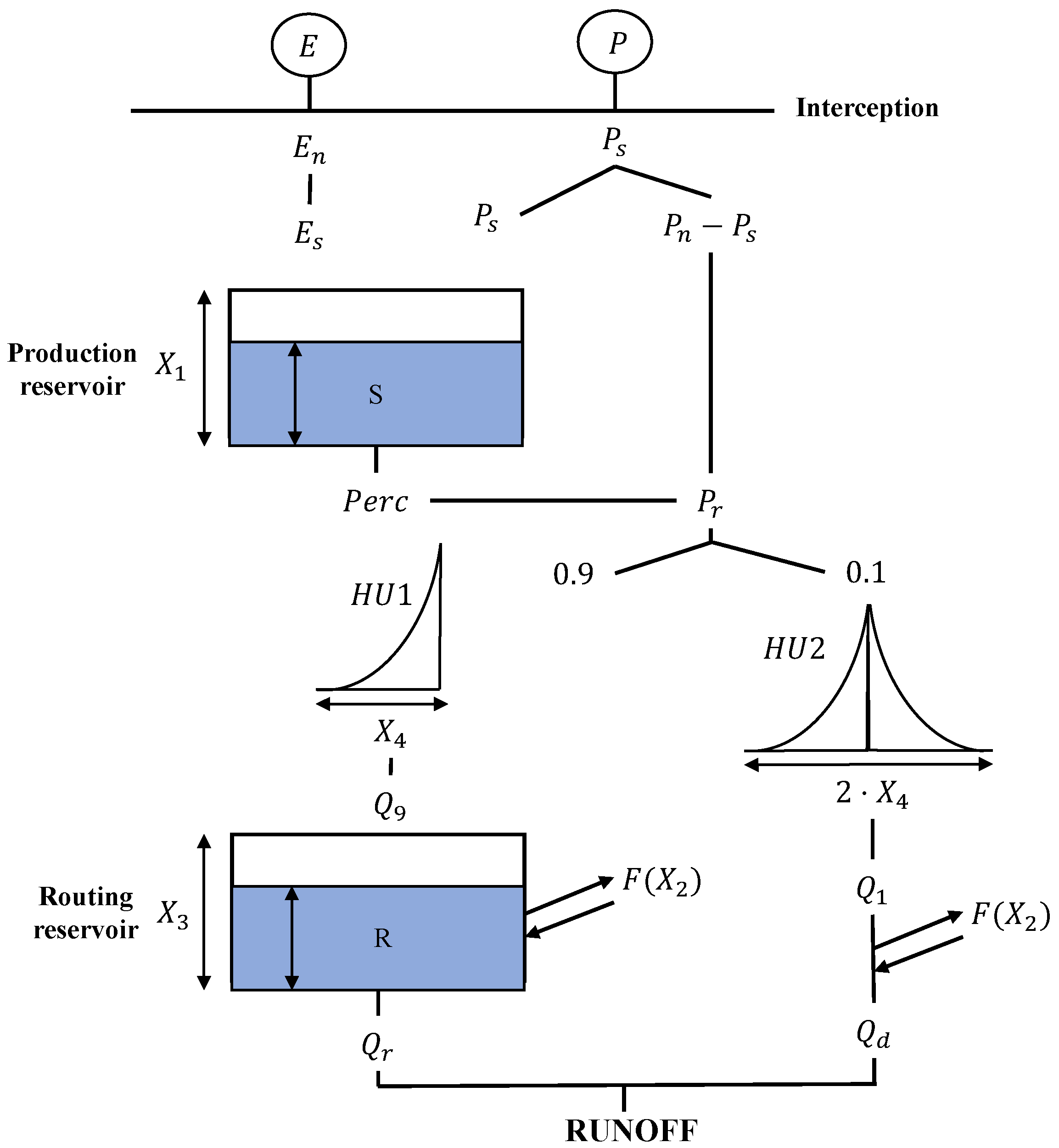
2.2. GR4J Model
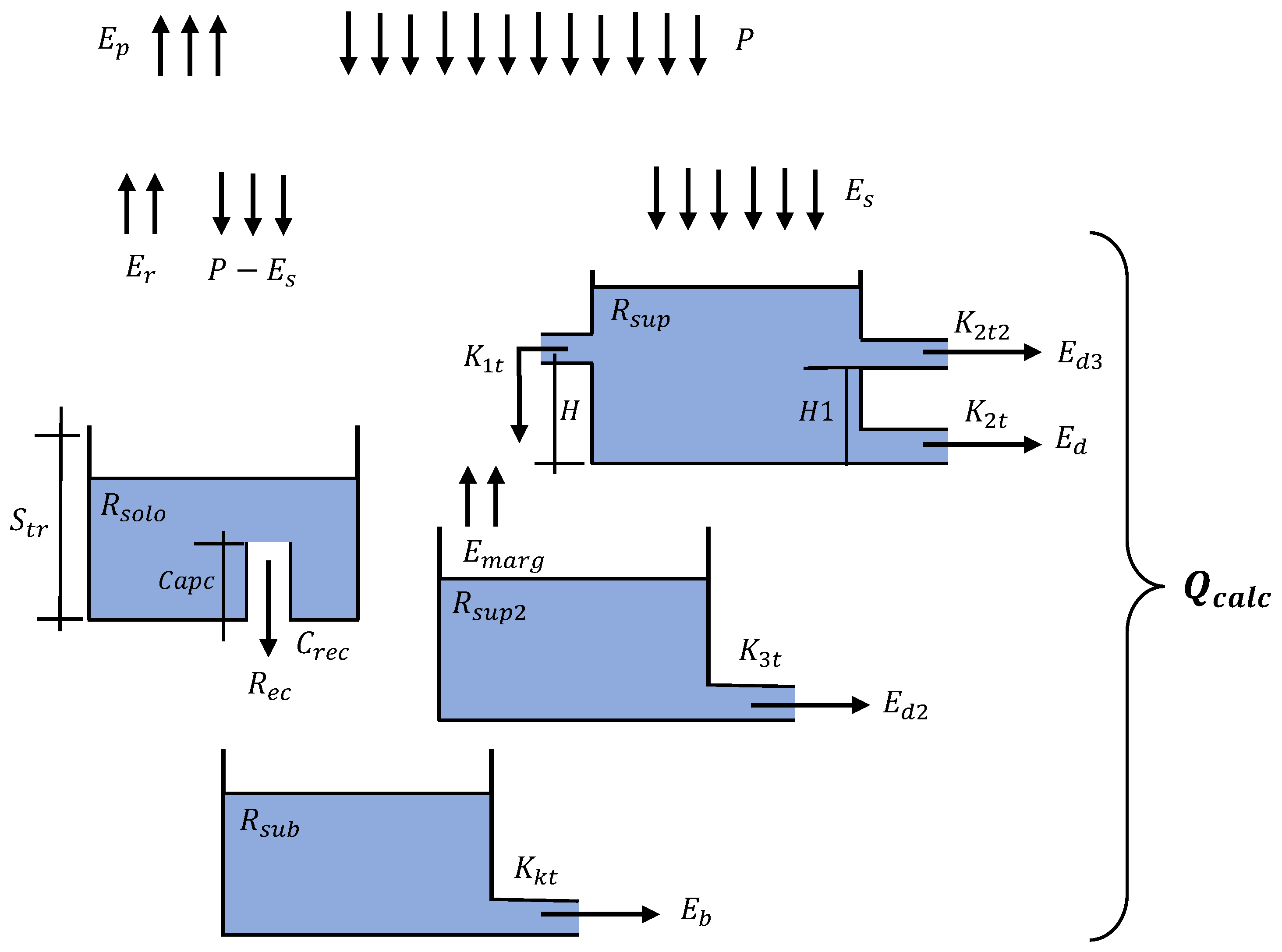
2.3. SMAP Model
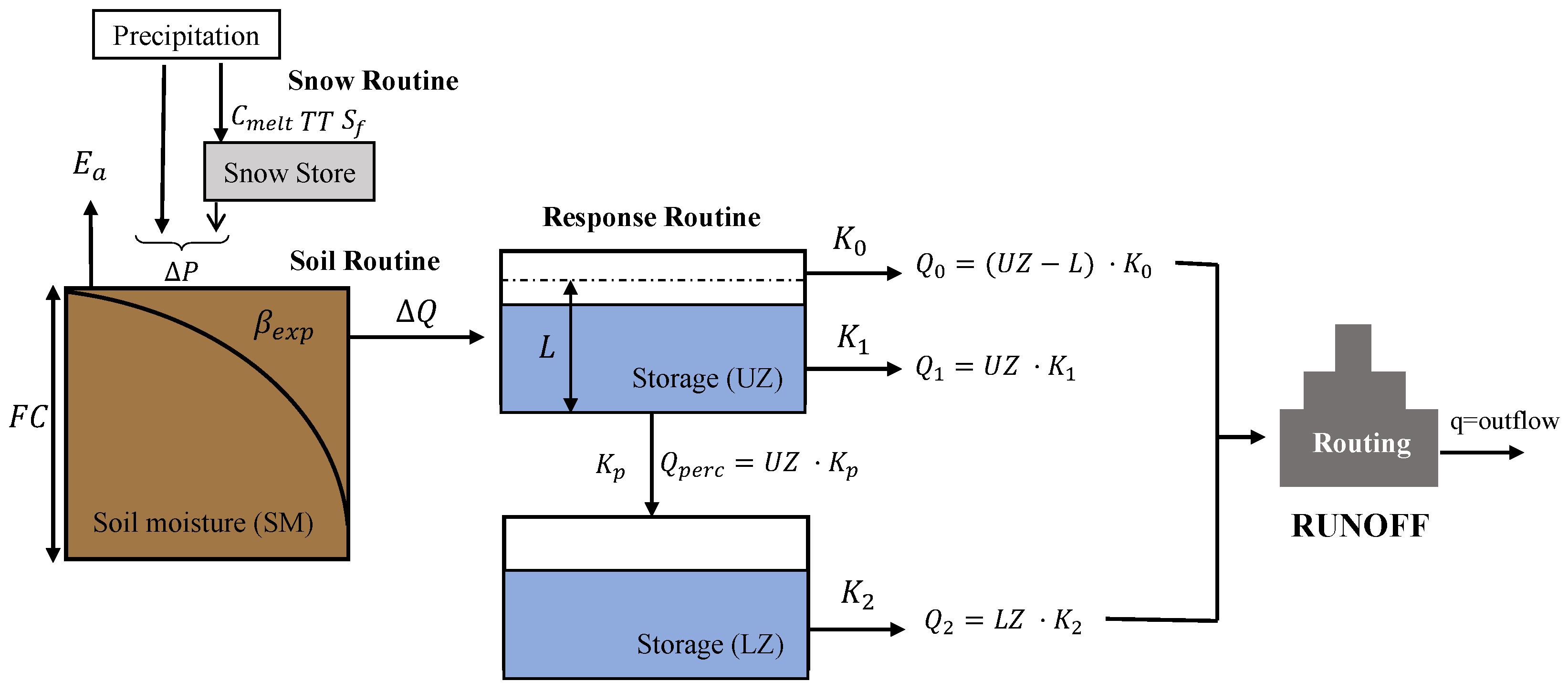
2.4. HBV Model
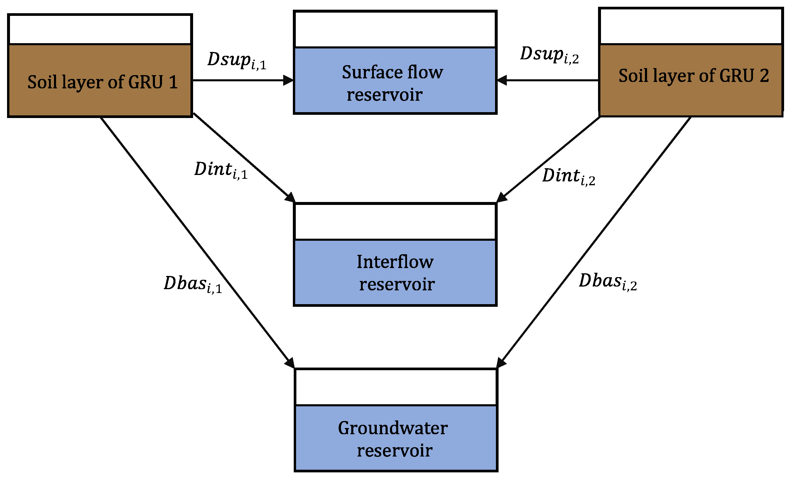
2.5. MGB-IPH Model
2.6. Performance Metrics
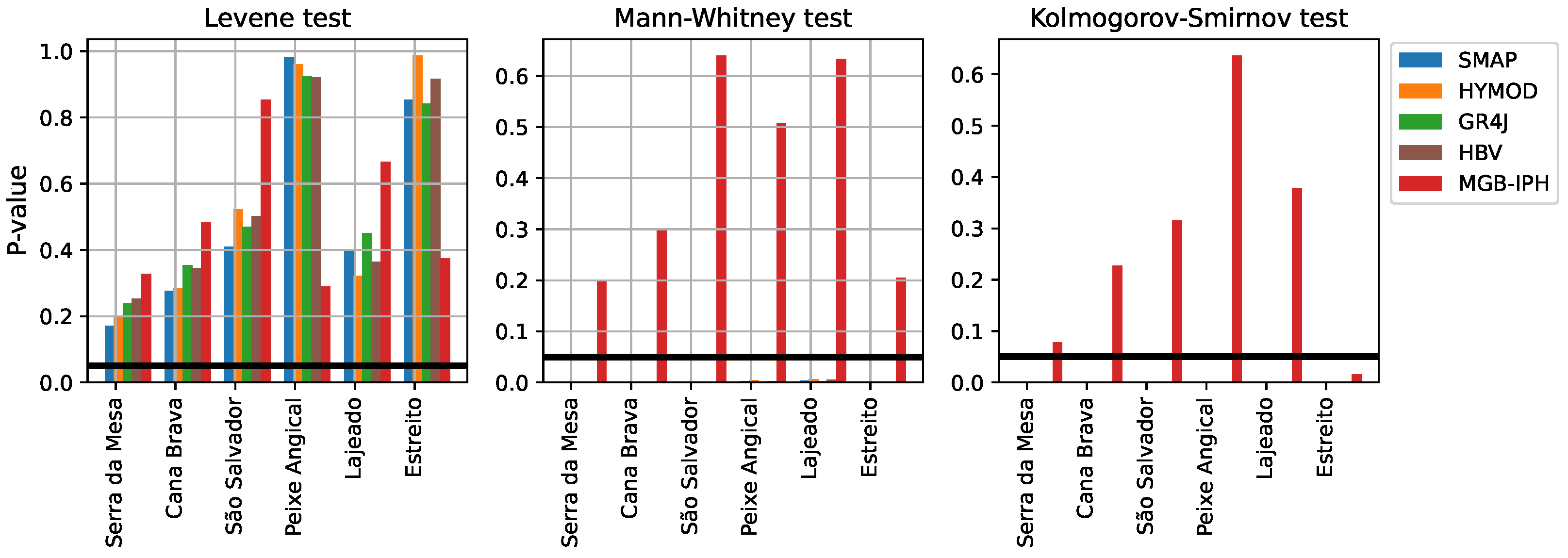
2.7. Statistical Tests
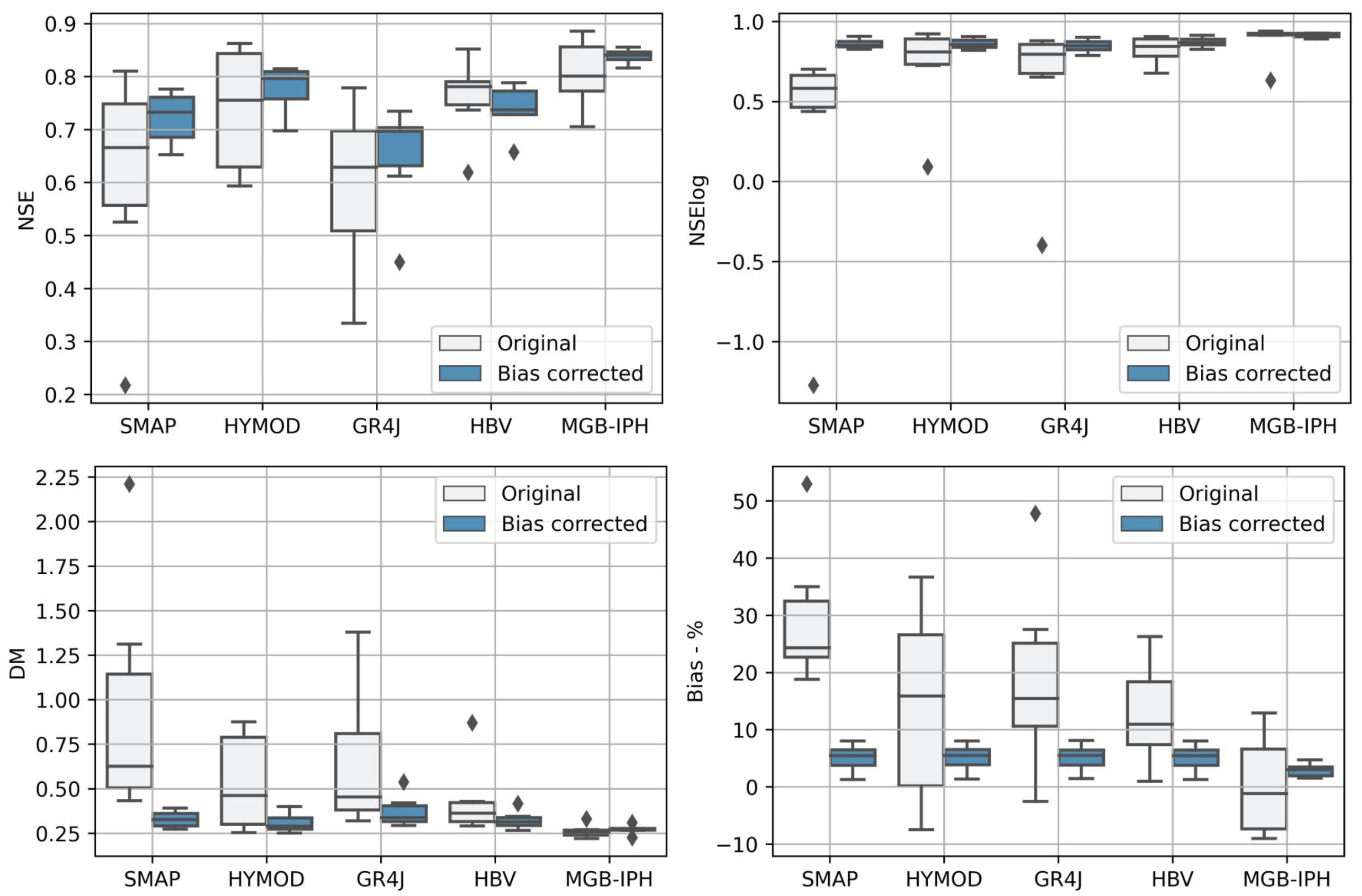
2.8. Bias Correction
3. Case Study
3.1. Overview
3.2. Data
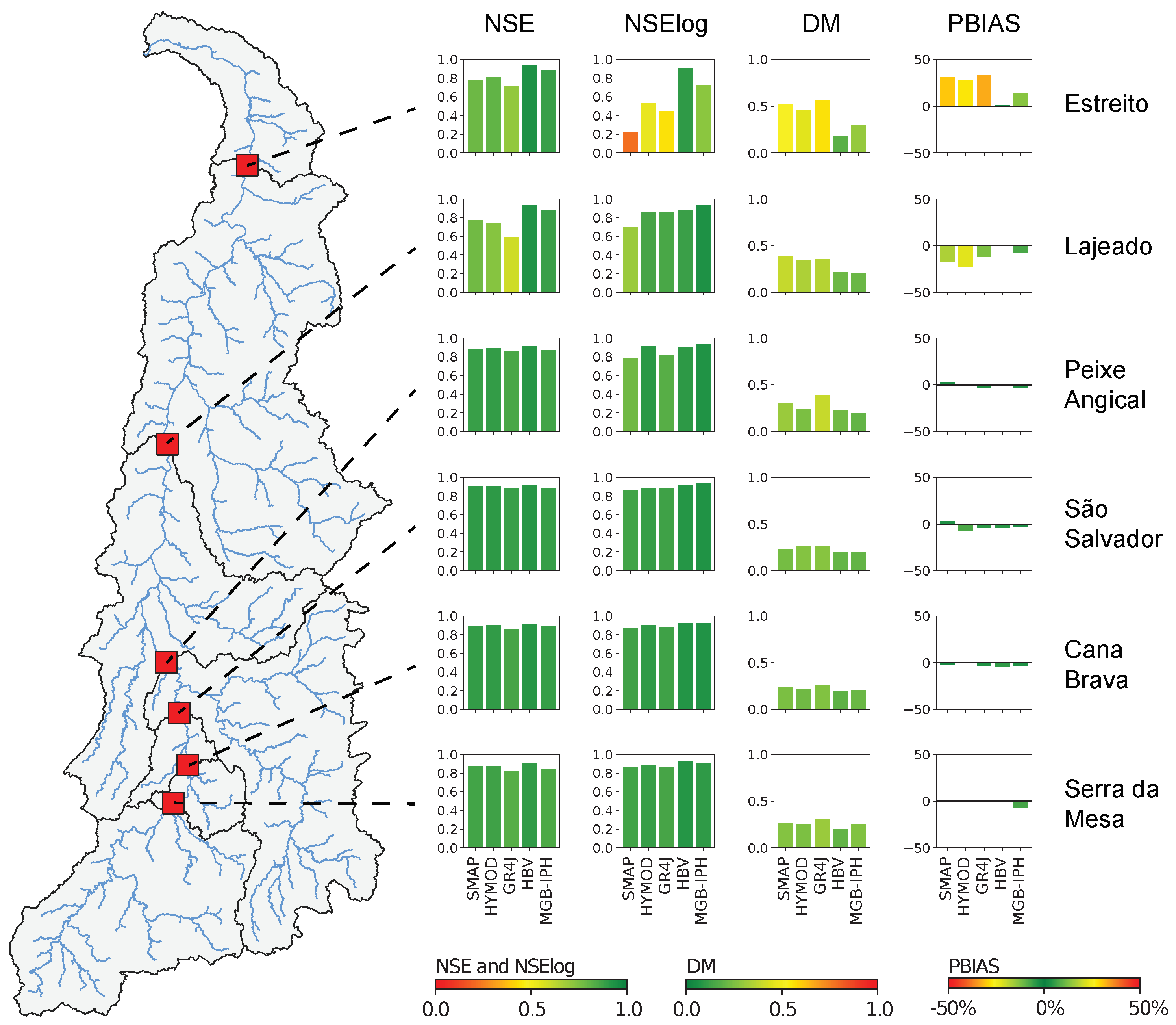
3.3. Results Analysis
4. Conclusions
Author Contributions
Funding
Data Availability Statement
Acknowledgments
Conflicts of Interest
References
- Coulibaly, P.; Anctil, F.; Bobée, B. Daily reservoir inflow forecasting using artificial neural networks with stopped training approach. J. Hydrol. 2000, 230, 244–257. [Google Scholar] [CrossRef]
- Zhang, D.; Peng, Q.; Lin, J.; Wang, D.; Liu, X.; Zhuang, J. Simulating reservoir operation using a recurrent neural network algorithm. Water 2019, 11, 865. [Google Scholar] [CrossRef]
- Yang, S.; Yang, D.; Chen, J.; Zhao, B. Real-time reservoir operation using recurrent neural networks and inflow forecast from a distributed hydrological model. J. Hydrol. 2019, 579, 124229. [Google Scholar] [CrossRef]
- Zhao, T.; Cai, X.; Yang, D. Effect of streamflow forecast uncertainty on real-time reservoir operation. Adv. Water Resour. 2011, 34, 495–504. [Google Scholar] [CrossRef]
- Koneti, S.; Sunkara, S.L.; Roy, P.S. Hydrological modeling with respect to impact of land-use and land-cover change on the runoff dynamics in Godavari River Basin using the HEC-HMS model. ISPRS Int. J. Geo-Inf. 2018, 7, 206. [Google Scholar] [CrossRef]
- Krysanova, V.; Donnelly, C.; Gelfan, A.; Gerten, D.; Arheimer, B.; Hattermann, F.; Kundzewicz, Z.W. How the performance of hydrological models relates to credibility of projections under climate change. Hydrol. Sci. J. 2018, 63, 696–720. [Google Scholar] [CrossRef]
- Duan, Q.; Pappenberger, F.; Wood, A.; Cloke, H.L.; Schaake, J. Handbook of Hydrometeorological Ensemble Forecasting; Springer: Berlin/Heidelberg, Germany, 2019. [Google Scholar]
- Devia, G.K.; Ganasri, B.; Dwarakish, G. A review on hydrological models. Aquat. Procedia 2015, 4, 1001–1007. [Google Scholar] [CrossRef]
- Darbandsari, P.; Coulibaly, P. Inter-comparison of lumped hydrological models in data-scarce watersheds using different precipitation forcing data sets: Case study of Northern Ontario, Canada. J. Hydrol. Reg. Stud. 2020, 31, 100730. [Google Scholar] [CrossRef]
- Wheater, H.; Jakeman, A.; Beven, K. Progress and Directions in Rainfall-Runoff Modelling; John Wiley and Sons Ltd.: Hoboken, NJ, USA, 1993. [Google Scholar]
- Pechlivanidis, I.; Jackson, B.; Mcintyre, N.; Wheater, H. Catchment scale hydrological modelling: A review of model types, calibration approaches and uncertainty analysis methods in the context of recent developments in technology and applications. Glob. NEST J. 2011, 13, 193–214. [Google Scholar]
- Dawson, C.W.; Abrahart, R.J.; Shamseldin, A.Y.; Wilby, R.L. Flood estimation at ungauged sites using artificial neural networks. J. Hydrol. 2006, 319, 391–409. [Google Scholar] [CrossRef]
- Freire, P.K.d.M.M.; Santos, C.A.G.; da Silva, G.B.L. Analysis of the use of discrete wavelet transforms coupled with ANN for short-term streamflow forecasting. Appl. Soft Comput. 2019, 80, 494–505. [Google Scholar] [CrossRef]
- Camacho, F.; McLeod, A.I.; Hipel, K.W. Contemporaneous autoregressive-moving average (CARMA) modeling in water resources 1. JAWRA J. Am. Water Resour. Assoc. 1985, 21, 709–720. [Google Scholar] [CrossRef]
- Hao, Z.; Singh, V.P. Review of dependence modeling in hydrology and water resources. Prog. Phys. Geogr. 2016, 40, 549–578. [Google Scholar] [CrossRef]
- Chang, F.J.; Chang, Y.T. Adaptive neuro-fuzzy inference system for prediction of water level in reservoir. Adv. Water Resour. 2006, 29, 1–10. [Google Scholar] [CrossRef]
- Jaiswal, R.; Ali, S.; Bharti, B. Comparative evaluation of conceptual and physical rainfall–runoff models. Appl. Water Sci. 2020, 10, 1–14. [Google Scholar] [CrossRef]
- Beven, K.; Freer, J. Equifinality, data assimilation, and uncertainty estimation in mechanistic modelling of complex environmental systems using the GLUE methodology. J. Hydrol. 2001, 249, 11–29. [Google Scholar] [CrossRef]
- Shi, P.; Chen, C.; Srinivasan, R.; Zhang, X.; Cai, T.; Fang, X.; Qu, S.; Chen, X.; Li, Q. Evaluating the SWAT model for hydrological modeling in the Xixian watershed and a comparison with the XAJ model. Water Resour. Manag. 2011, 25, 2595–2612. [Google Scholar] [CrossRef]
- Newman, A.J.; Clark, M.P.; Winstral, A.; Marks, D.; Seyfried, M. The use of similarity concepts to represent subgrid variability in land surface models: Case study in a snowmelt-dominated watershed. J. Hydrometeorol. 2014, 15, 1717–1738. [Google Scholar] [CrossRef]
- Liang, X.; Xie, Z. A new surface runoff parameterization with subgrid-scale soil heterogeneity for land surface models. Adv. Water Resour. 2001, 24, 1173–1193. [Google Scholar] [CrossRef]
- Guo, S.; Guo, J.; Zhang, J.; Chen, H. VIC distributed hydrological model to predict climate change impact in the Hanjiang basin. Sci. China Ser. E Technol. Sci. 2009, 52, 3234–3239. [Google Scholar] [CrossRef]
- Alvarenga, L.A.; de Mello, C.R.; Colombo, A.; Chou, S.C.; Cuartas, L.A.; Viola, M.R. Impacts of climate change on the hydrology of a Small Brazilian headwater catchment using the distributed hydrology-soil-vegetation model. Am. J. Clim. Chang. 2018, 7, 355. [Google Scholar] [CrossRef] [Green Version]
- Moreda, F.; Koren, V.; Zhang, Z.; Reed, S.; Smith, M. Parameterization of distributed hydrological models: Learning from the experiences of lumped modeling. J. Hydrol. 2006, 320, 218–237. [Google Scholar] [CrossRef]
- Kirkby, M.; Beven, K. A physically based, variable contributing area model of basin hydrology. Hydrol. Sci. J. 1979, 24, 43–69. [Google Scholar]
- Zhang, S.; Al-Asadi, K. Evaluating the effect of numerical schemes on hydrological simulations: HYMOD as a case study. Water 2019, 11, 329. [Google Scholar] [CrossRef]
- Clark, M.P.; Kavetski, D. Ancient numerical daemons of conceptual hydrological modeling: 1. Fidelity and efficiency of time stepping schemes. Water Resour. Res. 2010, 46. [Google Scholar] [CrossRef]
- Kavetski, D.; Clark, M.P. Ancient numerical daemons of conceptual hydrological modeling: 2. Impact of time stepping schemes on model analysis and prediction. Water Resour. Res. 2010, 46. [Google Scholar] [CrossRef]
- Fenicia, F.; Kavetski, D.; Savenije, H.H. Elements of a flexible approach for conceptual hydrological modeling: 1. Motivation and theoretical development. Water Resour. Res. 2011, 47. [Google Scholar] [CrossRef]
- Clark, M.P.; Slater, A.G.; Rupp, D.E.; Woods, R.A.; Vrugt, J.A.; Gupta, H.V.; Wagener, T.; Hay, L.E. Framework for Understanding Structural Errors (FUSE): A modular framework to diagnose differences between hydrological models. Water Resour. Res. 2008, 44. [Google Scholar] [CrossRef]
- Clark, M.P.; Nijssen, B.; Lundquist, J.D.; Kavetski, D.; Rupp, D.E.; Woods, R.A.; Freer, J.E.; Gutmann, E.D.; Wood, A.W.; Brekke, L.D.; et al. The Structure for Unifying Multiple Modeling Alternatives (SUMMA), Version 1.0: Technical Description; NCAR Tech. Note NCAR/TN-5141STR; NCAR: Boulder, CO, USA, 2015. [Google Scholar]
- ONS. Amplicação do Modelo SMAP/ONS Para PrevisãO de Vazões no Âmbito do SIN; ONS 0097/2018-RV3; ONS: Rio de Janeiro, Brazil, 2018. [Google Scholar]
- Siqueira, V.A.; Paiva, R.C.; Fleischmann, A.S.; Fan, F.M.; Ruhoff, A.L.; Pontes, P.R.; Paris, A.; Calmant, S.; Collischonn, W. Toward continental hydrologic–hydrodynamic modeling in South America. Hydrol. Earth Syst. Sci. 2018, 22, 4815–4842. [Google Scholar] [CrossRef]
- Fleischmann, A.S.; Siqueira, V.A.; Wongchuig-Correa, S.; Collischonn, W.; Paiva, R.C.D.D. The great 1983 floods in South American large rivers: A continental hydrological modelling approach. Hydrol. Sci. J. 2020, 65, 1358–1373. [Google Scholar] [CrossRef]
- Brêda, J.P.L.F.; de Paiva, R.C.D.; Chou, S.C.; Collischonn, W. Assessing extreme precipitation from a regional climate model in different spatial–temporal scales: A hydrological perspective in South America. Int. J. Climatol. 2022. [Google Scholar] [CrossRef]
- Kumari, N.; Srivastava, A.; Sahoo, B.; Raghuwanshi, N.S.; Bretreger, D. Identification of suitable hydrological models for streamflow assessment in the Kangsabati River Basin, India, by using different model selection scores. Nat. Resour. Res. 2021, 30, 4187–4205. [Google Scholar] [CrossRef]
- Ghimire, U.; Agarwal, A.; Shrestha, N.K.; Daggupati, P.; Srinivasan, G.; Than, H.H. Applicability of lumped hydrological models in a data-constrained river basin of Asia. J. Hydrol. Eng. 2020, 25, 05020018. [Google Scholar] [CrossRef]
- Naeini, M.R.; Analui, B.; Gupta, H.V.; Duan, Q.; Sorooshian, S. Three decades of the Shuffled Complex Evolution (SCE-UA) optimization algorithm: Review and applications. Sci. Iran. 2019, 26, 2015–2031. [Google Scholar]
- Lee, D.H. Automatic calibration of SWAT model using LH-OAT sensitivity analysis and SCE-UA optimization method. J. Korea Water Resour. Assoc. 2006, 39, 677–690. [Google Scholar] [CrossRef]
- Gan, T.Y.; Biftu, G.F. Automatic calibration of conceptual rainfall-runoff models: Optimization algorithms, catchment conditions, and model structure. Water Resour. Res. 1996, 32, 3513–3524. [Google Scholar] [CrossRef]
- Yapo, P.O.; Gupta, H.V.; Sorooshian, S. Multi-objective global optimization for hydrologic models. J. Hydrol. 1998, 204, 83–97. [Google Scholar] [CrossRef]
- Boyle, D.P. Multicriteria Calibration of Hydrologic Models. Ph.D. Thesis, The University of Arizona, Tucson, AZ, USA, 2001. [Google Scholar]
- Perrin, C.; Michel, C.; Andréassian, V. Improvement of a parsimonious model for streamflow simulation. J. Hydrol. 2003, 279, 275–289. [Google Scholar] [CrossRef]
- Grouillet, B.; Ruelland, D.; Vaittinada Ayar, P.; Vrac, M. Sensitivity analysis of runoff modeling to statistical downscaling models in the western Mediterranean. Hydrol. Earth Syst. Sci. 2016, 20, 1031–1047. [Google Scholar] [CrossRef]
- Tian, Y.; Xu, Y.P.; Zhang, X.J. Assessment of climate change impacts on river high flows through comparative use of GR4J, HBV and Xinanjiang models. Water Resour. Manag. 2013, 27, 2871–2888. [Google Scholar] [CrossRef]
- Traore, V.B.; Sambou, S.; Tamba, S.; Fall, S.; Diaw, A.T.; Cisse, M.T. Calibrating the rainfall-runoff model GR4J and GR2M on the Koulountou river basin, a tributary of the Gambia river. Am. J. Environ. Prot. 2014, 3, 36–44. [Google Scholar] [CrossRef]
- Hublart, P.; Ruelland, D.; García De Cortázar Atauri, I.; Ibacache, A. Reliability of a conceptual hydrological model in a semi-arid Andean catchment facing water-use changes. Proc. Int. Assoc. Hydrol. Sci. 2015, 371, 203–209. [Google Scholar] [CrossRef]
- Lopes, J.E.G.; Braga, B., Jr.; Conejo, J. SMAP—A simplified hydrologic model. In Applied Modeling in Catchment Hydrology; Singh, V.P., Ed.; Water Resources Publications: Littleton, CO, USA, 1982. [Google Scholar]
- Cavalcante, M.R.G.; da Cunha Luz Barcellos, P.; Cataldi, M. Flash flood in the mountainous region of Rio de Janeiro state (Brazil) in 2011: Part I—calibration watershed through hydrological SMAP model. Nat. Hazards 2020, 102, 1117–1134. [Google Scholar] [CrossRef]
- da Cunha Luz Barcellos, P.; Cataldi, M. Flash flood and extreme rainfall forecast through one-way coupling of WRF-SMAP models: Natural hazards in Rio de Janeiro state. Atmosphere 2020, 11, 834. [Google Scholar] [CrossRef]
- Maciel, G.M.; Cabral, V.A.; Marcato, A.L.M.; Júnior, I.C.S.; Honório, L.D.M. Daily Water Flow Forecasting via Coupling Between SMAP and Deep Learning. IEEE Access 2020, 8, 204660–204675. [Google Scholar] [CrossRef]
- Campos, D.O.; dos Santos2 Pablo, J.W.B.; de Assis, R. Application of the SMAP hydrological model in the determination of water production in a coastal watershed. Rev. Bras. De Geogr. Física 2018, 11, 124–138. [Google Scholar] [CrossRef]
- Bergstrom, S. The HBV Model-Its Structure and Applications; SMHI: Norrkoping, Sweden, 1992. [Google Scholar]
- Aghakouchak, A.; Habib, E. Application of a conceptual hydrologic model in teaching hydrologic processes. Int. J. Eng. Educ. 2010, 26, 963–973. [Google Scholar]
- Collischonn, W.; Allasia, D.; Da Silva, B.C.; Tucci, C.E. The MGB-IPH model for large-scale rainfall—Runoff modelling. Hydrol. Sci. J. 2007, 52, 878–895. [Google Scholar] [CrossRef]
- Siqueira, V.A.; Fan, F.M.; De Paiva, R.C.D.; Ramos, M.H.; Collischonn, W. Potential skill of continental-scale, medium-range ensemble streamflow forecasts for flood prediction in South America. J. Hydrol. 2020, 590, 125430. [Google Scholar] [CrossRef]
- Oliveira, R.F.d.; Zolin, C.A.; Victoria, D.d.C.; Lopes, T.R.; Vendrusculo, L.G.; Paulino, J. Hydrological calibration and validation of the MGB-IPH model for water resource management in the upper Teles Pires River basin in the Amazon-Cerrado ecotone in Brazil. Acta Amaz. 2019, 49, 54–63. [Google Scholar] [CrossRef]
- Matos, T.S.; Uliana, E.M.; Martins, C.A.d.S.; Rapalo, L.M.C. Regionalization of maximum, minimum and mean streamflows for the Juruena River basin, Brazil. Rev. Ambiente Água 2020, 15. [Google Scholar] [CrossRef]
- Fan, F.M.; Pontes, P.R.M.; Beltrame, L.F.; Collischonn, W.; Buarque, D.C. Operational flood forecasting system to the Uruguay River Basin using the hydrological model MGB-IPH. In Proceedings of the ICFM-6 Proceedings, São Paulo, Brasil, 16–18 September 2014. [Google Scholar]
- Fan, F.M.; Schwanenberg, D.; Collischonn, W.; Weerts, A. Verification of inflow into hydropower reservoirs using ensemble forecasts of the TIGGE database for large scale basins in Brazil. J. Hydrol. Reg. Stud. 2015, 4, 196–227. [Google Scholar] [CrossRef]
- Haghnegahdar, A.; Tolson, B.A.; Craig, J.R.; Paya, K.T. Assessing the performance of a semi-distributed hydrological model under various watershed discretization schemes. Hydrol. Process. 2015, 29, 4018–4031. [Google Scholar] [CrossRef]
- Pontes, P.R.M.; Fan, F.M.; Fleischmann, A.S.; de Paiva, R.C.D.; Buarque, D.C.; Siqueira, V.A.; Jardim, P.F.; Sorribas, M.V.; Collischonn, W. MGB-IPH model for hydrological and hydraulic simulation of large floodplain river systems coupled with open source GIS. Environ. Model. Softw. 2017, 94, 1–20. [Google Scholar] [CrossRef]
- Nash, J.E.; Sutcliffe, J.V. River flow forecasting through conceptual models part I—A discussion of principles. J. Hydrol. 1970, 10, 282–290. [Google Scholar] [CrossRef]
- Gupta, H.V.; Sorooshian, S.; Yapo, P.O. Status of automatic calibration for hydrologic models: Comparison with multilevel expert calibration. J. Hydrol. Eng. 1999, 4, 135–143. [Google Scholar] [CrossRef]
- Bridge, P.D.; Sawilowsky, S.S. Increasing physicians’ awareness of the impact of statistics on research outcomes: Comparative power of the t-test and Wilcoxon rank-sum test in small samples applied research. J. Clin. Epidemiol. 1999, 52, 229–235. [Google Scholar] [CrossRef]
- Levene, H. Robust tests for equality of variances. In Contributions to Probability and Statistics. Essays in Honor of Harold Hotelling; Stanford University Press: Redwood City, CA, USA, 1961; pp. 279–292. [Google Scholar]
- Kolmogorov, A. Sulla determinazione empirica di una lgge di distribuzione. Inst. Ital. Attuari, Giorn. 1933, 4, 83–91. [Google Scholar]
- Razali, N.M.; Wah, Y.B. Power comparisons of shapiro-wilk, kolmogorov-smirnov, lilliefors and anderson-darling tests. J. Stat. Model. Anal. 2011, 2, 21–33. [Google Scholar]
- Farmer, W.H.; Over, T.M.; Kiang, J.E. Bias correction of simulated historical daily streamflow at ungauged locations by using independently estimated flow duration curves. Hydrol. Earth Syst. Sci. 2018, 22, 5741–5758. [Google Scholar] [CrossRef]
- Sanchez Lozano, J.; Romero Bustamante, G.; Hales, R.; Nelson, E.J.; Williams, G.P.; Ames, D.P.; Jones, N.L. A Streamflow Bias Correction and Performance Evaluation Web Application for GEOGloWS ECMWF Streamflow Services. Hydrology 2021, 8, 71. [Google Scholar] [CrossRef]
- Fan, F.M.; Collischonn, W.; Quiroz, K.; Sorribas, M.; Buarque, D.; Siqueira, V. Flood forecasting on the Tocantins River using ensemble rainfall forecasts and real-time satellite rainfall estimates. J. Flood Risk Manag. 2016, 9, 278–288. [Google Scholar] [CrossRef]
- ANA. Plano Estratégico de Recursos Hídricos da Bacia Hidrográfica dos Rios Tocantins e Araguaia: Relatório e Síntese; Agência Nacional de Águas: Brasília, Brazil, 2009; p. 256. [Google Scholar]
- Alvares, C.A.; Stape, J.L.; Sentelhas, P.C.; Gonçalves, J.d.M.; Sparovek, G. Köppen’s climate classification map for Brazil. Meteorol. Z. 2013, 22, 711–728. [Google Scholar] [CrossRef]
- Junqueira, R.; Viola, M.R.; de Mello, C.R.; Vieira-Filho, M.; Alves, M.V.; Amorim, J.d.S. Drought severity indexes for the Tocantins River Basin, Brazil. Theor. Appl. Climatol. 2020, 141, 465–481. [Google Scholar] [CrossRef]
- McNaughton, K.; Jarvis, P. Using the Penman-Monteith equation predictively. Agric. Water Manag. 1984, 8, 263–278. [Google Scholar] [CrossRef]


| Model | Calibrated Parameters | Conceptual Storage | Type of Flows | Input Data | Routing Method |
|---|---|---|---|---|---|
| GR4J | 4 | Production soil storage | Fast flow | Precipitaiton | Triangular weighting function |
| Routing soil storage | Slow flow | PET | |||
| HYMOD | 5 | Soil moisture layer | Surface flow | Precipitation | Triangular weighting function |
| Quick flow reservoirs | Groundwater flow | PET | |||
| Slow Flow Reservoir | |||||
| HBV | 11 | Soil moisture layer | Surface flow | Precipitaiton | Triangular weighting function |
| Upper zone storage | Base flow | Temperature | |||
| Lower zone storage | Long-term monthly temperature | ||||
| Long-term monthly PET | |||||
| SMAP | 11 | Upper soil reservoir | Surface flow | Precipitation | Triangular weighting function |
| Second upper soil reservoir | Base flow | PET | |||
| Lower soil reservoir | |||||
| Groundwater storage | |||||
| MGB-IPH | 27 | Soil layers | Surface runoff | Digital Elevation Model (DEM) | Muskingum-Cunge |
| Surface flow reservoir | Subsurface flow | Precipitation | |||
| Interflow reservoir | Base flow | Climate variables | |||
| Groundwater reservoir | Hydrological response units (GRU) |
| Parameter | Units | Limits | Description |
|---|---|---|---|
| mm | 50 to 3000 | Maximum moisture (storage in the soil layer) | |
| - | 0 to 2 | Distribution of soil moisture store | |
| - | 0.2 to 0.99 | Factor of flow distribution between quick and slow reservoirs | |
| day | 0.5 to 1.2 | Quick response reservoir residence time | |
| day | 0.001 to 0.5 | Slow response reservoir residence time |
| Parameter | Units | Limits | Description |
|---|---|---|---|
| mm | 50 to 3000 | Maximum capacity of the production store | |
| mm/day | −10 to 10 | Inter-catchment exchange coefficient | |
| mm | 10 to 200 | Maximum capacity of the routing store | |
| mm | 0.7 to 10 | Base time of the unit hydrograph |
| Parameter | Units | Limits | Description |
|---|---|---|---|
| H | mm | 0 to 500 | Representative height for the overflow in the R reservoir |
| mm | 0 to 500 | Representative height for the second flow in the R reservoir | |
| % | 0 to 200 | Soil field capacity | |
| % | 0 to 50 | Parameter that regulates the underground recharge | |
| day | 0 to 10 | Overflow recession coefficient in the R reservoir | |
| day | 0 to 10 | First flow recession coefficient in the R reservoir | |
| day | 0 to 10 | Second flow recession coefficient in the R reservoir | |
| day | 0 to 10 | Flow recession coefficient in the R reservoir | |
| day | 0 to 10 | Base streamfow recession coefficient in the R reservoir | |
| mm | 0 to 500 | Maximum volume stored in the soil reservoir | |
| - | 0 to 1.5 | Adjustment coefficient of potential evapotranspiration | |
| day | 1 to 10 | Routing time |
| Parameter | Units | Limits | Description |
|---|---|---|---|
| °C | 0 | Temperature threshold for snowmelt | |
| mm°C | 2 to 15 | Degree-day factor | |
| mm | 100 to 300 | Maximum soil storage capacity | |
| - | 0 to 4 | Distribution of soil moisture sotre | |
| C | °C | 0 to 0.4 | Temperature correction factor |
| day | 0.01 to 0.2 | Quick response coefficient (upper deposit) | |
| L | mm | 0 to 5 | Quick runoff response threshold |
| day | 0.01 to 0.1 | Slow reponse coefficient (upper deposit) | |
| day | 0.01 to 0.1 | Lower deposit response coefficient | |
| day | 0.01 to 0.1 | Maximum flow for percolation coefficient | |
| mm | 90 to 200 | Soil Permanent Wilting Point | |
| day | 1 to 10 | Routing time |
| UHE | Total Drainage Area (km) | Incremental Total Area (km) | Total Annual Rainfall (mm) | Daily Streamflow (m/s) | ||||
|---|---|---|---|---|---|---|---|---|
| Mean | SD | CV | Max | Min | ||||
| Serra da Mesa | 50,678 | 50,678 | 1324 | 529 | 528 | 99 | 4690 | 53 |
| Cana Brava | 57,979 | 7301 | 1454 | 585 | 581 | 99 | 4840 | 70 |
| Sao Salvador | 63,695 | 5716 | 1627 | 640 | 635 | 99 | 4970 | 79 |
| Peixe Angical | 126,995 | 63,300 | 1137 | 1071 | 1093 | 102 | 8210 | 127 |
| Lajeado | 183,608 | 56,613 | 1441 | 1526 | 1567 | 102 | 11,700 | 173 |
| Estreito | 285,778 | 102,170 | 1652 | 2750 | 2395 | 87 | 14,600 | 269 |
Publisher’s Note: MDPI stays neutral with regard to jurisdictional claims in published maps and institutional affiliations. |
© 2022 by the authors. Licensee MDPI, Basel, Switzerland. This article is an open access article distributed under the terms and conditions of the Creative Commons Attribution (CC BY) license (https://creativecommons.org/licenses/by/4.0/).
Share and Cite
Ávila, L.; Silveira, R.; Campos, A.; Rogiski, N.; Gonçalves, J.; Scortegagna, A.; Freita, C.; Aver, C.; Fan, F. Comparative Evaluation of Five Hydrological Models in a Large-Scale and Tropical River Basin. Water 2022, 14, 3013. https://doi.org/10.3390/w14193013
Ávila L, Silveira R, Campos A, Rogiski N, Gonçalves J, Scortegagna A, Freita C, Aver C, Fan F. Comparative Evaluation of Five Hydrological Models in a Large-Scale and Tropical River Basin. Water. 2022; 14(19):3013. https://doi.org/10.3390/w14193013
Chicago/Turabian StyleÁvila, Leandro, Reinaldo Silveira, André Campos, Nathalli Rogiski, José Gonçalves, Arlan Scortegagna, Camila Freita, Cássia Aver, and Fernando Fan. 2022. "Comparative Evaluation of Five Hydrological Models in a Large-Scale and Tropical River Basin" Water 14, no. 19: 3013. https://doi.org/10.3390/w14193013