Graph Convolutional Networks: Application to Database Completion of Wastewater Networks

Abstract

Wastewater networks are mandatory for urbanisation. Their management, including the prediction and planning of repairs and expansion operations, requires precise information on their underground components (manhole covers, equipment, nodes, and pipes). However, due to their years of service and to the increasing number of maintenance operations they may have undergone over time, the attributes and characteristics associated with the various objects constituting a network are not all available at a given time. This is partly because (i) the multiple actors that carry out repairs and extensions are not necessarily the operators who ensure the continuous functioning of the network, and (ii) the undertaken changes are not properly tracked and reported. Therefore, databases related to wastewater networks may suffer from missing data. To overcome this problem, we aim to exploit the structure of wastewater networks in the learning process of machine learning approaches, using topology and the relationship between components, to complete the missing values of pipes. Our results show that Graph Convolutional Network (GCN) models yield better results than classical methods and represent a useful tool for missing data completion.

1. Introduction

Urbanisation has been an increasing trend over the past century [1]. OCDE [2] predicted that over 2012–2050, the global water demand will increase by 55%. Given the predicted growth in population and water demand, Instrumentation, Control, and Automation (ICA) will become even more important and the need for system-wide ICAs more urgent [3]. The development of smart cities [4] has encouraged the use of innovative solutions like big data and Internet of Things (IoT) sensors and applications. One of the sectors that takes advantage of these cutting-edge technologies is that of water and wastewater [5,6,7]. Services are being developed for the real-time management of these systems [8] relying on a purely technical layer (sensors, actuators, etc.) and a software layer making use of data-mining techniques to infer the needed information and knowledge [9].

A problem often encountered when managing environmental systems, such as underground databases, is missing data [7,10,11,12]. In wastewater network databases, missing data may directly impact their management at both decision-making and business/scientific domain-related levels. Planning is an important task for decision making. It helps develop a vision of needs in space and time so as to quantify and prioritise them to direct funding towards the most necessary investments and at a reasonable cost since urgent and unexpected operation costs are far higher than anticipated ones [13]. Decision makers use the available databases, which generally suffer from incompleteness, thus, often leading to delays, traffic jams, or collateral damage on the networks. Furthermore, experts in hydraulics who need to study the impact of external variables on the network, such as the discharge rate of consumers into the network, use hydraulic modelling software, which require complete databases to run successfully.

However, few studies were published to help managers and the involved entities complete missing data. For instance, in [14], the authors map underground networks using Bayesian fusion techniques to combine hypotheses extracted from Ground Penetrating Radar (GPR) with the spatial location of surveyed manholes and the expectations from the statutory records. Moreover, the authors in [15] use a Bayesian mapping model to integrate knowledge extracted from sensors’ raw data and available statutory records to infer underground network data including water pipes. To enhance the detection of underground networks, [16] fuse the data collected from different radars. In [17], the authors apply deep neural networks to detect the position of manhole covers from high-resolution images. Although these propositions offer innovative methods to collect data, they are expensive and require a long processing time and economic investments from the municipalities and the managers, which may not always be possible, especially for small towns. A solution is then to resort to Missing Value Imputation (MVI) or Missing Data Imputation (MDI) algorithms, which try to replace the missing values of a data set to obtain a complete one. The goal is to estimate missing values based on the available ones. For instance, the authors in [18] used MVI techniques to estimate a missing pipe diameter and age values, the number of service connections, and the number of valves. They mainly used statistical descriptors such as the distribution of attributes, the mean, the median, expectation-maximisation, or the covariance matrix. Although the results were encouraging for some methods, this study had several limitations as outlined by the authors. For instance, in addition to being restricted to numerical attributes, this proposition was conducted on a small percentage of missing attribute values with a maximum missing data percentage of 12.73% and a minimum percentage of 2.19%, representing 63 pipes.

Many other studies address missing value imputation in various application domains. Their performances vary based on several parameters, such as the type of the targeted data: Categorical, numerical, or mixed [19], the percentage of missing data [20] or the application domain of the completion task, such as biology [21] or pattern recognition [22]. MVI has been carried out using statistical techniques such as simple means, Multiple Linear Regressions (MLR), Logistic Regressions (LR), Random Forest Decision Trees (RFD), or Bayesian inference [10,23,24,25,26,27]. It now benefits from the most recent developments in Machine Learning techniques such as K-Nearest Neighbour (KNN), Support Vector Machines, Artificial Neural Networks, Long Short-Term Memory algorithms [20,28,29,30,31], and more recently Graph Neural Networks [32]. The latter are particularly interesting for missing value imputation on urban water networks whose design rules follow topological relationships both for network configuration and geometric properties. Indeed, a wastewater network can be represented as a graph composed of nodes and edges, where nodes represent manholes, equipment, repairs, etc. while edges represent the pipes.

The objective of this work is to use a Graph Neural Network to complete a wastewater network database in view of hydraulic modelling of wastewater flow and help managers estimate the missing values in their databases. To the best of our knowledge, this is the first attempt to use MVI techniques based on machine learning techniques to infer the characteristics of a wastewater network. The paper is structured as follows: Section 2 gives an overview of the approaches and methods of machine learning on graphs. Section 3 presents the methodology, the models, and materials used in this study. The tests and the results are described in Section 4. The conclusion and the discussion are in Section 5.

2. Background and State of the Art

2.1. Machine Learning and Graphs

In the last decade, machine learning models, particularly neural networks, have been successfully used to accomplish a wide range of difficult tasks such as natural language processing [33], image classification [34], and speech recognition [35]. However, the models behind this achievement like Recurrent Neural Networks (RNNs) and Convolutional Neural Networks (CNNs) are only adapted to Euclidean data and cannot be applied directly to graphs, as their structures may vary extremely from one graph to another. For example, CNNs widely used for image applications, exploit the fixed structure of the pixel’s neighbourhood to define convolution filters with shared weights and pooling operators [36]. This process cannot be directly generalised to graph structures since the number of neighbourhoods for each node might be different.

Considerable efforts have been deployed to make graphs benefit from the advancement of machine learning techniques. The main goal is to exploit the structure of graphs in the learning process, taking into consideration the topology and the relationships between their components (nodes and edges). Historically, machine learning models relied on handcrafted features, using approaches such as statistics to encode graph structures [37,38]. For example, in the case of graphs used to model viewers’ relationships, when the edges between nodes represent a common watched film, one may use the number of shared edges between two users to suggest new ones. However, these approaches are time-consuming and inefficient since they depend strongly on the type of application and the specific use cases. To surpass these challenges, various automatic methods have been studied. Graph Embedding and Graph Neural Networks are the most common ones.

2.2. Graph Embedding

The goal of Graph Embedding is to use low-dimensional continuous vector representations for graph-structured data, instead of the whole graph, as input to the machine learning algorithms. Graph Embedding is the overlap of two problems, graph analysis, which aims to extract useful information from graph data, and representation learning, whose goal is to obtain a representation facilitating the extraction of useful information that is not necessarily low dimensional [39]. Embedding techniques depend on the type of graphs used as input (such as homogeneous/heterogeneous, directed/undirected, etc.) and the type of desired output (nodes’ embedding, edges’ embedding, graph embedding). In [39], a clear taxonomy of the different techniques and applications of graph embedding is presented. Although graph embedding techniques have been successfully used in many applications such as node classification using the Node2Vec algorithm [40], they nevertheless present several drawbacks. Indeed, Refs. [38,39] identified two severe ones: Computation inefficiency and the inability to generalise their application since they cannot deal with dynamic graphs. In addition, the authors of [41] indicate that mapping a graph structure into a simple representation may cause information loss. For example, in the case of node embedding, edges are considered as additional node features, although these links generally encode relationships between concepts or objects.

2.3. Graph Neural Networks

To operate directly on graphs, [41] proposed the first Graph Neural Network model. Described as the extension of existing neural network methods in the graph domain, this model considers nodes as concepts or objects and edges as relationships between them. To accomplish supervised learning, the GNN model associates each node to a state containing information about the node itself and its neighbourhood. Using a feedforward network, a shared transition function is defined to update all the states iteratively until a fixed point. The states are updated based on the current states of the nodes and the ones of their neighbours. Then, using a feedforward network, an output function is applied to the states to compute the outputs of each node, or a unique output for the whole graph, depending on the application. These steps are repeated following the descent-gradient algorithm until the desired criterion is reached. This GNN model has proven to be efficient in some application domains, such as chemistry. However, it is not suitable for a variety of graph problems such as knowledge graphs and semi-supervised applications, where the goal is to predict missing data based on the graph structure. However, this model suffers essentially from the expensive cost of the computations while trying to reach fixed points. To address these problems, several variants of GNN models and new approaches have been proposed [42,43,44]. The most widely used is the Graph Convolutional Network (GCN), which aims at generalising CNNs to graphs. In the next paragraph, we present graph convolutional network models for semi-supervised learning which might be used to complete missing data.

2.4. GCN for Semi-Supervised Learning

Graph Convolutional Network (GCN) models have achieved state of the art in many applications. In semi-supervised learning for node applications, the objective is to use labelled nodes to learn representations or embedding of both labelled and unlabelled nodes and therefore use the resulting representations to predict missing labels. GCNs are classified into two categories: Spectral approaches and spatial approaches. Spectral approaches were first introduced in [45]. Since convolution filters, defined in the Euclidean space and used in CNNs, cannot be applied directly on graphs, [45] have shown that they can be defined in the Fourier domain for non-Euclidean data. This operation is defined in [38,43] as the multiplication of a signal $\mathbf{x}\in {\mathbb{R}}^N$ (one scalar for each node) with a filter $g_{\theta }=\mathrm{diag}\left(\theta \right)$ parametrised by $\theta \in {\mathbb{R}}^N$:

$$g_{\theta }☆\mathbf{x}=\mathbf{U}{g}_{\theta }{\mathbf{U}}^T\mathbf{x}$$

(1)

where $\mathbf{U}$ is the matrix of eigenvectors of the normalised graph Laplacian $\mathbf{L}={\mathbf{I}}_{\mathbf{N}}-{\mathbf{D}}^{-1/2}\mathbf{A}{\mathbf{D}}^{-1/2}=\mathbf{U}\mathbf{\Lambda }{\mathbf{U}}^T$, with a diagonal matrix of its eigenvalues $\mathbf{\Lambda }$. $\mathbf{D}$, $\mathbf{A}$, and ${\mathbf{U}}^T$ are respectively the degree matrix, the adjacency matrix of the graph, and the graph Fourier transform of x. However, this proposition suffers from two major drawbacks. First, calculating the eigenvectors and eigendecomposition is computationally expensive, especially for large graphs. Second, the defined filters in the spectral domain are non-spatially localised, contrary to those in CNNs, i.e., filters are not necessarily applied to spatially close nodes. To surpass these challenges, improvements have been published, which generally consist in proposing new filters [43,46]. ChebNet [46] is the most popular one, and uses polynomial parametrisation to compute K localised filters:

$$g_{\theta }\left(\mathbf{\Lambda }\right)=\sum _{k=0}^{K-1}{\theta }_k{\mathbf{\Lambda }}^k$$

(2)

where the parameter $\theta \in {\mathbb{R}}^K$ is a vector of Chebyshev coefficients. To address the computation issue, ChebNet uses Chebyshev expansion [47] of order $K-1$ and $g_{\theta }\left(\mathbf{\Lambda }\right)$ becomes:

$$g_{\theta }\left(\mathbf{\Lambda }\right)=\sum _{k=0}^{K-1}{\theta }_k{T}_k\left(\tilde{\mathbf{\Lambda }}\right)$$

(3)

where $T_k\left(\tilde{\mathbf{\Lambda }}\right)\in {\mathbb{R}}^{n\times n}$ is the Chebyshev polynomial of order k evaluated at $\tilde{\mathbf{\Lambda }}=2\mathbf{\Lambda }/{\lambda }_{max}-{\mathbf{I}}_{\mathbf{n}}$, the rescaled eigenvalues in $[-1,1]$ with ${\lambda }_{max}$ the maximal eigenvalue. To alleviate the problem of overfitting on local neighbourhood structures on graphs, [43] limit and simplify the filtering to only the first-order neighbours with $K=1.$

Since they depend on the eigenbasis of the graph, spectral approaches cannot be used with graphs that have different structures. However, they are suitable for semi-supervised learning, which involves the prediction of features of the same graph used for the learning procedure. Thus, they are suitable for our goal, which involves the prediction of incomplete data related to wastewater networks.

Contrary to spectral approaches, spatial ones define convolution directly on graphs. Various propositions have been published. The authors of [48] proposed a spatial convolution network that operates directly on graphs for molecular applications. GraphSAGE [49], one of the most popular frameworks in this category, defined as an inductive framework. Unlike transductive approaches that generate embedding for a specific seen fixed graph in their process, inductive ones generate low dimensional representation for unseen components of graphs. GraphSAGE is based on the aggregation of fixed-size node neighbourhood features:

$$\begin{array}{c}{\mathbf{h}}_{\mathcal{N}\left(v\right)}^k\leftarrow {\mathrm{AGGREGATE}}_k\left(\left\{{\mathbf{h}}_u^{k-1},\forall u\in \mathcal{N}\left(v\right)\right\}\right)\end{array}$$

(4a)

$$\begin{array}{c}{\mathbf{h}}_v^k\leftarrow \sigma \left({\mathbf{W}}^k·\mathrm{CONCAT}\left({\mathbf{h}}_v^{k-1},{\mathbf{h}}_{\mathcal{N}\left(v\right)}^k\right)\right)\end{array}$$

(4b)

where ${\mathbf{h}}^k$ denotes a node’s representation at step k, $\mathcal{N}\left(v\right)$ is the immediate neighbourhood of v, AGGREGATE is the aggregation function, and $\sigma$ is a nonlinear activation function. Authors in [49] defined three aggregation functions: Mean, LSTM, and pooling. To avoid computing the spectrum of the graph Laplacian as in [45,46] and to apply CNNs on graphs, [50] proposed TAGCN, a method based on a fixed-size K-localised filters adaptive to the topology of graphs to replace the fixed square filters in traditional CNNs.

3. Materials and Methods

In this work, we seek to complete missing attribute values based on the structure of wastewater networks and the database records related to them.

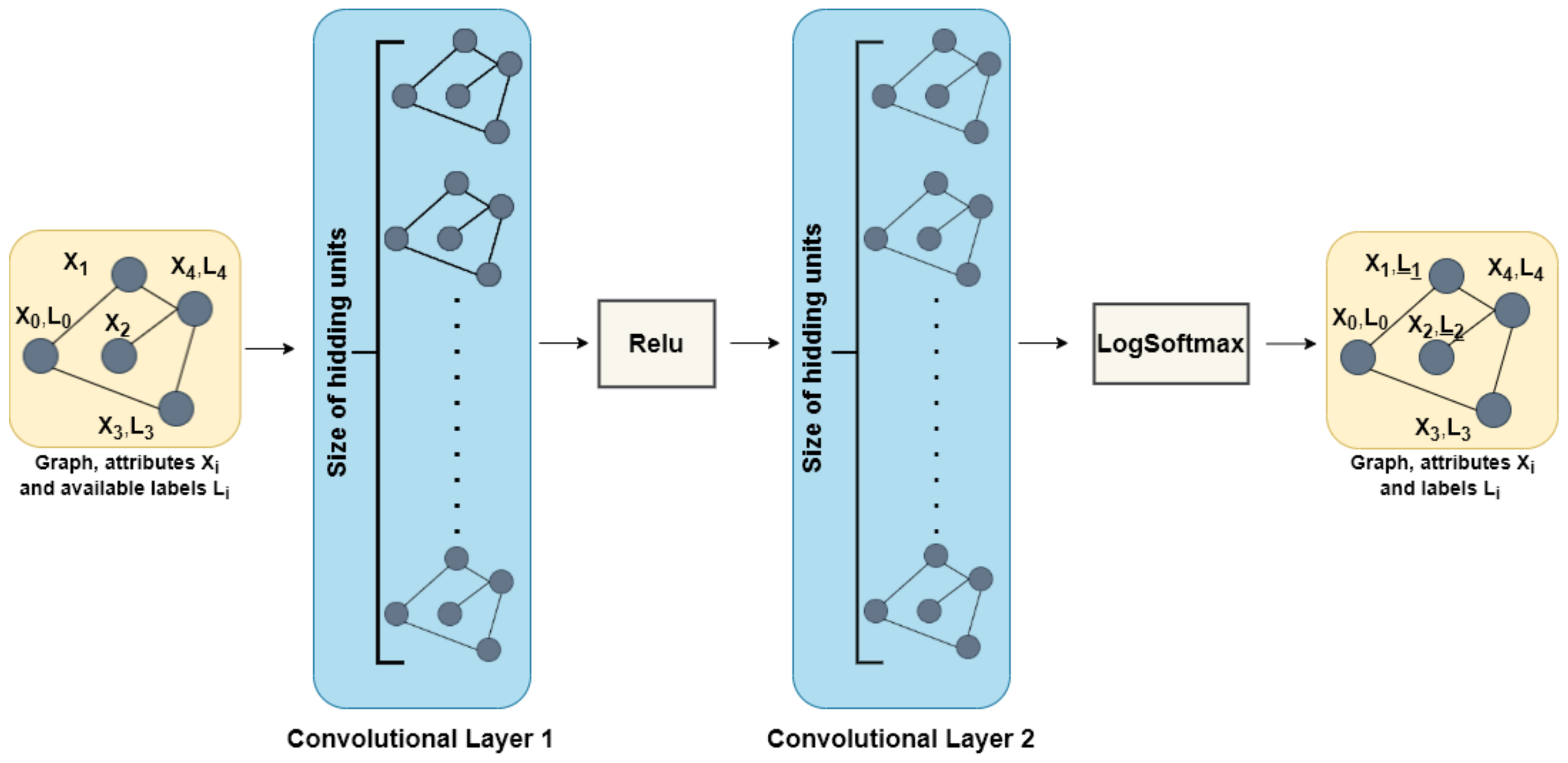
3.1. Models and Test Configurations

To highlight the added value of GCNs in this prediction task, we also apply algorithms that do not take into account topology. The GCNs’ results will thus be benchmarked against these non-topological algorithms: Support Vector Machine [51], Decision Trees [52], feedforward Artificial Neural Networks (ANN), precisely a MultiLayer Perceptron (MLP) [53], and four GCN models that have proven to be efficient in many applications. The GCN models consist of two spectral models: GCN [43] and ChebNet [46] as well as two spatial models: GraphSAGE [49] and TAGCN [50].

Given that pipe diameters and materials directly impact hydraulic modelling results, which is the aim of our work, we chose to automatically predict the missing values for each one of these two attributes. Nevertheless, other attributes could be targeted the same way.

The available attributes and their missing values are not necessarily similar and vary between providers. Hence, to investigate whether GCNs are useful in real cases, we defined two configurations based on the available data:

• Configuration 1: The network graph, a portion of the values of the targeted attribute, and domain knowledge are provided.
• Configuration 2: The network graph, a portion of the values of the targeted attribute, domain knowledge, and other fields of the attribute table are provided.

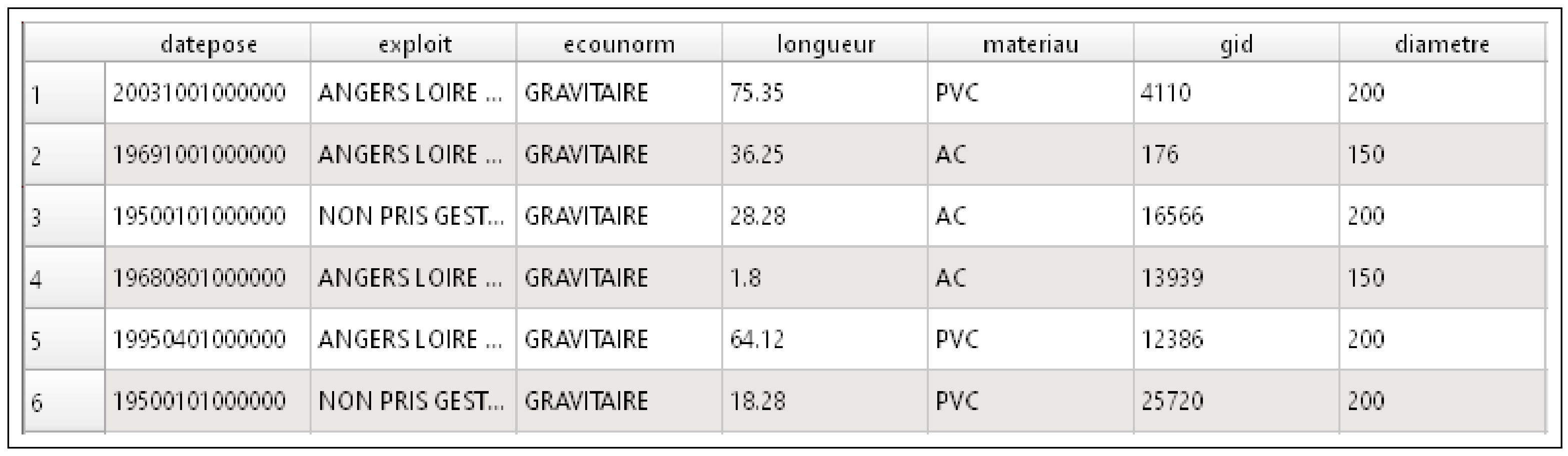
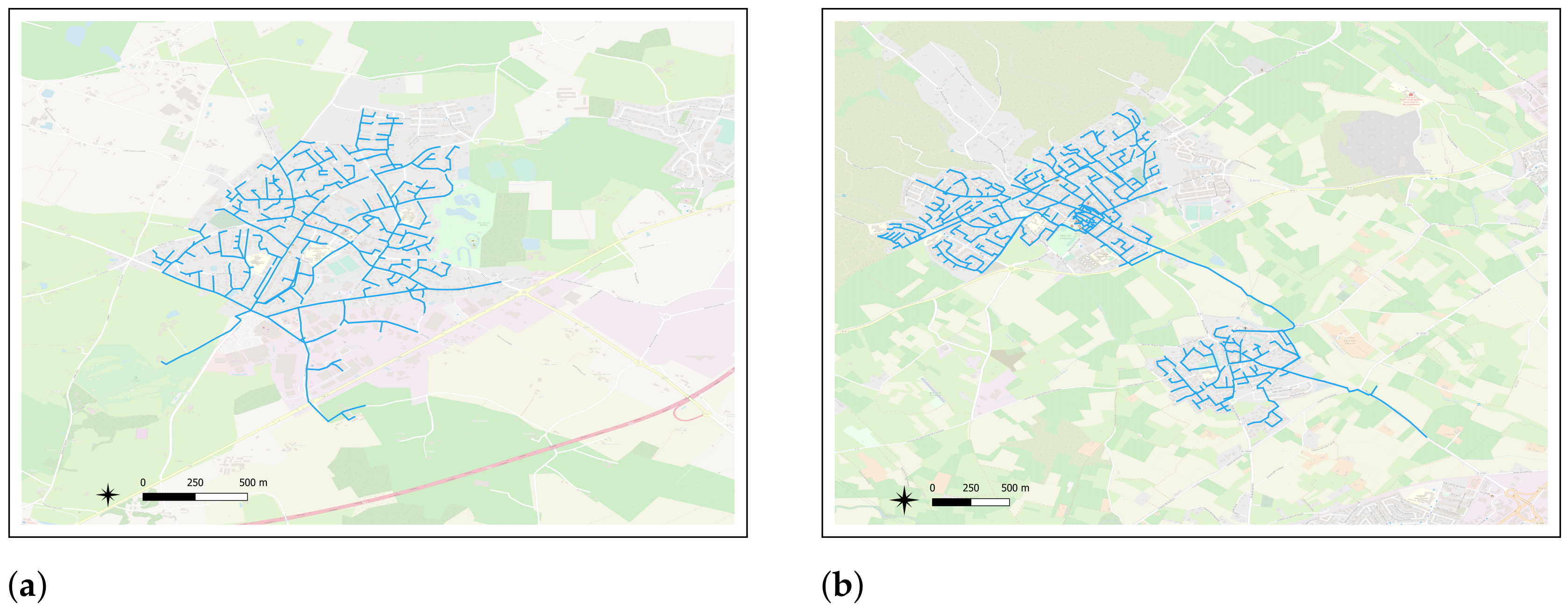
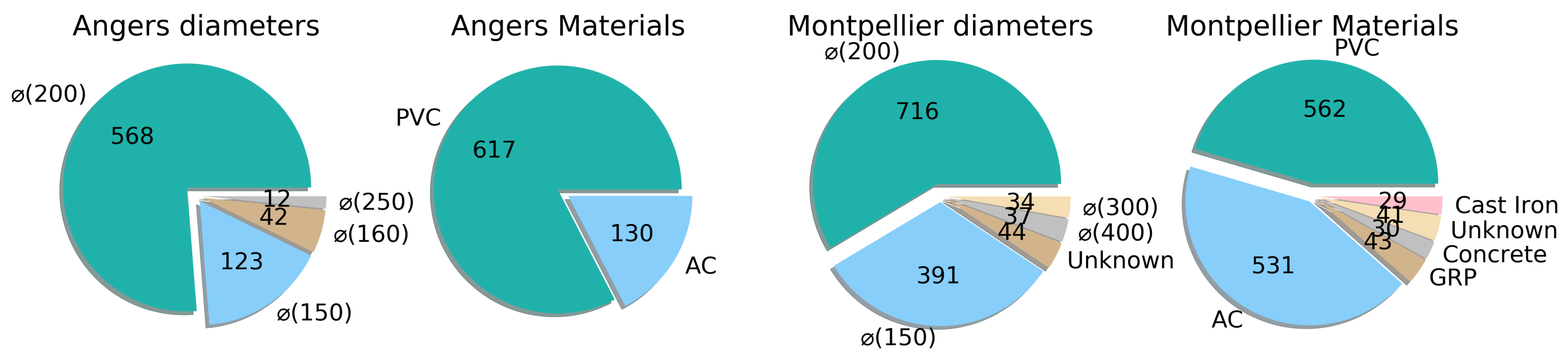
When no attributes are available, domain knowledge can be used to create and add new attributes to the structure to improve the learning process. In wastewater networks, pipe diameters increase when moving from the upstream wastewater catchments to the vicinity of the treatment plant. This domain knowledge can be accounted for using Strahler’s number, a measure of the network’s branching complexity [54]. This attribute is easily computed for each pipe since the position of treatment plants is usually known. Thus, the first configuration is conducted using the network graph and Strahler’s number as a domain knowledge attribute.

In the second configuration, managers possess more information about the networks, and relevant additional fields of the attribute table are used to infer relationships. Thus, this configuration is the richest in terms of learning material as it uses the network structure, domain knowledge, and additional characteristics to impute missing values. In this situation, the managers seek precise information about a specific attribute for various purposes, such as the diameter values for a hydraulic modelling simulation.

For each of the two configurations, the datasets were split into two subsets: Training and test. The training subset includes the available attributes of the pipes and their associated labels to be learned. However, contrary to non-topological models, in order to operate, GCN models require the structure of the graphs. Therefore, the entire structure of the graph modelled by the adjacency matrix of the wastewater network pipes was provided to this graph-based model. A total 10% of the training subset is used as a validation subset to tune the models’ parameters, that is the number of convolution layers, the number of epochs, etc.

For the MLP, we set the number of hidden layers to 3 with respectively 100, 50, and 25 units for the first, second, and third hidden layers. The number of outputs is defined by the number of classes depending on each attribute. The Rectified Linear Unit (ReLu) is used as an activation function between the layers. All layers are formed by the linear layers of PyTorch [55] and the output is computed using the Log Softmax function. For GCN models (Figure 1), we set the number of convolution layers to 2, the number of hidden units was set to 20 for the first layer, and to the number of desired classes to predict for the second layer. We used the Rectified Linear Unit (ReLu) as an activation function between the two convolutional layers, and the LogSoftmax as the activation function to output the labels. For the ChebNet layers, the filter size K was varied from 10 to 40 depending on the configuration and the size of the training subset. For the SVM model, the regularisation parameter C is set to 1 and the Radial Basis Function (RBF) is a degree 3 polynomial kernel function. For the DT models, the Splitter is set to “best”, the quality of the split is evaluated by the “Gini” criterion without any max depth constraint.

We implemented the GCN models and the MLP using PyTorch [55], where the name of the models GCN, ChebNet, GraphSAGE, and TAGCN are respectively GCNConv, ChebConv, SAGEConv, and TAGConv. The non-topological models, SVM and DT, were implemented using Scikit-learn [56].

3.2. Datasets

In this study, we used two real wastewater network databases. The first one is that of Angers Metropolis and is available through the French Government’s open access portal (https://www.data.gouv.fr/ (accessed on 1 August 2020)). The second source is the database of Montpellier Méditerranée Métropole (3M) (https://data.montpellier3m.fr/ (accessed on 1 August 2020)). These databases were chosen because they have two specific fields for the pipe diameter and material (see Figure 2 for an example of attribute tables). However, the attribute values are not all indicated and 5.9% of the total pipes of Angers and 28.63% of those of the Montpellier datasets have a missing diameter or material values.

At the scale of a metropolis, wastewater networks are usually formed of several sub-networks of cities and villages, either managed separately or linked to the main treatment plant by a unique pipe. Thus, the acquired databases are composed of several sub-graphs that represent independent wastewater networks and Strahler’s orders may be computed separately for each sub-graph. However, due to data imperfections, these disconnections may also be the result of missing spatial information such as missing pipes. Hence, to validate our results, this study was carried out on the sub-networks having the least missing attribute values. Taking into consideration possible spatial imperfections, we carefully extracted one sub-graph from each dataset (Figure 3):

• The Angers Metropolis sub-graph (Figure 3a) is composed of 754 pipes with only one unknown pipe diameter;
• The Montpellier Metropolis sub-graph (Figure 3b) is composed of 1239 pipes, with 44 pipes having unknown attribute values (either the diameter or material).

The different materials encountered in Angers metropolis are Polyvinyl Chloride (PVC), Asbestos-Cement (AC), Cast Iron, and Metal. In Montpelier metropolis we found, PVC, AC, Cast Iron, Concrete, Glass Reinforced Plastic (GRP), and Polypropylene. Ten classes of possible diameters are present in Angers’s subgraph and Montpellier’s subgraph, ranging from 80 to 500. However, for materials or diameters, several classes have less than 10 elements and will not be considered in the following. Figure 4 shows the distribution of material and diameter attributes for the considered classes, for the two data sets.

3.3. Testing Procedure

After tuning operations, the models are trained on 90% of the data and the remaining 10% are predicted. This is the first test. To put forward the models’ ability to distinguish between classes and assess their effectiveness regarding minority classes, we evaluate the results of the predictions by computing the Recall, Precision, and F1-score metrics for each class of attributes as follows:

$$\mathrm{Recall}=\frac{\mathrm{True}\mathrm{Positives}}{\mathrm{True}\mathrm{Positives}+\mathrm{False}\mathrm{Negatives}}$$

(5)

$$\mathrm{Precision}=\frac{\mathrm{True}\mathrm{Positives}}{\mathrm{True}\mathrm{Positives}+\mathrm{False}\mathrm{Positives}}$$

(6)

$$\mathrm{F}1\mathrm{Score}=2\ast \frac{\mathrm{Precision}\ast \mathrm{Recall}}{\mathrm{Precision}+\mathrm{Recall}}.$$

(7)

This prediction operation is repeated 10 times with randomly selected datasets to estimate the models’ performance more accurately. The average of these predictions is examined. To evaluate the performance of the models over each attribute, we compute the Macro-Recall, the Macro-Precision, and the Macro-F1-score as follows, where N is the number of classes of an attribute:

$$\mathrm{MacroRecall}=\frac{1}{N}\sum _i^N{\mathrm{Recall}}_i$$

(8)

$$\mathrm{MacroPrecision}=\frac{1}{N}\sum _i^N{\mathrm{Precision}}_i$$

(9)

$$\mathrm{MacroF}1\mathrm{Score}=\frac{1}{N}\sum _i^N\mathrm{F}{1}_i.$$

(10)

The training set is then sequentially reduced to increase the size of the test set, i.e., 80% for training and 20% for testing and so forth. As shown in Figure 4, attribute values are unbalanced, and the portion of the selected test subset may include only the dominant classes. Therefore, the test subset is extracted as a portion of the number of occurrences in each class. Consequently, only classes with more than 10 occurrences are considered as test subsets. For example, the diameter class of value $\varphi$(200) having 568 occurrences in the sub-graph of the Angers metropolis, the number of selected pipes for a 10% testing subset (when the task is to predict pipe diameter values) will be 56.

4. Experimental Results

In this section, we show the results of atrributes’ prediction for “Diameter” and “Material” for the two configurations described in Section 3.1. We compare the results of several experiments using the different machine learning techniques presented in the previous section. The purpose of comparing GCNs-based algorithms with different techniques of machine learning, which do not use the graph’s structure to predict missing data, is to investigate whether the network graph can facilitate missing data completion in the context of a machine learning approach. It is important to note that thanks to its structure, a GCN can predict classes without being given any attributes as input. This is clearly not possible for non-topological models. Thus, before conducting the experiments on the two defined configurations, and in order to see the behaviour of a GCN in terms of the quality of its results using only the structure of the graphs, we tested this possibility. The results show that GCN models GCNConv, SAGEConv, and TAGConv predict only the dominant classes, but the ChebConv model can identify other non-dominant classes albeit with very low recall scores such as 10% for the diameter class $\varphi$(150) on limited randomly selected test datasets. The prediction of minority classes with ChebConv, even with low scores, shows that using the structure of wastewater networks is promising.

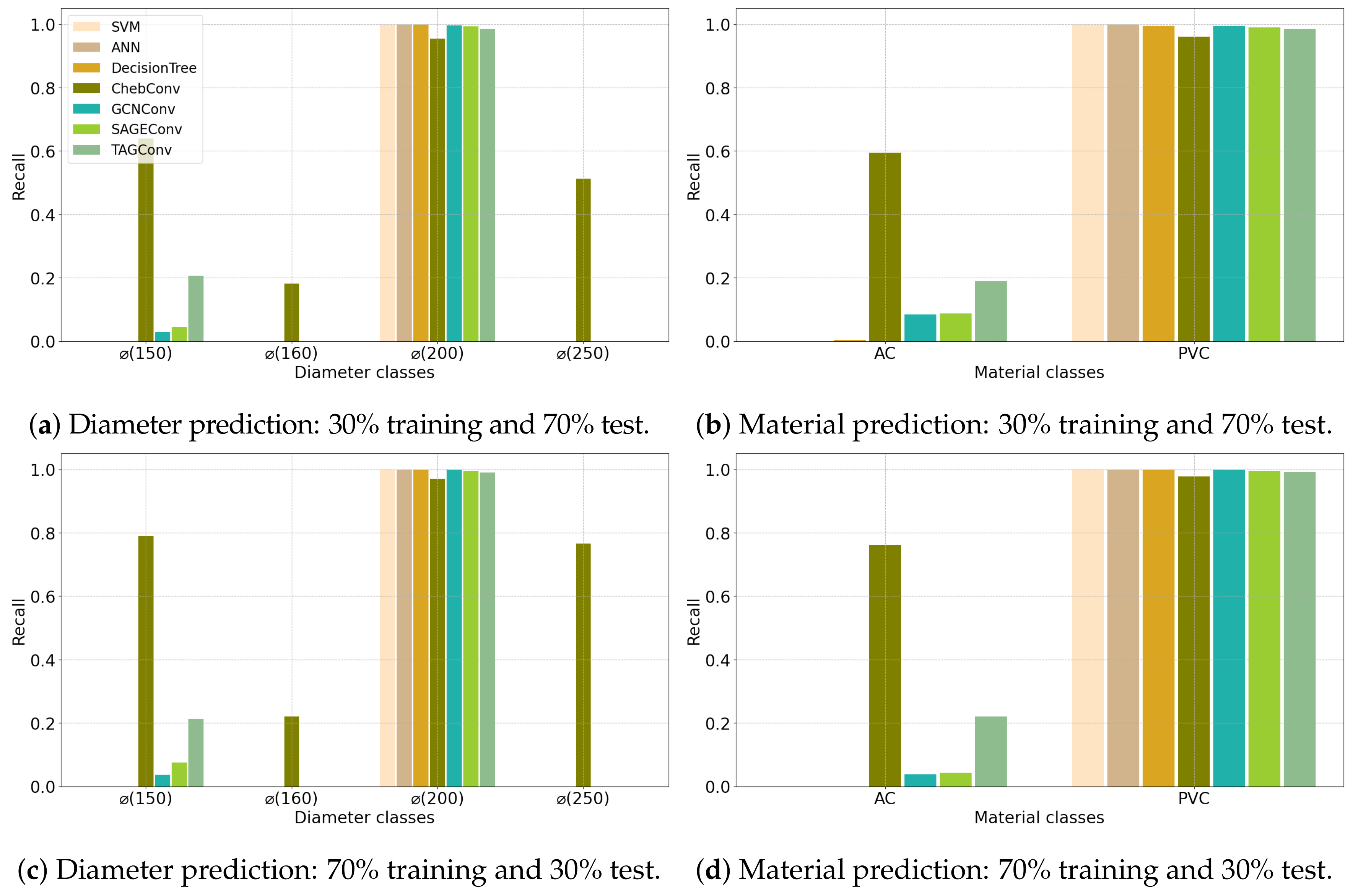
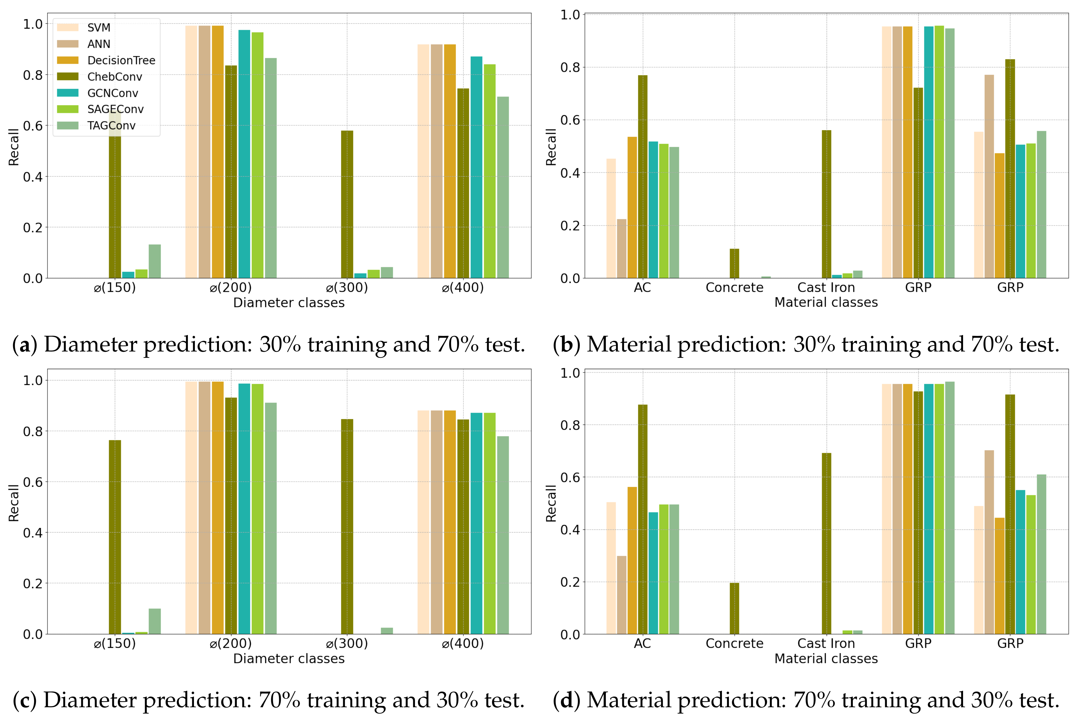
4.1. Configuration 1

In addition to the portion of the available values and the structure of the network, in this configuration, we added Strahler’s order as an attribute to help the models distinguish between the classes.

Figure 5 and Figure 6 show the results for the Angers and Montpellier datasets, respectively. Despite having difficulties with classes with small occurrences, Strahler’s order helps the models identify more classes than the dominant ones. Non-topological models SVM, Decision Tree, and MLP are unable to distinguish minor classes for the Angers dataset. Nevertheless, they predict some minor classes such as the class $\varphi$(400) with a high recall score for the Montpellier dataset (Figure 6a,c), despite having only 37 occurrences for this class. Unlike non-topological models, GCN models, namely, ChebConv and TAGConv, predict more classes for both datasets. Thus, GCN models outperform non-topological ones in terms of the number of detected classes.

ChebConv outperforms all models for both diameter and material prediction having predicted 30% of missing diameter classes $\varphi$(150) and $\varphi$(250) for the Angers dataset respectively with a recall of 79% and 77% (Figure 5c) despite having only 123 and 12 occurrences for these classes. In the case of the Montpellier dataset, ChebConv, while using only 30% of the available data, completes missing $\varphi$(150) and $\varphi$(300) diameter classes with respectively 63% and 58% recall (Figure 6a). The metric is improved when the training set is increased to 70%, thus reaching 77% and 85% respectively for these classes (Figure 6c). In comparison, the other models fail to detect these two classes for both datasets, except for TAGConv which has a very low score for the class $\varphi$(150) (Figure 5a,c and Figure 6a,c).

Similar results are obtained for material prediction. Indeed, besides having higher scores for both datasets, only GCN models predicted the AC class for Angers (Figure 5b,d). This shows that the structure of the graph and the choice of the GCN model have a great impact on the learning process.

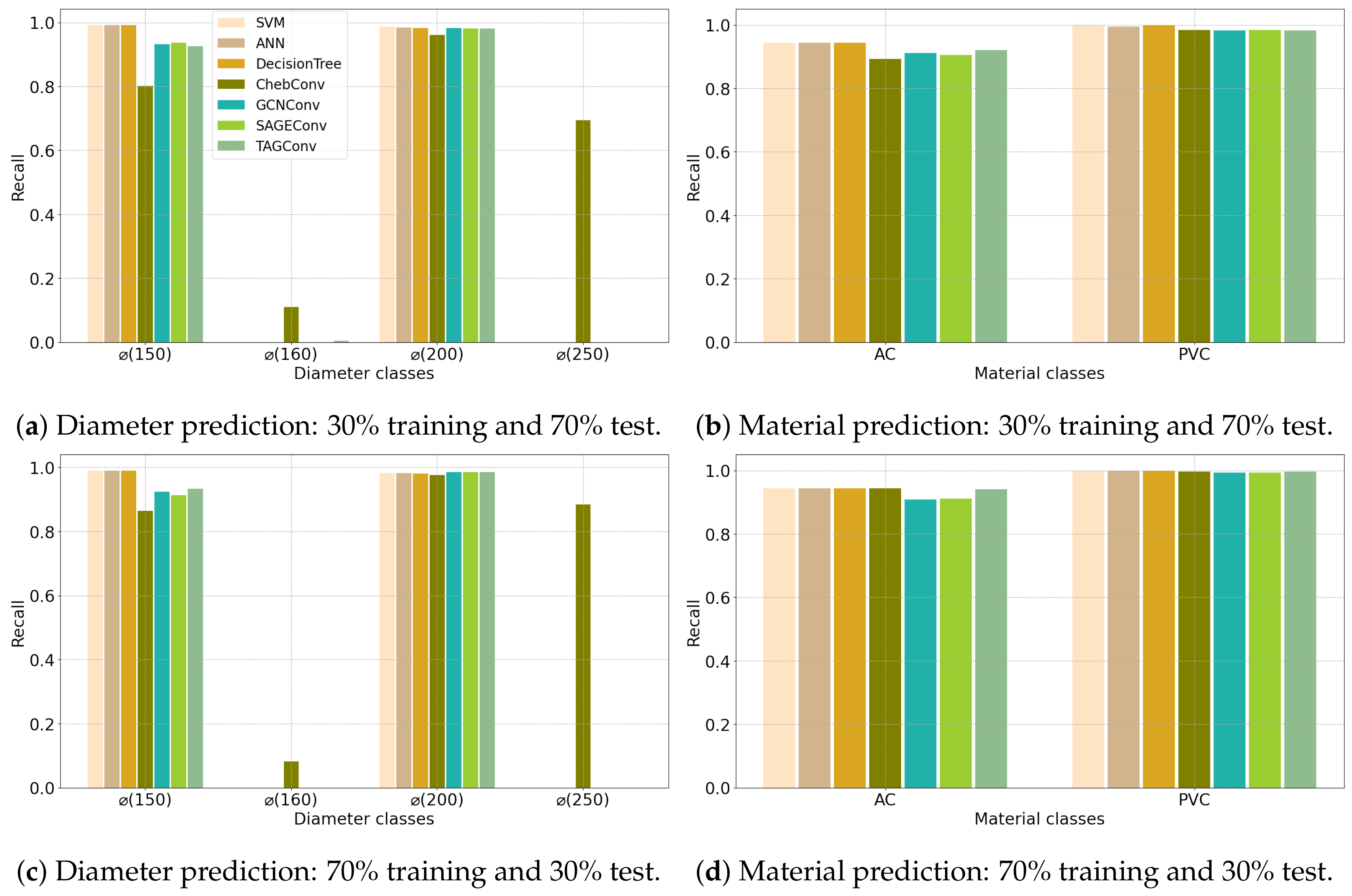
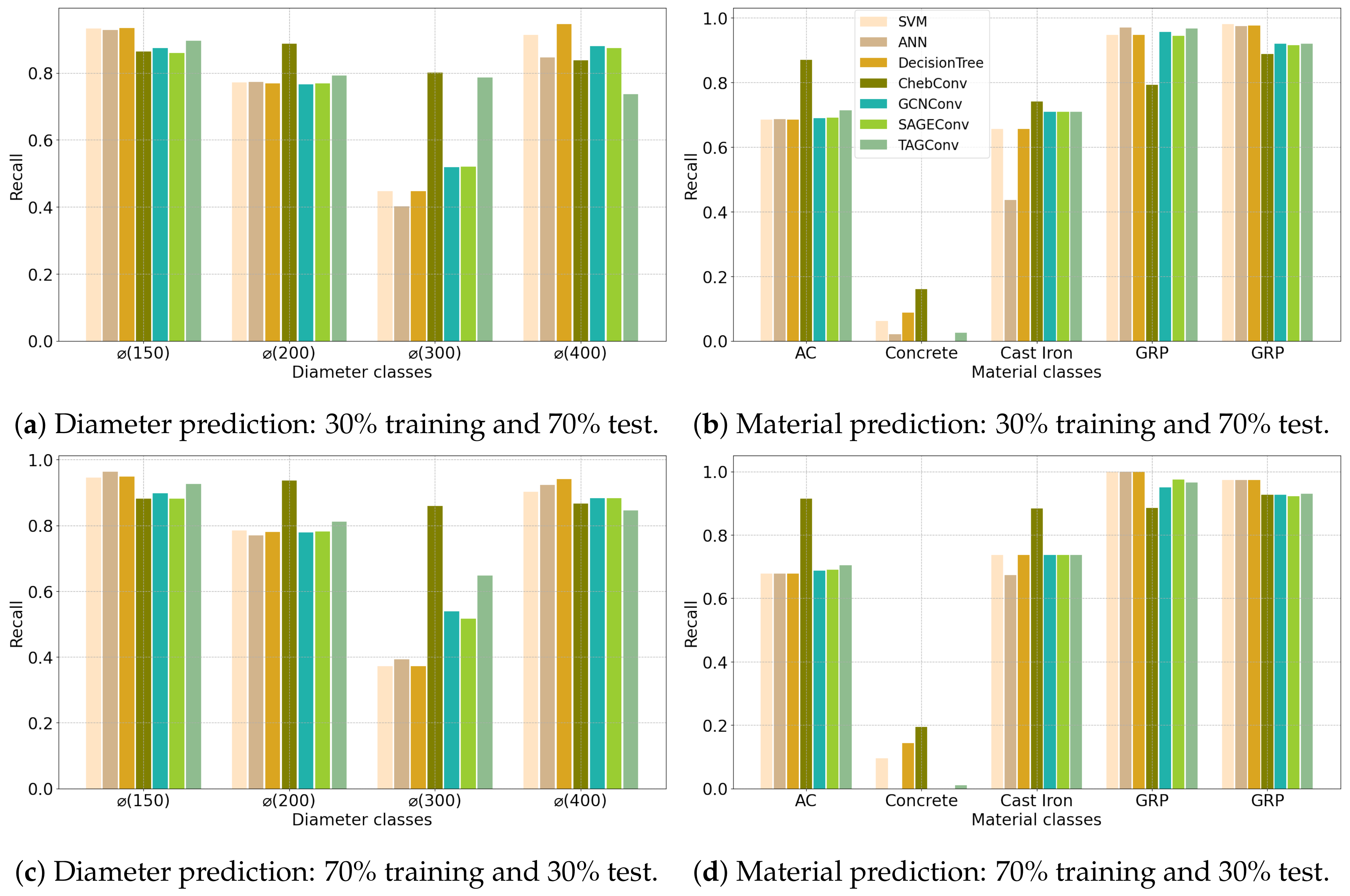
4.2. Configuration 2

In addition to the information used in the previous configuration, the attribute “material type” is added to help predict the attribute “diameter” and vice versa. The correlation between these attributes is 0.74 for the subgraph of Angers and 0.43 for the subgraph of Montpellier. Adding this information to the models substantially increases their performance regarding the number of detected classes and the recall scores. First, except for ChebConv as it already identified all the classes in the previous configuration, the number of predicted classes increases for all models. For instance, the non-topological models predict the AC class for the Angers dataset (Figure 7b). Second, Figure 7 and Figure 8, show that recall scores have increased for the majority of the classes using the various models. Still, ChebConv outperforms all models by predicting missing values with high scores for almost all classes including the minor ones, using only 30% of the available data it achieved 80% for the class $\varphi$(300), having 34 occurrences (Figure 8a) and 70% for the class $\varphi$(250), having only 12 occurrences (Figure 7a).

Table 1. Configuration 1. Results obtained for Angers and Montpellier dataset by the seven models in terms of Macro-Recall (MR), Macro-Precision (MP), and Macro-F1 (MF1) scores, for the two classes and with different percentages of the dataset used for training.

(a) Angers Dataset
		SVM			ANN			DT			ChebConv			GCNConv			SAGEConv			TAGConv
Attribute	%	MR	MP	MF1	MR	MP	MF1	MR	MP	MF1	MR	MP	MF1	MR	MP	MF1	MR	MP	MF1	MR	MP	MF1
Diameter	10	0.25	0.19	0.22	0.25	0.19	0.21	0.25	0.19	0.22	0.41	0.6	0.45	0.26	0.28	0.23	0.25	0.21	0.22	0.27	0.34	0.26
	20	0.25	0.19	0.22	0.25	0.19	0.22	0.25	0.19	0.22	0.51	0.69	0.56	0.26	0.28	0.24	0.26	0.24	0.23	0.29	0.38	0.29
	30	0.25	0.19	0.22	0.25	0.19	0.22	0.25	0.19	0.22	0.57	0.77	0.63	0.26	0.26	0.23	0.26	0.27	0.23	0.3	0.4	0.3
	40	0.25	0.19	0.22	0.25	0.19	0.22	0.25	0.19	0.22	0.61	0.79	0.66	0.26	0.26	0.23	0.26	0.26	0.23	0.3	0.42	0.3
	50	0.25	0.19	0.22	0.25	0.19	0.22	0.25	0.19	0.22	0.66	0.8	0.7	0.26	0.28	0.24	0.27	0.31	0.25	0.3	0.41	0.3
	60	0.25	0.19	0.22	0.25	0.19	0.22	0.25	0.19	0.22	0.68	0.81	0.71	0.25	0.23	0.23	0.27	0.36	0.26	0.3	0.41	0.31
	70	0.25	0.19	0.22	0.25	0.19	0.22	0.25	0.19	0.22	0.69	0.77	0.71	0.26	0.29	0.23	0.27	0.35	0.25	0.3	0.4	0.3
	80	0.25	0.19	0.22	0.25	0.19	0.22	0.25	0.19	0.22	0.69	0.78	0.72	0.26	0.28	0.23	0.26	0.29	0.24	0.3	0.41	0.3
	90	0.25	0.19	0.22	0.25	0.19	0.22	0.25	0.19	0.22	0.75	0.76	0.74	0.27	0.29	0.24	0.26	0.27	0.23	0.31	0.43	0.31
Material	10	0.5	0.42	0.45	0.5	0.41	0.45	0.49	0.43	0.45	0.62	0.78	0.66	0.54	0.69	0.53	0.52	0.63	0.5	0.56	0.73	0.57
	20	0.5	0.41	0.45	0.5	0.41	0.45	0.5	0.41	0.45	0.71	0.82	0.75	0.53	0.66	0.51	0.53	0.6	0.5	0.59	0.83	0.61
	30	0.5	0.41	0.45	0.5	0.41	0.45	0.5	0.42	0.45	0.78	0.86	0.81	0.54	0.74	0.53	0.54	0.71	0.53	0.59	0.81	0.6
	40	0.5	0.41	0.45	0.5	0.41	0.45	0.5	0.41	0.45	0.85	0.89	0.86	0.54	0.76	0.53	0.54	0.74	0.53	0.6	0.82	0.63
	50	0.5	0.41	0.45	0.5	0.41	0.45	0.5	0.41	0.45	0.86	0.88	0.87	0.54	0.76	0.53	0.55	0.77	0.54	0.6	0.87	0.63
	60	0.5	0.41	0.45	0.5	0.41	0.45	0.5	0.41	0.45	0.87	0.9	0.89	0.53	0.64	0.5	0.54	0.73	0.53	0.6	0.83	0.63
	70	0.5	0.41	0.45	0.5	0.41	0.45	0.5	0.41	0.45	0.87	0.92	0.89	0.52	0.6	0.49	0.52	0.61	0.49	0.61	0.85	0.63
	80	0.5	0.42	0.45	0.5	0.42	0.45	0.5	0.42	0.45	0.88	0.93	0.9	0.53	0.75	0.52	0.53	0.75	0.52	0.6	0.87	0.63
	90	0.5	0.41	0.45	0.5	0.41	0.45	0.5	0.41	0.45	0.91	0.95	0.93	0.53	0.64	0.5	0.53	0.64	0.5	0.62	0.91	0.65
(b) Montpellier Dataset
		SVM			ANN			DT			ChebConv			GCNConv			SAGEConv			TAGConv
Attribute	%	MR	MP	MF1	MR	MP	MF1	MR	MP	MF1	MR	MP	MF1	MR	MP	MF1	MR	MP	MF1	MR	MP	MF1
Diameter	10	0.22	0.16	0.18	0.23	0.16	0.19	0.22	0.17	0.19	0.48	0.62	0.52	0.23	0.38	0.23	0.23	0.37	0.23	0.38	0.52	0.41
	20	0.25	0.17	0.2	0.36	0.24	0.29	0.38	0.26	0.31	0.63	0.74	0.67	0.39	0.44	0.37	0.39	0.47	0.37	0.43	0.5	0.43
	30	0.48	0.31	0.38	0.48	0.31	0.38	0.48	0.31	0.38	0.7	0.78	0.73	0.47	0.39	0.39	0.47	0.43	0.4	0.44	0.47	0.42
	40	0.48	0.32	0.38	0.48	0.32	0.38	0.48	0.32	0.38	0.76	0.85	0.79	0.46	0.37	0.39	0.46	0.37	0.39	0.44	0.52	0.42
	50	0.48	0.31	0.38	0.48	0.31	0.38	0.48	0.31	0.38	0.8	0.88	0.83	0.47	0.34	0.39	0.47	0.35	0.39	0.47	0.53	0.43
	60	0.48	0.32	0.38	0.48	0.32	0.38	0.48	0.32	0.38	0.83	0.88	0.84	0.48	0.33	0.39	0.48	0.35	0.39	0.46	0.53	0.42
	70	0.47	0.32	0.38	0.47	0.32	0.38	0.47	0.32	0.38	0.85	0.91	0.87	0.47	0.34	0.38	0.47	0.34	0.38	0.45	0.46	0.41
	80	0.49	0.34	0.4	0.49	0.34	0.4	0.49	0.34	0.4	0.85	0.91	0.87	0.48	0.34	0.4	0.48	0.35	0.4	0.48	0.55	0.44
	90	0.47	0.33	0.38	0.47	0.33	0.38	0.47	0.33	0.38	0.87	0.91	0.88	0.47	0.33	0.38	0.47	0.33	0.38	0.46	0.5	0.41
Material	10	0.36	0.33	0.33	0.35	0.29	0.31	0.36	0.33	0.32	0.43	0.55	0.45	0.36	0.33	0.34	0.36	0.33	0.33	0.35	0.36	0.34
	20	0.39	0.33	0.34	0.39	0.31	0.33	0.39	0.32	0.34	0.55	0.68	0.57	0.39	0.35	0.35	0.4	0.36	0.36	0.39	0.37	0.36
	30	0.39	0.32	0.35	0.39	0.28	0.32	0.39	0.33	0.35	0.6	0.69	0.62	0.4	0.37	0.36	0.4	0.35	0.36	0.41	0.39	0.37
	40	0.39	0.33	0.35	0.39	0.31	0.33	0.39	0.33	0.35	0.64	0.75	0.65	0.39	0.33	0.35	0.39	0.34	0.35	0.41	0.38	0.38
	50	0.39	0.32	0.34	0.39	0.27	0.31	0.39	0.33	0.34	0.68	0.84	0.71	0.39	0.33	0.35	0.39	0.33	0.34	0.42	0.4	0.38
	60	0.39	0.33	0.34	0.39	0.3	0.32	0.39	0.33	0.34	0.72	0.85	0.76	0.39	0.33	0.35	0.39	0.34	0.35	0.42	0.38	0.38
	70	0.39	0.32	0.34	0.39	0.3	0.33	0.39	0.32	0.34	0.72	0.83	0.75	0.39	0.33	0.35	0.4	0.35	0.35	0.42	0.36	0.38
	80	0.38	0.33	0.33	0.38	0.29	0.32	0.38	0.33	0.33	0.72	0.88	0.75	0.37	0.31	0.33	0.38	0.32	0.34	0.41	0.36	0.37
	90	0.39	0.33	0.33	0.38	0.28	0.31	0.39	0.34	0.32	0.74	0.78	0.75	0.4	0.35	0.36	0.39	0.33	0.34	0.44	0.4	0.41

and

Table 2. Configuration 2. Results obtained for Angers and Montpellier dataset by the seven models in terms of Macro-Recall (MR), Macro-Precision (MP), and Macro-F1 (MF1) scores, for the two classes and with different percentages of the dataset used for training.

(a) Angers Dataset
		SVM			ANN			DT			ChebConv			GCNConv			SAGEConv			TAGConv
Attribute	%	MR	MP	MF1	MR	MP	MF1	MR	MP	MF1	MR	MP	MF1	MR	MP	MF1	MR	MP	MF1	MR	MP	MF1
Diameter	10	0.49	0.46	0.47	0.49	0.46	0.48	0.49	0.46	0.48	0.58	0.76	0.62	0.48	0.45	0.46	0.47	0.45	0.46	0.48	0.5	0.47
	20	0.49	0.46	0.48	0.49	0.46	0.48	0.49	0.46	0.48	0.64	0.74	0.66	0.48	0.45	0.46	0.48	0.45	0.46	0.48	0.46	0.47
	30	0.49	0.46	0.48	0.49	0.46	0.48	0.49	0.46	0.48	0.64	0.73	0.66	0.48	0.45	0.47	0.48	0.45	0.47	0.48	0.46	0.47
	40	0.49	0.46	0.48	0.49	0.46	0.47	0.49	0.46	0.47	0.68	0.76	0.7	0.48	0.45	0.47	0.48	0.45	0.47	0.49	0.46	0.47
	50	0.49	0.46	0.48	0.49	0.46	0.48	0.49	0.46	0.48	0.67	0.79	0.69	0.48	0.45	0.47	0.48	0.45	0.47	0.48	0.46	0.47
	60	0.49	0.46	0.48	0.49	0.46	0.48	0.49	0.46	0.48	0.68	0.8	0.7	0.48	0.45	0.47	0.48	0.45	0.47	0.48	0.46	0.47
	70	0.49	0.46	0.48	0.49	0.46	0.47	0.49	0.46	0.48	0.7	0.77	0.71	0.48	0.46	0.47	0.47	0.46	0.47	0.48	0.46	0.47
	80	0.5	0.46	0.48	0.5	0.46	0.48	0.5	0.46	0.48	0.66	0.71	0.66	0.48	0.45	0.46	0.48	0.45	0.46	0.48	0.46	0.47
	90	0.49	0.46	0.48	0.49	0.46	0.48	0.49	0.46	0.48	0.74	0.77	0.74	0.48	0.45	0.47	0.48	0.46	0.47	0.48	0.46	0.47
Material	10	0.96	0.99	0.97	0.96	0.99	0.97	0.97	0.99	0.98	0.87	0.93	0.9	0.93	0.95	0.94	0.92	0.95	0.94	0.9	0.94	0.92
	20	0.96	0.99	0.98	0.97	0.99	0.98	0.97	0.99	0.98	0.91	0.94	0.92	0.94	0.96	0.95	0.94	0.95	0.95	0.94	0.96	0.95
	30	0.97	0.99	0.98	0.97	0.99	0.98	0.97	0.99	0.98	0.94	0.96	0.95	0.95	0.95	0.95	0.94	0.96	0.95	0.95	0.96	0.96
	40	0.97	0.99	0.98	0.97	0.99	0.98	0.97	0.99	0.98	0.94	0.96	0.95	0.94	0.96	0.95	0.94	0.95	0.95	0.95	0.96	0.96
	50	0.97	0.99	0.98	0.97	0.99	0.98	0.97	0.99	0.98	0.95	0.97	0.96	0.95	0.96	0.95	0.94	0.96	0.95	0.96	0.98	0.97
	60	0.98	0.99	0.98	0.98	0.99	0.98	0.98	0.99	0.98	0.97	0.97	0.97	0.96	0.97	0.96	0.96	0.97	0.96	0.97	0.98	0.97
	70	0.97	0.99	0.98	0.97	0.99	0.98	0.97	0.99	0.98	0.97	0.99	0.98	0.95	0.97	0.96	0.95	0.97	0.96	0.97	0.99	0.98
	80	0.96	0.99	0.98	0.96	0.99	0.98	0.96	0.99	0.98	0.95	0.98	0.96	0.94	0.96	0.95	0.94	0.96	0.95	0.96	0.98	0.97
	90	0.95	0.99	0.97	0.95	0.99	0.97	0.95	0.99	0.97	0.97	0.97	0.97	0.93	0.96	0.94	0.93	0.96	0.94	0.95	0.99	0.97
(b) Montpellier Dataset
		SVM			ANN			DT			ChebConv			GCNConv			SAGEConv			TAGConv
Attribute	%	MR	MP	MF1	MR	MP	MF1	MR	MP	MF1	MR	MP	MF1	MR	MP	MF1	MR	MP	MF1	MR	MP	MF1
Diameter	10	0.5	0.64	0.52	0.51	0.58	0.52	0.51	0.6	0.52	0.75	0.86	0.79	0.52	0.64	0.54	0.52	0.61	0.54	0.67	0.83	0.73
	20	0.54	0.64	0.55	0.64	0.69	0.64	0.59	0.68	0.6	0.82	0.89	0.85	0.7	0.81	0.72	0.68	0.82	0.71	0.77	0.84	0.79
	30	0.77	0.86	0.79	0.74	0.81	0.75	0.77	0.85	0.79	0.85	0.9	0.87	0.76	0.85	0.79	0.76	0.84	0.79	0.8	0.86	0.82
	40	0.77	0.85	0.77	0.77	0.81	0.75	0.78	0.84	0.77	0.88	0.92	0.9	0.79	0.83	0.79	0.78	0.82	0.78	0.81	0.85	0.82
	50	0.77	0.86	0.79	0.78	0.85	0.79	0.79	0.85	0.79	0.88	0.92	0.9	0.79	0.83	0.8	0.79	0.84	0.8	0.81	0.88	0.83
	60	0.8	0.86	0.81	0.77	0.83	0.78	0.8	0.85	0.81	0.9	0.93	0.91	0.82	0.83	0.82	0.82	0.83	0.81	0.85	0.86	0.85
	70	0.75	0.85	0.77	0.76	0.84	0.77	0.76	0.85	0.77	0.89	0.93	0.91	0.77	0.82	0.79	0.77	0.82	0.78	0.81	0.86	0.82
	80	0.75	0.81	0.76	0.77	0.86	0.78	0.75	0.81	0.76	0.89	0.93	0.91	0.79	0.82	0.79	0.79	0.82	0.79	0.85	0.87	0.85
	90	0.79	0.81	0.78	0.79	0.8	0.78	0.79	0.8	0.78	0.89	0.96	0.91	0.84	0.85	0.83	0.84	0.83	0.83	0.9	0.87	0.88
Material	10	0.6	0.72	0.63	0.54	0.52	0.52	0.6	0.68	0.61	0.54	0.73	0.57	0.6	0.65	0.61	0.6	0.64	0.61	0.63	0.7	0.65
	20	0.66	0.73	0.68	0.63	0.65	0.63	0.66	0.76	0.68	0.65	0.78	0.68	0.64	0.68	0.65	0.63	0.68	0.64	0.65	0.71	0.66
	30	0.67	0.79	0.7	0.62	0.71	0.64	0.67	0.81	0.7	0.69	0.81	0.72	0.65	0.7	0.67	0.65	0.69	0.66	0.67	0.73	0.68
	40	0.67	0.77	0.7	0.64	0.7	0.66	0.68	0.82	0.72	0.71	0.82	0.74	0.65	0.69	0.66	0.64	0.68	0.65	0.66	0.72	0.68
	50	0.68	0.76	0.7	0.65	0.7	0.66	0.7	0.83	0.73	0.73	0.85	0.76	0.67	0.7	0.67	0.65	0.67	0.65	0.67	0.71	0.68
	60	0.69	0.81	0.72	0.67	0.72	0.68	0.69	0.84	0.72	0.72	0.81	0.74	0.64	0.69	0.65	0.65	0.69	0.66	0.66	0.71	0.67
	70	0.7	0.83	0.72	0.66	0.7	0.67	0.71	0.87	0.74	0.76	0.81	0.77	0.66	0.7	0.67	0.66	0.69	0.67	0.67	0.72	0.68
	80	0.67	0.78	0.7	0.65	0.71	0.66	0.68	0.82	0.71	0.73	0.84	0.76	0.65	0.69	0.66	0.65	0.69	0.66	0.66	0.72	0.67
	90	0.72	0.78	0.73	0.65	0.69	0.66	0.72	0.78	0.73	0.79	0.8	0.79	0.68	0.69	0.67	0.68	0.67	0.66	0.68	0.7	0.68

display the scores, Macro-Recall (MR), Macro-Precision (MP), and Macro-F1 Score (MF1) for each attribute of the two datasets of Angers and Montpellier for configurations 1 and 2 respectively, and the nine different percentages of the dataset used for training. First, for configuration 1, for both cities, Table 1a,b show, as indicated before, a poor performance of the non-topological models. This has been expected since they use only Strahler’s order to distinguish the different classes, while graph models use the adjacency matrix. As for configuration 2, the scores increase for all models. Thus, the performance of non-topological models relies only on the correlations (

Table 3. Attributes correlations.

Angers Dataset
Attributes	Diameter	Material	Strahler
Diameter	1	0.74	0.06
Material	0.74	1	0.01
Strahler	0.06	0.01	1
Montpellier Dataset
Attributes	Diameter	Material	Strahler
Diameter	1	0.43	0.31
Material	0.43	1	0.08
Strahler	0.31	0.08	1

) between Strahler’s order and the targeted attributes. Second, except for ChebConv, whose performance increases when the portion of missing values decreases, all the models’ performances are generally constant in configuration 1 for the Angers dataset (Table 1a) since they predict only the dominant classes. This is also to be expected for non-topological models, since there is no correlation between Strahler’s order and both attributes, diameter, and material, for this dataset. However, for the Montpellier dataset, (Table 1b) where the correlation between material and Strahler is 0.08 and between the diameter and Strahler the correlation is 0.31, the non-topological models’ performances increase when the percentage of missing data decreases for the attribute diameter. In addition, in configuration 2, the models’ performances evolve differently for the two datasets. For Angers, all models are nearly constant, although a small increase can be noted in ChebConv’s performance while the missing data decreases. These scores (Table 2a) can be explained by the high correlation of the attributes material and diameter (0.74). For the Montpellier dataset, where the correlation is lower compared to the Angers dataset, almost all the models’ performances increase. Figure 9 illustrates this evolution using the Macro-F1Score metric. The differences in performance related to the GCN models are detailed in the next paragraph.

Our experiments show that for real-world configurations, ChebConv yields the best results for both datasets and both predicted attributes. Spatial approaches fail to distinguish minority classes compared to the spectral approaches (i.e., ChebConv) and slightly outperform non-topological approaches. The fact that SAGEConv, which is a spatial approach, has a nearly similar evolution performance as non-topological models, and is outperformed by ChebConv, may be explained by the fixed-size set of the neighbourhood, where not all the neighbourhoods are explored. Furthermore, for the spectral approaches, ChebConv surpassing GCNConv may be explained by the differences in the number of K-localised filters since GCNConv uses only $K=1$ to avoid overfitting. To confirm this assumption we varied the values of parameter K to 1, 10, 15, and 20 for the ChebConv model and compared the new experiments to the GCNConv. Figure 10 shows that GCNConv and ChebConv with $K=1$ have similar performances regarding the number of predicted classes and the recall scores, when predicting the diameter values for the Montpellier dataset. Moreover, comparing the performance of ChebConv with different K values shows that increasing the number of neighbour nodes used in the learning process improves the prediction results. This was also noted for TAGConv.

5. Discussion and Conclusions

This study was conducted to investigate whether machine learning algorithms can be used for Missing Value Imputation on wastewater networks. We carried out tests using seven different models; four Graph Convolutional Network models: GCN, ChebNet, TAGCN, and GraphSAGE, and three popular non-topological models: SVM, Decision Trees, and a MultiLayer Perceptron. The results show that machine learning models are an efficient tool for completing missing attributes for wastewater networks when various types of information about a network are available. This is highlighted in the second test configuration we explored. Moreover, for extreme situations, when only the network layout and partial attribute information are available (i.e., the first test configuration), the ChebConv spectral GCN approach, which is based on the approximation of the spectrum of the graph Laplacian, yields the best results for the completion of attribute values in general, and minority classes in particular. ChebConv also yields acceptable results when a small percentage of the available data is used for training. This was demonstrated in several studies using GCN-based models. The work of [32] demonstrated that, in comparison with other approaches such as KNN, the performance of their GCN-based model increases substantially when the percentage of the missing data increases. In a different application, similar conclusions were reached by [57] when inferring users’ geo-localisation in social media. The authors used a semi-supervised configuration combining graph structure and text and showed that a GCN-based model performs well in scenarios with minimal supervision by effectively using unlabelled data.

The machine learning models that we used in this application require specific conditions. First, the classes to be learnt must be part of the training dataset. We complied with this request by ignoring classes with less than 10 occurrences. However, this led to fewer minority classes in the test subset and therefore impacted the prediction results substantially. Second, machine learning models are known to require important data quantity to achieve satisfying results. Having achieved these scores while using such restricted datasets shows that this approach can be even more promising with larger datasets. We would like also to emphasise that our objective was not to determine the best GCN architecture for wastewater network data completion, but rather to investigate the impact of the structure of the graph as a learning factor on the prediction results. In this study, we used the default implementation of the GCN models as described in the original papers. Although these models showed excellent performance in various domains such as information science, bibliometrics, water distribution systems, or biology [43,49,50,58], they can be further adapted to the specific context of each domain to produce better results. For instance, in [59], a novel type of GCN for road networks called Relational Fusion Network (RFN) is put forward for driving speed estimation and speed limit classification. The results indicate that RFN outperforms state-of-the-art GCN algorithms such as GraphSAGE in this application.

To assess whether the structure of the graph, modelled in our case by the adjacency matrix, has an impact on the learning process, non-topological models were trained using only the available attributes. That is Strahler’s order for the first configuration and Strahler’s order, diameter, and material for the second configuration. Strahler’s order is used as a proxy for network topology in these models. For the GCN models, in addition to these attributes, the adjacency matrix is required and is also provided. The matrix is not used for the non-topological models because they are not built to deal with graph structures and require a pre-processing step to operate. This consists in representing or encoding the graph in a suitable form for the targeted model. As stated in Section 2, this operation is complex and does not guarantee the full use of the graph structure, while GCN models can easily handle information such as adjacency or angle between pipes to perform MVI operations. Therefore, no pre-processing was carried out in this work.

The attributes diameter, material, and Strahler’s order were used only as illustration examples in this study. We aim to show that machine learning models can be an efficient method to help all entities facing the problem of missing wastewater network data, to overcome this challenge. The use of both numerical (diameter) and categorical (material) attributes shows that this approach overcomes the limits of the statistical methods used in [18]. In some instances, Strahler’s order, which is dependent on the dataset, may not be the best descriptor. For instance, since the Angers dataset is very small, the pipe diameters do not increase when moving from the upstream wastewater catchments to the vicinity of the treatment plant. This leads to a lack of correlation between Strahler’s order and diameter (Table 3). Thus, Strahler’s order does not affect the diameter predictions for the Angers dataset, contrary to the Montpellier network. One may also use the type of buildings near the pipes as an attribute to predict their diameter. The main idea is that, since network construction rules vary from one country to another, and between regions of the same country, machine learning models can easily integrate new information to make predictions and improve them. It all depends on the available data and knowledge about the targeted network.

Urban managers and environmental monitoring services are often faced with incomplete data sets and have to resort to Missing Value Imputation (MVI) or Missing Data Imputation (MDI) algorithms. GCN models would provide managers with an additional accessible resource to overcome data imperfection challenges and support decision makers, be it to conduct repairs, predict future damages such as in [60], or run a hydraulic simulation model. Indeed, several urban utility networks such as gas, water, and electrical supplies are structured as graphs with nodes and edges. Our proposition would help asset management tasks by providing a better estimate for given characteristics of the undocumented portions of the network. Another important feature of Smart City management plans is air and water pollution monitoring. Given the spatial and temporal variability of environmental indicators, these monitoring plans rely on a network of sensors, spread out over large geographical areas. As with any piece of equipment, these devices are prone to failure and damage, resulting in missing data. By resorting to GNNs, managers would be able to extract the most of their network’s structure and gain more accurate estimations of the missing data. They would thus be able to better inform citizens and improve their quality of life.

References

1. UN. Population Division of the Department of Economic and Social Affairs of the United Nations: World Urbanization Prospects: The 2018 Revision; Technical Report (ST/ESA/SER.A/420); UN: New York, NY, USA, 2019. [Google Scholar]
2. OECD. OECD Environmental Outlook to 2050: The Consequences of Inaction; OECD Editions: Paris, France, 2012; p. 350. [Google Scholar] [CrossRef]
3. Yuan, Z.; Olsson, G.; Cardell-Oliver, R.; van Schagen, K.; Marchi, A.; Deletic, A.; Urich, C.; Rauch, W.; Liu, Y.; Jiang, G. Sweating the assets—The role of instrumentation, control and automation in urban water systems. Water Res. 2019, 155, 381–402. [Google Scholar] [CrossRef]
4. Harrison, C.; Eckman, B.; Hamilton, R.; Hartswick, P.; Kalagnanam, J.; Paraszczak, J.; Williams, P. Foundations for Smarter Cities. IBM J. Res. Dev. 2010, 54, 1–16. [Google Scholar] [CrossRef]
5. Nie, X.; Fan, T.; Wang, B.; Li, Z.; Shankar, A.; Manickam, A. Big Data analytics and IoT in Operation safety management in Under Water Management. Comput. Commun. 2020, 154, 188–196. [Google Scholar] [CrossRef]
6. Chen, Y.; Han, D. Water quality monitoring in smart city: A pilot project. Autom. Constr. 2018, 89, 307–316. [Google Scholar] [CrossRef] [Green Version]
7. Kofinas, D.T.; Spyropoulou, A.; Laspidou, C.S. A methodology for synthetic household water consumption data generation. Environ. Model. Softw. 2018, 100, 48–66. [Google Scholar] [CrossRef]
8. Zeng, Z.; Yuan, X.; Liang, J.; Li, Y. Designing and implementing an SWMM-based web service framework to provide decision support for real-time urban stormwater management. Environ. Model. Softw. 2021, 135, 104887. [Google Scholar] [CrossRef]
9. Gibert, K.; Sànchez-Marrè, M.; Rodríguez-Roda, I. GESCONDA: An intelligent data analysis system for knowledge discovery and management in environmental databases. Environ. Model. Softw. 2006, 21, 115–120. [Google Scholar] [CrossRef]
10. Lin, P.; Yuan, X.X. A two-time-scale point process model of water main breaks for infrastructure asset management. Water Res. 2019, 150, 296–309. [Google Scholar] [CrossRef]
11. Junninen, H.; Niska, H.; Tuppurainen, K.; Ruuskanen, J.; Kolehmainen, M. Methods for imputation of missing values in air quality data sets. Atmos. Environ. 2004, 38, 2895–2907. [Google Scholar] [CrossRef]
12. Schneider, T. Analysis of incomplete climate data: Estimation of Mean Values and covariance matrices and imputation of Missing values. J. Clim. 2001, 14, 853–871. [Google Scholar] [CrossRef]
13. ASTEE. Gestion Patrimoniale des Réseaux D’assainissement; ASTEE: Nanterre, France, 2015. [Google Scholar]
14. Chen, H.; Cohn, A.G. Buried utility pipeline mapping based on multiple spatial data sources: A Bayesian data fusion approach. In Twenty-Second International Joint Conference on Artificial Intelligence; IJCAI: Barcelona, Catalonia, Spain, 2011; pp. 2411–2417. ISBN 978-1-57735-516-8. [Google Scholar]
15. Bilal, M.; Khan, W.; Muggleton, J.; Rustighi, E.; Jenks, H.; Pennock, S.R.; Atkins, P.R.; Cohn, A. Inferring the most probable maps of underground utilities using Bayesian mapping model. J. Appl. Geophys. 2018, 150, 52–66. [Google Scholar] [CrossRef]
16. Hafsi, M.; Bolon, P.; Dapoigny, R. Detection and localization of underground networks by fusion of electromagnetic signal and GPR images. In Proceedings SPIE 10338, Thirteenth International Conference on Quality Control by Artificial Vision 2017, Tokyo, Japan; Nagahara, H., Umeda, K., Yamashita, A., Eds.; International Society for Optics and Photonics: Bellingham, WA, USA, 2017; Volume 10338, pp. 7–14. [Google Scholar] [CrossRef] [Green Version]
17. Commandre, B.; En-Nejjary, D.; Pibre, L.; Chaumont, M.; Delenne, C.; Chahinian, N. Manhole Cover Localization in Aerial Images with a Deep Learning Approach. ISPRS Int. Arch. Photogramm. Remote Sens. Spat. Inf. Sci. 2017, 42W1, 333–338. [Google Scholar] [CrossRef] [Green Version]
18. Kabir, G.; Tesfamariam, S.; Hemsing, J.; Sadiq, R. Handling incomplete and missing data in water network database using imputation methods. Sustain. Resilient Infrastruct. 2020, 5, 365–377. [Google Scholar] [CrossRef]
19. Tsai, C.F.; Chang, F.Y. Combining instance selection for better missing value imputation. J. Syst. Softw. 2016, 122, 63–71. [Google Scholar] [CrossRef]
20. García-Laencina, P.J.; Sancho-Gómez, J.L.; Figueiras-Vidal, A.R.; Verleysen, M. K nearest neighbours with mutual information for simultaneous classification and missing data imputation. Neurocomputing 2009, 72, 1483–1493. [Google Scholar] [CrossRef]
21. Liew, A.W.C.; Law, N.F.; Yan, H. Missing value imputation for gene expression data: Computational techniques to recover missing data from available information. Briefings Bioinform. 2010, 12, 498–513. [Google Scholar] [CrossRef] [PubMed] [Green Version]
22. García-Laencina, P.J.; Sancho-Gómez, J.L.; Figueiras-Vidal, A.R. Pattern classification with missing data: A review. Neural Comput. Appl. 2010, 19, 263–282. [Google Scholar] [CrossRef]
23. Ngouna, R.H.; Ratolojanahary, R.; Medjaher, K.; Dauriac, F.; Sebilo, M.; Junca-Bourié, J. A data-driven method for detecting and diagnosing causes of water quality contamination in a dataset with a high rate of missing values. Eng. Appl. Artif. Intell. 2020, 95, 103822. [Google Scholar] [CrossRef]
24. Bischof, S.; Harth, A.; Kämpgen, B.; Polleres, A.; Schneider, P. Enriching integrated statistical open city data by combining equational knowledge and missing value imputation. J. Web Semant. 2018, 48, 22–47. [Google Scholar] [CrossRef] [Green Version]
25. Yadav, M.L.; Roychoudhury, B. Handling missing values: A study of popular imputation packages in R. Knowl. Based Syst. 2018, 160, 104–118. [Google Scholar] [CrossRef]
26. Serrano-Notivoli, R.; de Luis, M.; Beguería, S. An R package for daily precipitation climate series reconstruction. Environ. Model. Softw. 2017, 89, 190–195. [Google Scholar] [CrossRef] [Green Version]
27. Murtojärvi, M.; Suominen, T.; Uusipaikka, E.; Nevalainen, O.S. Optimising an observational water monitoring network for Archipelago Sea, South West Finland. Comput. Geosci. 2011, 37, 844–854. [Google Scholar] [CrossRef]
28. Belda, S.; Pipia, L.; Morcillo-Pallarés, P.; Rivera-Caicedo, J.P.; Amin, E.; De Grave, C.; Verrelst, J. DATimeS: A machine learning time series GUI toolbox for gap-filling and vegetation phenology trends detection. Environ. Model. Softw. 2020, 127, 104666. [Google Scholar] [CrossRef]
29. Ma, J.; Cheng, J.C.; Ding, Y.; Lin, C.; Jiang, F.; Wang, M.; Zhai, C. Transfer learning for long-interval consecutive missing values imputation without external features in air pollution time series. Adv. Eng. Inform. 2020, 44, 101092. [Google Scholar] [CrossRef]
30. Giustarini, L.; Parisot, O.; Ghoniem, M.; Hostache, R.; Trebs, I.; Otjacques, B. A user-driven case-based reasoning tool for infilling missing values in daily mean river flow records. Environ. Model. Softw. 2016, 82, 308–320. [Google Scholar] [CrossRef]
31. Nelwamondo, F.V.; Golding, D.; Marwala, T. A dynamic programming approach to missing data estimation using neural networks. Inf. Sci. 2013, 237, 49–58. [Google Scholar] [CrossRef]
32. Spinelli, I.; Scardapane, S.; Uncini, A. Missing data imputation with adversarially-trained graph convolutional networks. Neural Netw. 2020, 129, 249–260. [Google Scholar] [CrossRef]
33. Collobert, R.; Weston, J. A Unified Architecture for Natural Language Processing: Deep Neural Networks with Multitask Learning. In Proceedings of the 25th International Conference on Machine Learning, ICML’08, Helsinki, Finland, 5–9 July 2008; Association for Computing Machinery: New York, NY, USA, 2008; pp. 160–167. [Google Scholar] [CrossRef]
34. He, K.; Zhang, X.; Ren, S.; Sun, J. Deep residual learning for image recognition. In Proceedings of the IEEE Conference on Computer Vision and Pattern Recognition, Las Vegas, NV, USA, 27–30 June 2016; pp. 770–778. [Google Scholar]
35. Graves, A.; Mohamed, A.r.; Hinton, G. Speech recognition with deep recurrent neural networks. In Proceedings of the 2013 IEEE International Conference on Acoustics, Speech and Signal Processing, Vancouver, BC, Canada, 26–31 May 2013; pp. 6645–6649. [Google Scholar] [CrossRef] [Green Version]
36. Krizhevsky, A.; Sutskever, I.; Hinton, G.E. ImageNet Classification with Deep Convolutional Neural Networks. Commun. ACM 2017, 60, 84–90. [Google Scholar] [CrossRef]
37. Bengio, Y.; Courville, A.; Vincent, P. Representation learning: A review and new perspectives. IEEE Trans. Pattern Anal. Mach. Intell. 2013, 35, 1798–1828. [Google Scholar] [CrossRef]
38. Zhou, J.; Cui, G.; Zhang, Z.; Yang, C.; Liu, Z.; Wang, L.; Li, C.; Sun, M. Graph Neural Networks: A Review of Methods and Applications. arXiv 2019, arXiv:cs.LG/1812.08434. [Google Scholar]
39. Cai, H.; Zheng, V.W.; Chang, K.C.C. A comprehensive survey of graph embedding: Problems, techniques, and applications. IEEE Trans. Knowl. Data Eng. 2018, 30, 1616–1637. [Google Scholar] [CrossRef] [Green Version]
40. Grover, A.; Leskovec, J. node2vec: Scalable feature learning for networks. In Proceedings of the 22nd ACM SIGKDD International Conference on Knowledge Discovery and Data Mining, San Francisco, CA, USA, 13–17 August 2016; pp. 855–864. [Google Scholar]
41. Scarselli, F.; Gori, M.; Tsoi, A.C.; Hagenbuchner, M.; Monfardini, G. The graph neural network model. IEEE Trans. Neural Netw. 2008, 20, 61–80. [Google Scholar] [CrossRef] [Green Version]
42. Li, Y.; Tarlow, D.; Brockschmidt, M.; Zemel, R. Gated Graph Sequence Neural Networks. arXiv 2017, arXiv:cs.LG/1511.05493. [Google Scholar]
43. Kipf, T.N.; Welling, M. Semi-Supervised Classification with Graph Convolutional Networks. arXiv 2017, arXiv:cs.LG/1609.02907. [Google Scholar]
44. Thekumparampil, K.K.; Wang, C.; Oh, S.; Li, L.J. Attention-Based Graph Neural Network for Semi-Supervised Learning. arXiv 2017, arXiv:stat.ML/1803.03735. [Google Scholar]
45. Bruna, J.; Zaremba, W.; Szlam, A.; LeCun, Y. Spectral Networks and Locally Connected Networks on Graphs. arXiv 2014, arXiv:cs.LG/1312.6203. [Google Scholar]
46. Defferrard, M.; Bresson, X.; Vandergheynst, P. Convolutional Neural Networks on Graphs with Fast Localized Spectral Filtering. arXiv 2017, arXiv:cs.LG/1606.09375. [Google Scholar]
47. Hammond, D.K.; Vandergheynst, P.; Gribonval, R. Wavelets on graphs via spectral graph theory. Appl. Comput. Harmon. Anal. 2011, 30, 129–150. [Google Scholar] [CrossRef] [Green Version]
48. Duvenaud, D.; Maclaurin, D.; Aguilera-Iparraguirre, J.; Gómez-Bombarelli, R.; Hirzel, T.; Aspuru-Guzik, A.; Adams, R.P. Convolutional Networks on Graphs for Learning Molecular Fingerprints. arXiv 2015, arXiv:cs.LG/1509.09292. [Google Scholar]
49. Hamilton, W.; Ying, Z.; Leskovec, J. Inductive representation learning on large graphs. arXiv 2017, arXiv:1706.02216. [Google Scholar]
50. Du, J.; Zhang, S.; Wu, G.; Moura, J.M.; Kar, S. Topology adaptive graph convolutional networks. arXiv 2017, arXiv:1710.10370. [Google Scholar]
51. Cortes, C.; Vapnik, V. Support-vector networks. Mach. Learn. 1995, 20, 273–297. [Google Scholar] [CrossRef]
52. Safavian, S.R.; Landgrebe, D. A survey of decision tree classifier methodology. IEEE Trans. Syst. Man Cybern. 1991, 21, 660–674. [Google Scholar] [CrossRef] [Green Version]
53. Rumelhart, D.E.; Hinton, G.E.; Williams, R.J. Learning representations by back-propagating errors. Nature 1986, 323, 533–536. [Google Scholar] [CrossRef]
54. Strahler, A. Quantitative analysis of watershed geomorphology. Eos Trans. Am. Geophys. Union 1957, 38, 913–920. [Google Scholar] [CrossRef] [Green Version]
55. Paszke, A.; Gross, S.; Chintala, S.; Chanan, G.; Yang, E.; DeVito, Z.; Lin, Z.; Desmaison, A.; Antiga, L.; Lerer, A. Automatic Differentiation in PyTorch. arXiv 2017, arXiv:1706.02216. [Google Scholar]
56. Pedregosa, F.; Varoquaux, G.; Gramfort, A.; Michel, V.; Thirion, B.; Grisel, O.; Blondel, M.; Prettenhofer, P.; Weiss, R.; Dubourg, V.; et al. Scikit-learn: Machine Learning in Python. J. Mach. Learn. Res. 2011, 12, 2825–2830. [Google Scholar]
57. Rahimi, A.; Cohn, T.; Baldwin, T. Semi-supervised User Geolocation via Graph Convolutional Networks. arXiv 2018, arXiv:cs.CL/1804.08049. [Google Scholar]
58. Tsiami, L.; Makropoulos, C. Cyber—Physical Attack Detection in Water Distribution Systems with Temporal Graph Convolutional Neural Networks. Water 2021, 13, 1247. [Google Scholar] [CrossRef]
59. Jepsen, T.S.; Jensen, C.S.; Nielsen, T.D. Graph Convolutional Networks for Road Networks. In Proceedings of the 27th ACM SIGSPATIAL International Conference on Advances in Geographic Information Systems, Chicago, IL, USA, 5–8 November 2019. [Google Scholar] [CrossRef] [Green Version]
60. Kumar, A.; Rizvi, S.M.A.A.; Brooks, B.; Vanderveld, R.A.; Wilson, K.H.; Kenney, C.; Edelstein, S.; Finch, A.; Maxwell, A.; Zuckerbraun, J.; et al. Using Machine Learning to Assess the Risk of and Prevent Water Main Breaks. In Proceedings of the 24th ACM SIGKDD International Conference on Knowledge Discovery & Data Mining, London, UK, 19–23 August 2018. [Google Scholar]
Figure 1. The Graph Convolutional Network models’ architecture.
Water 13 01681 g001
Figure 2. Example of an attribute table: Angers Metropolis in France.
Water 13 01681 g002
Figure 3. Use case graphs. (a) A sub-graph of the Angers metropolis wastewater network and (b) a sub-graph of the Montpellier metropolis wastewater network.
Water 13 01681 g003
Figure 4. Diameter and material distribution for the Montpellier and Angers subsets. Only classes with more than 10 elements are represented here.
Water 13 01681 g004
Figure 5. Configuration 1: Diameter and Material prediction for the Angers dataset for each class of the two attributes, evaluated using the Recall score.
Water 13 01681 g005
Figure 6. Configuration 1: Diameter and Material prediction for the Montpellier dataset for each class of the two attributes, evaluated using Recall score.
Water 13 01681 g006
Figure 7. Configuration 2: Diameter and Material prediction for the Angers dataset for each class of the two attributes, evaluated using Recall score.
Water 13 01681 g007
Figure 8. Configuration 2: Diameter and Material prediction for the Montpellier dataset for each class of the two attributes, evaluated using Recall score.
Water 13 01681 g008
Figure 9. Models performances evolution (F1 score) while decreasing the amount of missing data for the configuration 2 of the Montpellier dataset.
Water 13 01681 g009
Figure 10. Comparing the GCNConv model with the ChebConv model on the Montpellier dataset.
Water 13 01681 g010