Demand for Stream Mitigation in Colorado, USA

Department of Geography, Texas State University, San Marcos, TX 78666-4684, USA
*
Author to whom correspondence should be addressed.
Water 2019, 11(1), 174; https://doi.org/10.3390/w11010174
Submission received: 17 December 2018
/
Revised: 9 January 2019
/
Accepted: 17 January 2019
/
Published: 19 January 2019
(This article belongs to the Collection Water Policy Collection)
Abstract
:Colorado, the headwaters for much of the United States, is one of the fastest growing states in terms of both population and land development. These land use changes are impacting jurisdictional streams, and thus require compensatory stream mitigation via environmental restoration. In this article, we first characterize current demand and supply for stream mitigation for the entire state of Colorado. Second, we assess future demand by forecasting and mapping the lengths of streams that will likely be impacted by specific development and land use changes. Third, based on our interviews with experts, stakeholders, resource managers, and regulators, we provide insight on how regulatory climate, challenges, and water resource developments may influence demand for stream mitigation. From geospatial analyses of permit data, we found that there is currently demand for compensatory stream mitigation in 13 of the 89 HUC-8 watersheds across Colorado. Permanent riverine impacts from 2012–2017 requiring compensatory mitigation totaled 38,292 linear feet (LF). The supply of stream mitigation credits falls well short of this demand. There has only been one approved stream mitigation bank in Colorado, supplying only 2539 LF credits. Based on our analyses of future growth and development in Colorado, there will be relatively high demand for stream mitigation credits in the next 5–10 years. While most of these impacts will be around the Denver metropolitan area, we identified some new areas of the state that will experience high demand for stream mitigation. Given regulatory agencies’ stated preference for mitigation banks, the high demand for stream mitigation credits, and the short supply of stream credits, there should be an active market for stream mitigation banks in Colorado. However, there are some key obstacles preventing this market from moving forward, with permanent water rights’ acquisitions at the top of the list. Ensuring stream mitigation compliance is essential for restoring and maintaining the chemical, physical, and biological integrity of stream systems in Colorado and beyond.
1. Introduction
Since at least 2010, Colorado has been one of the fastest growing states in the United States (USA) in terms of population. From 2010 to 2015, for example, Colorado ranked second among all states in population growth [1], and it is consistently listed as one of the top states for domestic migration [2]. Perhaps expectedly, the state’s high population growth is coupled with strong job growth [3], including but certainly not limited to a “high concentration of energy [sector] employment” [4]. What is more, these growth processes, which have “brought Colorado good jobs, new amenities and, for a time, the country’s lowest unemployment rate… [have] no end in sight”: state demographers expect Colorado to grow by nearly 40% over the next 23 years [5].
While growth, in as many economic indicators and for as long as possible, is often championed as a political goal [6]—and is therefore framed as an unimpeachable success in most American planning and policy discourses [7]—rapid and persistent growth can have serious negative consequences [8]. Prominent among growth’s drawbacks are the disrupting effects that it has on landscapes and ecosystems when large-scale (and often irreversible) land use changes are needed to accommodate it (e.g., [9]). That being said, the nature and impacts of growth-related land use changes are manifold, complex, and multiscalar, which makes it impossible to conceptualize and enumerate them in any one piece of research. As such, it becomes necessary to target specific (undesirable) growth-related changes and identify leverage points where interventions might help to mitigate the unwanted effects of those specific types of changes.
In Colorado, as in most western states (e.g., [10]), there is an ever-present concern over how growth and growth-related land use changes will affect, specifically, the distribution, quality, and supply of scarce water resources [11]. In other words, one widely recognized drawback of growth in Colorado and elsewhere is that it has the potential to damage or wholly overwrite healthy aquatic ecosystems that are already in short supply (e.g., [12]). This recognition allows water resources to function as leverage points in growth processes: the geographic locations of certain water resources are spaces where interventions in economic activities are deployed to mitigate adverse side effects from growth-related land use changes. Most notably, the U.S. Clean Water Act (CWA: 33 U.S.C. §1344) mandates that the quantity of streams and wetlands that are damaged during land use change processes be offset by compensatory mitigation via environmental enhancement or restoration. In other words, the CWA calls for “no-net loss” of streams and wetlands [12]. Increasingly, stream mitigation banking is “becoming a major driver of the stream restoration industry” and efforts to fulfill the “no net loss” mandate [13].
Stream mitigation banking (SMB) is a market-based system in which developers and other agents that impact streams during the course of their economic activities have the option of purchasing credits that are created and stockpiled by private sector intermediaries (generally for-profit companies; see [9]). Once purchased, the intermediaries facilitate environmental restoration at preidentified sites on behalf of the purchasing agent. The increasing presence of private sector stream mitigation banks providing compensatory mitigation—an area in which the public sector once dominated—provides developers with a wider array of options for mitigation, which can lead to greater efficiencies and faster turnaround in terms of development permitting [13]. At the same time, as private firms speculatively acquire and bank mitigation credits through, for example, the procurement of easements, SMB works to increase the supply of land available for mitigation projects and, by extension, the amount of land dedicated for conservation or preservation. Thus, seemingly paradoxically, SMB can create benefits for both land development and land conservation. Another potential benefit of SMB is that the typically high cost of credits generated by mitigation banks can dissuade developers from impacting streams and encourages them to find a more cost-effective development layout that avoids or reduces stream impacts [14].
Against the backdrop of Colorado’s recent and projected growth, it is reasonable to think that private stream mitigation banks will have a role to play in the state’s future pursuits of “no-net loss” in its streams and wetlands. More precisely, the rapid pace of population growth and economic development in Colorado hint at an opportunity to “harness potential economies of scale…[of] mitigation banks” [9]. However, given the speculative nature and high costs of establishing a stream mitigation bank—keep in mind that private intermediaries often need to “produce credits in large quantities to meet the demands of numerous developers”, which can take considerable time and monetary resources [9]—it is imprudent to call for the creation of a bank without first assessing prospects of demand for mitigation. Following this logic, this article studies the potential demand for stream mitigation for the state of Colorado in the near term by performing a replicable geospatial suitability analysis to identify stream segments that are at risk for development-related impacts.
The outline of the article is as follows. First, we characterize current demand and supply for stream mitigation using permitted riverine impacts requiring compensatory mitigation and current status of mitigation banks in Colorado, respectively. Second, we use GIS to assess future demand over the next five years by forecasting and mapping the lengths of streams that will likely be impacted by specific development and land use changes. Third, based on our interviews with experts, stakeholders, resource managers, and regulators across Colorado, we provide insight on how regulatory climate, challenges (particularly water rights), and water resource developments may influence demand for stream mitigation. Throughout the article, we synthesize all of this information to provide an outlook and opportunities for compensatory stream mitigation in Colorado over the coming years.
2. Materials and Methods
2.1. Study Area
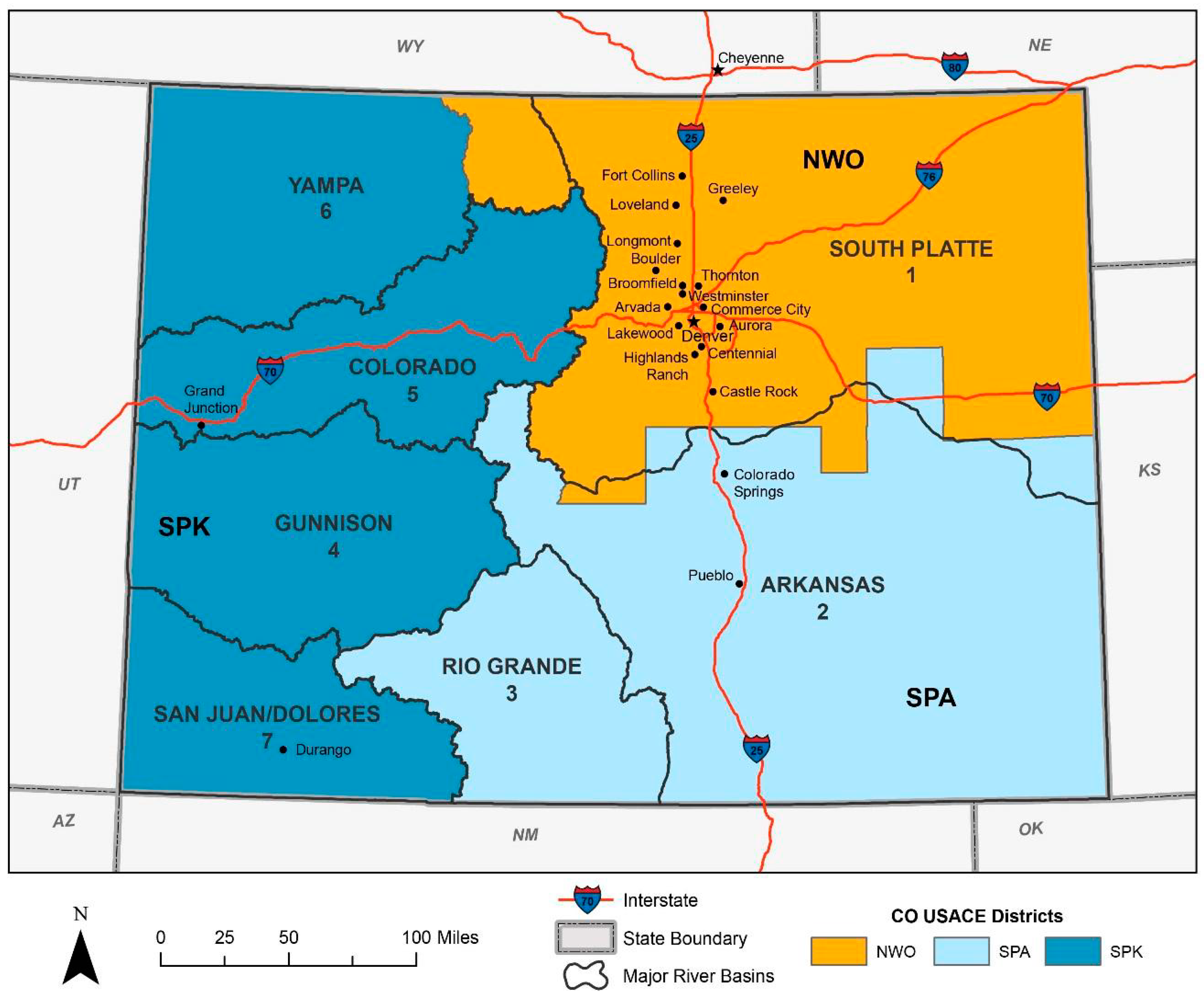
Our study area includes the entire state of Colorado, which is comprised of seven state-regulated river basins, three U.S. Army Corps of Engineers (USACE) Districts, and U.S. Ecological Protection Agency (EPA) Region 8 (Figure 1). The state of Colorado is 269,739 square kilometers in area, with a 2017 population of approximately 5.607 million persons. Relative to the 2010 decennial census, the state’s population has risen by 11.5%—compared to 5.5% for the nation as a whole during the same time span. Similarly, for the most recent period available in U.S. Census Bureau employment data (2014–2015), Colorado experienced 3.3% annual job growth compared to 2.5% nationally (U.S. Census Bureau, 2017). Thus, supporting the claims made in Section 1, Colorado is a rapidly growing state where environmental impacts related to development can be expected to continue, if not escalate, in the near future.
2.2. Data
2.2.1. Interviews with Experts, Stakeholders, Resource Managers, and Regulators
We conducted 23 semi-structured interviews (~27 h) with experts, stakeholders, resource managers, and regulators across Colorado, as well as a few experts at the national level (Appendix A). All of the information we gathered from the interviewees is anonymous and no attempt should be made to assign certain statements or opinions to any specific individual. For every piece of information gathered, we confirmed with another interviewee or published source. We also sent a draft of this article to all interviewees, collected their edits, and revised accordingly. The large diverse group of experts, stakeholders, resource managers, and regulators we interviewed allowed us to characterize the current national and state-level regulatory climate as it pertains to stream mitigation, as well as the enabling mechanisms and challenges that stream mitigation bankers will face in Colorado over the next five years.
2.2.2. Stream Impacts and Compensatory Mitigation via ORM
The OMBIL Regulatory Module (ORM2) is the second version of the national database that tracks permits that authorize work performed in, over, or under designated navigable waters; for the discharge of dredged or fill material into jurisdictional waters of the USA (WOTUS), including jurisdictional wetlands; and for ocean disposal of dredged material. This database is hereafter referred to as simply ORM. We obtained ORM data from two sources in order to check for consistencies and missing records. Our initial dataset was obtained from the Ecological Restoration Business Association (ERBA). ERBA’s data are the raw, unaltered data obtained via annual FOIA requests to USACE Headquarters, covering the period 2010 (1 October)–2016 (30 September). We obtained our second ORM dataset from a FOIA request we made to the USACE Albuquerque District (SPA), which covers the entire state of Colorado and the period 2012 (1 January)–2017 (30 June). The two datasets largely agreed, with 2206 unique records in common; however, there were 927 records that were present in SPA’s dataset that were not present in ERBA’s dataset. We also learned from a USACE ORM expert that the older annual requests will have comparatively more occurrences of errors (e.g., values for square footage instead of acres for some records). This same person assured us that the recent FOIA request we made to SPA will be more accurate. The SPA dataset also included richer information about impact type (in a field called “Worktype”), which allowed us to classify impacts into various types of land use change (e.g., transportation, development, mining). For these reasons, we only used the SPA dataset covering the period 2012–2017. Still, because there are almost certainly human-introduced errors in this dataset (e.g., data entry errors/inconsistencies), the exact values from our results should be treated as best-available estimates.
For analyses specific to stream mitigation, we only used records where the impact was: (1) permanent, (2) on a riverine/riparian Cowardin resource type, and (3) required compensatory mitigation. ORM does contain fields for mitigation required (in terms of acres, linear feet, and credits); however, due to incompleteness and inconsistencies in these units between mitigation types and across time, we used the total linear feet (LF) and acres (AC) of authorized impacts as our indicators for stream mitigation credit demand. We acknowledge that these units are not metric; however, these are the units used for mitigation credits and thus converting to metric would not be appropriate in this case.
2.2.3. Mitigation Bank Data via RIBITS
The Regulatory In lieu fee and Bank Information Tracking System (RIBITS) is a national geospatial database and repository for information on mitigation banking and in-lieu fee (ILF) programs, including mitigation credit availability and service areas for each bank/program. It was developed by USACE with support from EPA, U.S. Fish & Wildlife Service, the Federal Highway Administration, and National Oceanic and Atmospheric Administration. As soon as the data are entered into RIBITS by an USACE employee, they become available in real time on their website (https://ribits.usace.army.mil/). The RIBITS data we used were from 15 December 2017.
2.2.4. Hydrography Data and Waters of the United States (WOTUS)
We used the National Hydrography Dataset Plus (NHDPlus; v2, October 2017 update) to assess potential stream impacts from future development. To this statewide flowline dataset, we joined the value-added attributes (VAA) that contained flow classification and stream order, using the Horton-Strahler system. While actual jurisdictional determinations would have to be made after a site visit following USACE guidance, this stream order feature is useful for systematically differentiating jurisdictional WOTUS from non-jurisdictional waters over broad scales such as an entire state. NHDPlus does have a field for classifying streams as perennial, intermittent, and ephemeral; but we chose to use stream order because some intermittent streams (but not all) are jurisdictional. Based on Kampf et al. [15], many 1st-order streams would not be considered WOTUS. Thus, we took a conservative approach and only used 2nd-order streams and above for our WOTUS assessments. Our unit for most analyses was the HUC-8 watershed level because this is the most common regulatory unit for compensatory mitigation in Colorado, and usually serves as the primary service area for mitigation banks. Service areas can also be constrained by ecoregion and elevation, but these were beyond the scope of our analyses.
2.2.5. Demand-Related Data
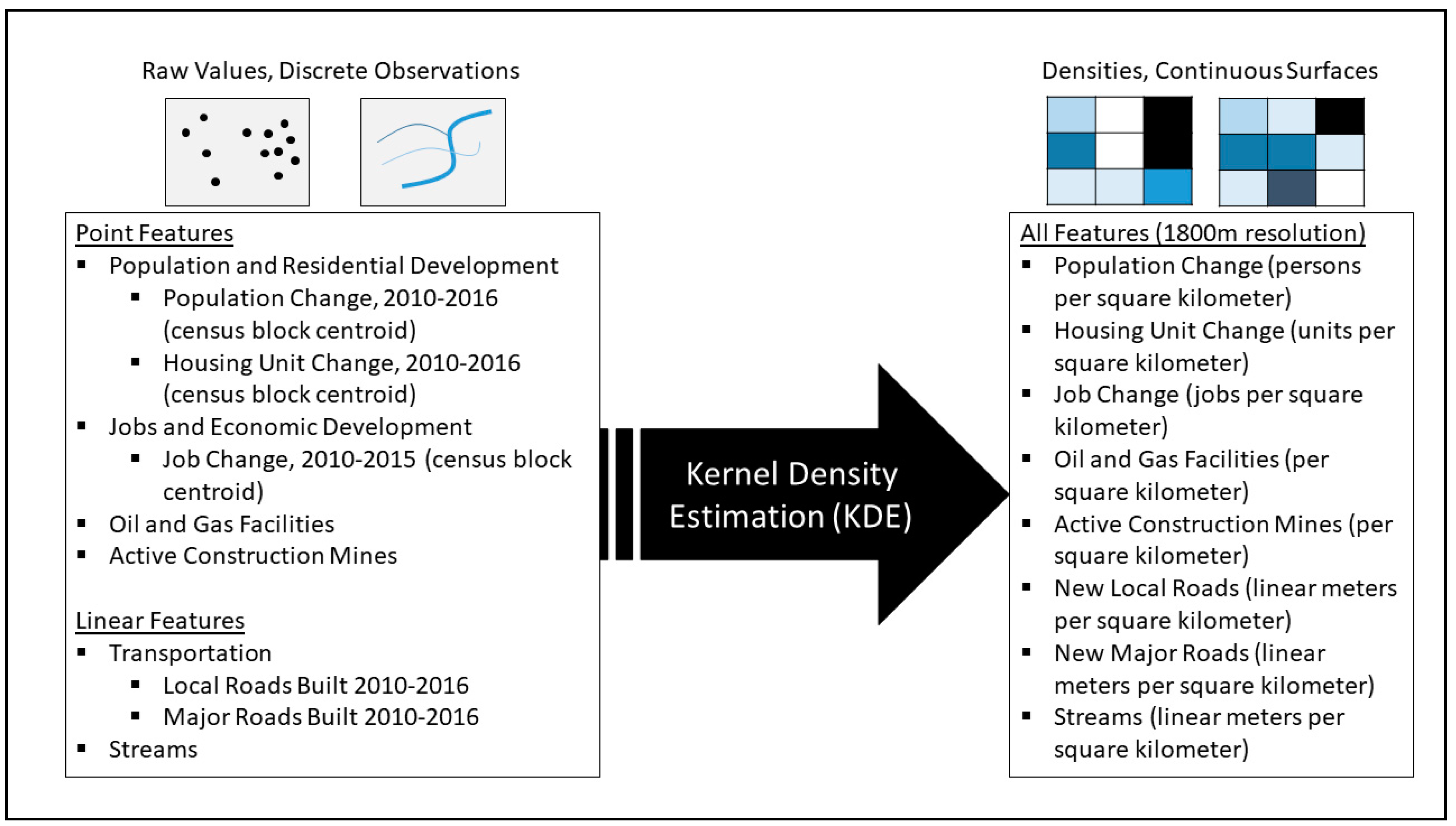
In the GIS portion of our analyses, we assessed and analyzed four drivers of stream impacts: (1) Transportation, (2) Population and Residential Development, (3) Jobs and Economic Development, and (4) Energy Development and Mining/Drilling (Table 1). Transportation data were obtained from the Colorado Department of Transportation (CDOT) on the precise locations of projects included in the agency’s 10-Year Development Plan. These projects describe road segments or related infrastructure (e.g., bridges, culverts) that are authorized to be built in the coming decade. CDOT further provides spatial data on its existing road segments. Existing segments are classified by CDOT into three types: local, major, and highway. For the former two classes of roads—local and major, which are within Colorado, while highways describe interstate roads—CDOT provides data on the year in which a segment was built, as well as its current levels of Annual Average Daily Traffic (AADT). With respect to the latter, we assume that AADT relative to designed road capacity may offer insights into where new transportation projects are likeliest to occur in the near future (i.e., to alleviate congestion).
Census block and block group level population data were obtained through Esri Business Analyst 2016. These data report counts of persons and housing units obtained from the most recent full count/decennial census (2010) at the block level. At the block group level, decennial census (2010), current (2016), and future (2021) population and housing unit figures were obtained. (Note that the estimated postcensal (2010–2016) and projected (2016–2021) growth rates provided by Esri at the block group level were applied to the 2010 census block level data to facilitate fine-resolution analyses. Block groups are, as their name suggests, groups or clusters of spatially contiguous census blocks. Adjacent blocks are grouped in order to protect individuals’ privacy when reporting sensitive socioeconomic information. In current practice, block group data are updated regularly, as new data become available from the ongoing U.S. Census American Community Survey (ACS) project. Block-level data, by contrast, are not updated between decennial censuses. For that reason, we made the simplifying assumption that change in block-level population and housing unit counts will occur at the same rate as in their parent block groups.) Changes in population and housing units over time are used below as proxies for land use change related to residential housing development.
Two publicly accessible datasets contain valuable information on patterns of jobs and economic development and, by proxy, land use changes related to commercial and industrial development. First, the Longitudinal Employer-Household Dynamics (LEHD) Origin-Destination Employment Statistics (LODES) data product from the U.S. Census Bureau provides an annual total count of jobs at the census block level of analysis. Annual job counts for each year from 2010 to 2015 (the most recent available date) were downloaded for all census blocks in the state of Colorado. These data are used below to measure changes in job counts over time, at a fine spatial resolution, as a proxy for economic development-related land uses. Second, the State of Colorado Office of Economic Development maintains a website called “Choose Colorado” (or Colorado InSite: https://choosecolorado.com/doing-business/property-search), where it markets shovel-ready sites to potential developers. As of December 2017, the website promoted 5430 undeveloped sites, nearly all of which are located in relatively close proximity to I-25 between Colorado Springs in the south and Fort Collins in the north. The spatial coordinates of these sites were obtained from Colorado InSite and used to create a point data layer in a GIS. Of the 5430 sites, 5349 (98.5%) contained valid spatial coordinates and, therefore, constituted the sample for this investigation. One attribute included in the sample data was LotSize, which describes, in acres, the spatial extent of each developable site. Because these sites are being actively promoted through a state economic development agency, they represent areas where land use changes (and, hence, environmental impacts) are likely to occur in the near to medium term. Accordingly, the locations and spatial extents of these presently vacant sites are useful proxies for future development-related land use changes.
Permitted active construction mines and active hardrock mines were acquired from the Colorado Department of Natural Resources Division of Reclamation Mining and Safety as GIS point data layers. Existing oil and gas facility locations and well lines were downloaded from the United States Geological Survey (USGS) Environment and Energy in the Rocky Mountain Area (EERMA) GIS data portal. In addition, spatial data were obtained from USGS EERMA on energy potential in two areas: geothermal and oil/gas. Collectively, these variables are used as surrogates for land use changes or land impacts related to energy development and mining and drilling.
2.3. Methodology
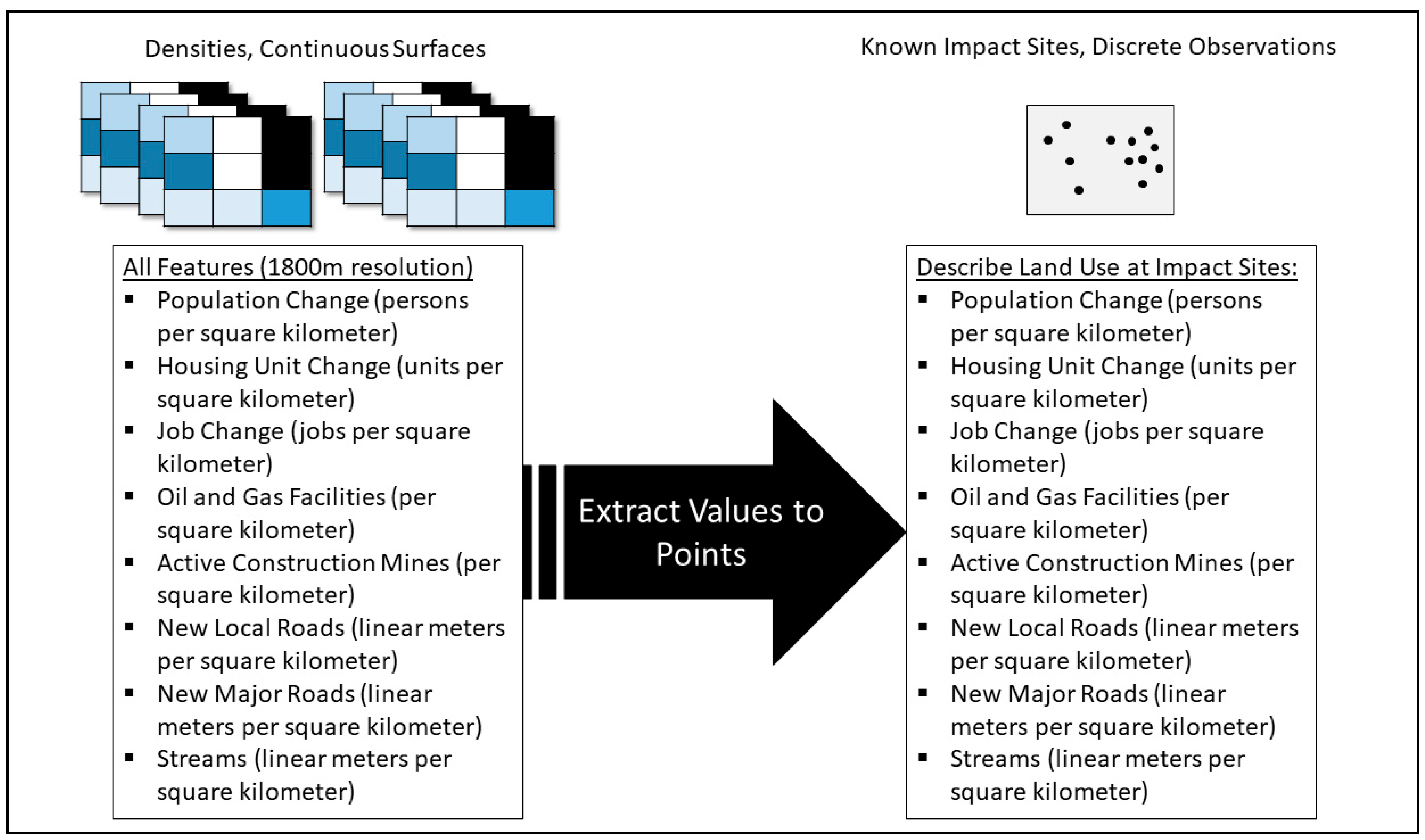
We employed a suite of spatial analytical and conventional statistical methods to map likely stream impacts in Colorado over the next five years. Demand for stream mitigation throughout was proxied using a composite index that proved to be useful for distinguishing between known: (1) locations in Colorado that registered stream impacts from 2012–2017 and those that did not, and (2) stream impact sites that required compensatory mitigation from 2012–2017 and those that did not (Appendix B). The index most readily describes a given location’s level of risk, or degree of likelihood, of experiencing stream impacts related to the pressures of growth and development. Therefore, because we assume that demand is primarily a function of (1) development-related land use changes/impacts and (2) stream density, the index acts as a proxy measure of demand.
Construction, evaluation, and implementation of the index followed a suitability analysis protocol that is fully described in Appendix B. In brief, we rasterized all vector data described in Table 1 to create input datasets with common projection, coordinate system, and spatial resolution (1800-m pixels). From there, we used map algebra to create a weighted, composite index to represent overall land use change in the presence of streams in the thematic areas of population and housing, transportation, oil/gas, and mining from 2010–2016. After considering all of the current (through 2016) variables summarized in Table 2 as candidates for the composite demand index, the final index used only those variables that took on statistically significantly different values in impact and non-impact sites. In other words, only the variables that were useful for identifying stream impacts were represented in the index. The list of these variables, and their impact strengths/degrees of influence in the index, are described in Table 3.
The value of the weighted index was compared between pixels where known stream impacts occurred through 2016 (ORM dataset) and a random sample of pixels in which there were no known impacts. Comparisons were made using both a parametric t-test for equality of means and a nonparametric Mann-Whitney/Wilcoxon test. The null hypotheses of equal means and equivalent distributions, respectively, were easily rejected. Put another way, statistical testing was used to explore whether the composite index created using the variables from Table 3 could successfully discriminate between stream impact sites and non-impact locations (Appendix B). After the tests supported this assertion, and thus the index proved to be a suitable proxy for development-related impacts/demand, we created an analogous index using projected data to quantify future demand. More specifically, the same process was used to compute an index based on the future-oriented variables enumerated in Table 4.
3. Results
3.1. Spatial Distribution of Recent Stream Impacts Requiring Compensatory Mitigation
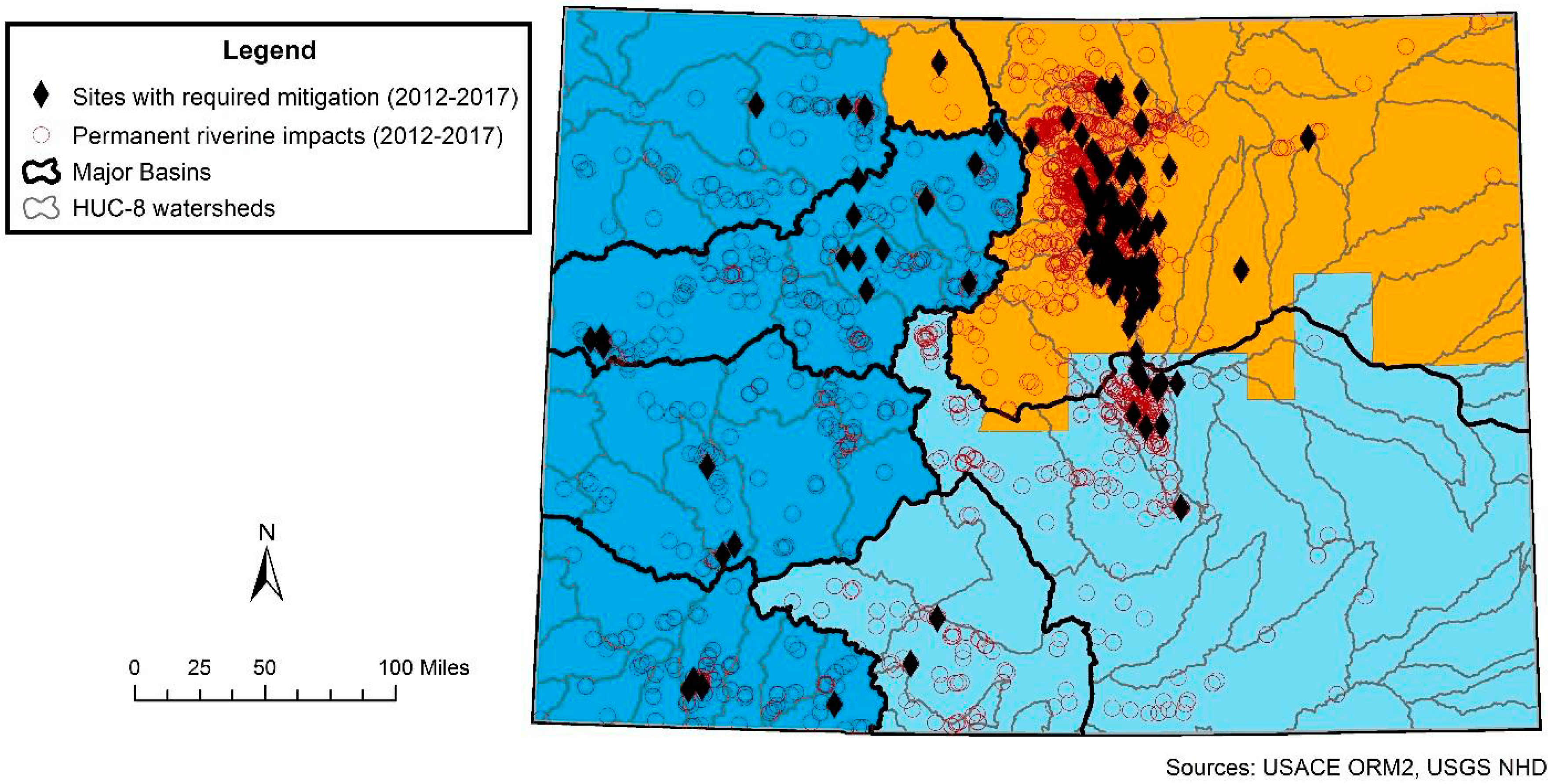
Our ORM dataset covered the period 2012–2017 and contained 14,390 records, of which 3131 were unique permits. Given the focus of this project on stream mitigation and taking into consideration that mitigation is usually only required for the loss (or permanent conversion) of an aquatic resource, we filtered this dataset to only include riverine resource types (including riparian lotic) and permanent impacts. This filtered dataset resulted in 3380 permanent riverine impacts, with the vast majority being in the South Platte River Basin around the Denver metropolitan area (Figure 2). Compensatory mitigation was required for 203 of these impacts, which includes 38,292 linear feet (LF) and 99.45 acres (AC) of permitted impacts. Of these, a little more than half (107/203) were permittee-responsible mitigation (PRM), accounting for 26,605 LF (69%) and 87.10 AC (88%). In both SPA and SPK, all permanent riverine impacts requiring mitigation were PRM. NWO had a much different situation. While there were 36,378 LF of permanent riverine impacts requiring mitigation in NWO, only 24,691 LF were PRM. That leaves 11,687 LF of non-PRM permanent riverine impacts requiring mitigation, and we are not sure how these losses were offset because there were no stream mitigation banks or ILF in NWO in Colorado. We analyze some of these impacts within the context of RIBITS in the next section.
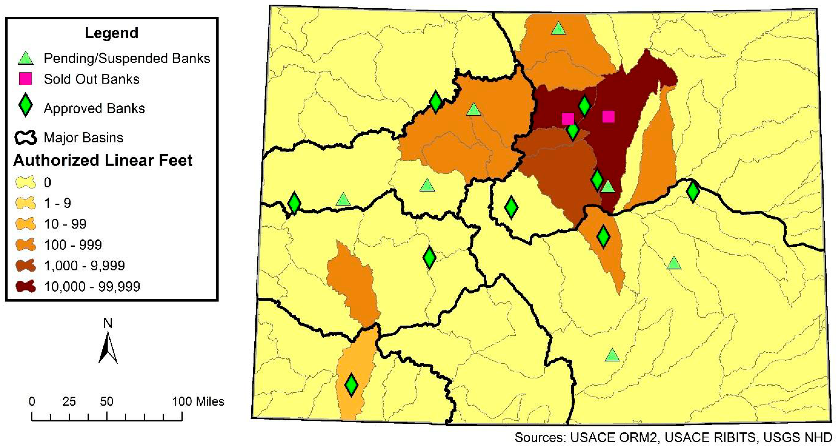
Compensatory mitigation for stream impacts in Colorado is preferred in the same HUC-8 watershed as the impact and in-kind (i.e., same aquatic resource type). With this in mind, we organized permanent riverine impacts requiring compensatory mitigation by HUC-8 watershed and resource type. To inform subsequent analyses and also to give mitigation bankers a sense of current demand, Figure 3 shows how many LF of permanent riverine impacts requiring compensatory mitigation have been authorized (by HUC-8 watershed) in Colorado for 2012–2017. As Figure 3 illustrates, there is high current demand for stream mitigation in HUC-8 watersheds surrounding the Denver metropolitan area, with two HUC-8s having more than 10,000 LF: Middle South Platte-Cherry Creek (10190003) and St. Vrain (10190005). There are several large water projects proposed for these two watersheds in the near future, which will likely add to this demand considerably. Nine other HUC-8s across Colorado have only marginal demand (<1000 LF).
In order to characterize likely stream mitigation credits for specific developments, we also summarized impacts by development type (Table 5). In terms of LF, commercial developments had the longest mean impact, followed by bank stabilization projects. Bank stabilization projects also had the greatest overall impact. What these findings suggest is that, while our composite index heavily weights commercial development activities (Appendix B), which appear to be responsible for meaningful historical stream impacts (Table 5), our final results might understate the levels of impact risk/mitigation demand in Colorado. The reason for this possibility is that data on bank stabilization projects are not readily available and were not incorporated into our index. As such, our index—which uses only commercial and residential development, transportation, and energy generation and mining proxy variables—might understate the degree and geography of near-future stream impacts in Colorado.
3.2. RIBITS and Current Supply of Mitigation Credits
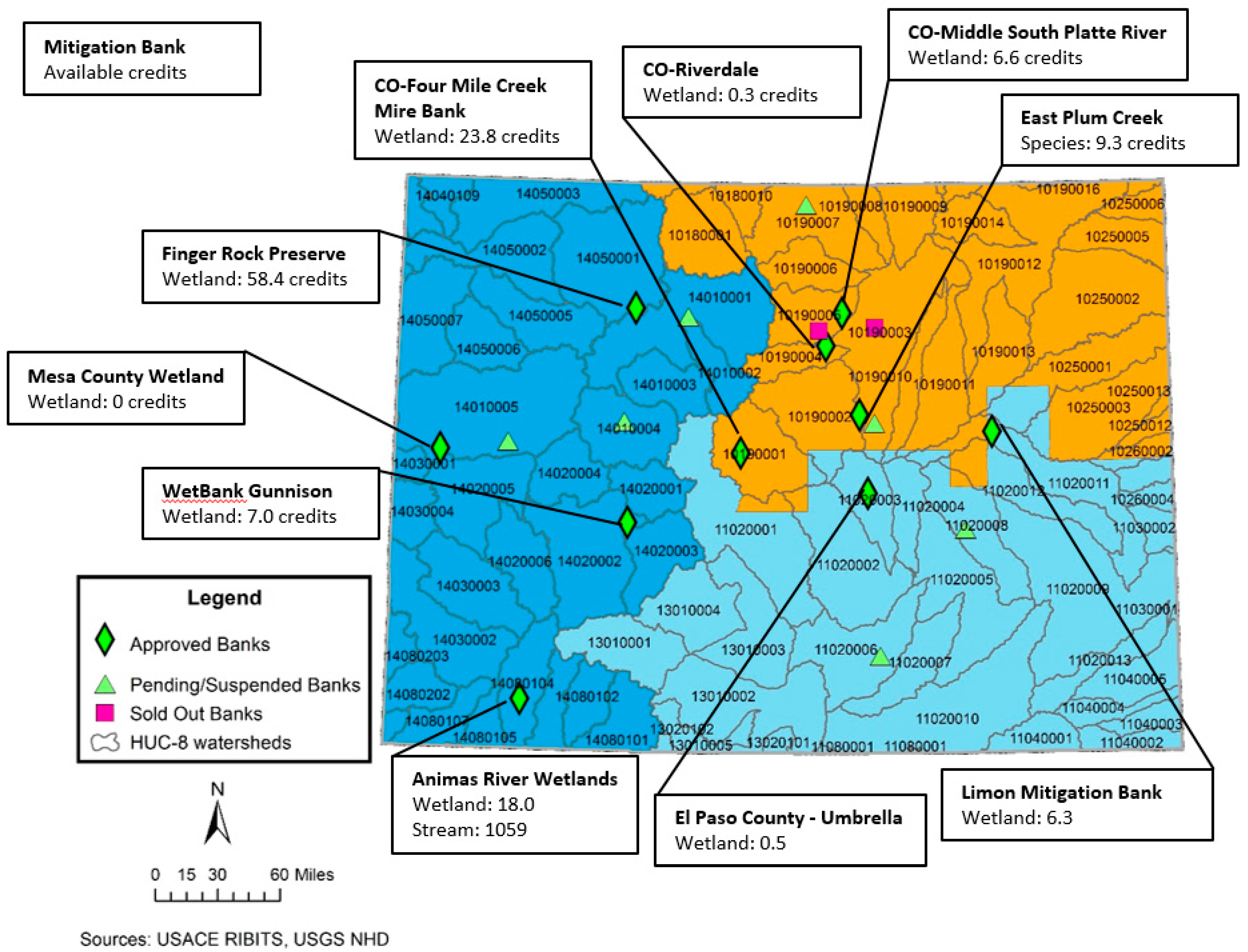
Using RIBITS to assess supply of mitigation credits, we found there have been 19 mitigation banks in Colorado (Figure 4). Of these, two have been sold out (i.e., all credits have been debited), two are suspended (no longer in compliance), and five are pending (under review or not yet in compliance). Three of the pending banks propose to offer stream credits: Cherry Creek (5500 LF perennial and 8613 LF intermittent/ephemeral to be used in the Middle South Platte-Cherry Creek watershed), Rabbit Creek (5000 LF perennial and 6300 LF intermittent to be used in the Cache La Poudre watershed), and Colorado River Conservation Reserve (9550 LF to be used in the Colorado Headwaters watershed). These LF are lengths of work, not actual proposed stream credits. The Cherry Creek and Rabbit Creek banks propose to be joint species/stream/wetland banks, providing natural, restored, and enhanced habitat for the Preble’s meadow jumping mouse. There are no ILF programs/sites in Colorado.
Only 10 mitigation banks had credits available for debiting (Figure 4). Eight of these banks are solely wetland banks, with a sum of 102.9 AC credits currently available. The East Plum Creek bank is the only species bank, with 9.3 habitat credits for the Preble’s meadow jumping mouse. The Animas River Wetlands bank is the only bank that provides stream credits (Shaded Riverine Aquatic Restored), located in southwestern Colorado with a primary service area in the Animas watershed (14080104). Out of the 2539 LF credits that were released, 1480 credits have been withdrawn, leaving 1059 credits available for debiting.
Most of the credits debited from the mitigation banks in RIBITS occurred before 2012, so we were not able to compare those with our ORM dataset. However, there are several examples of permanent riverine impacts requiring mitigation debited wetland credits. The CO-Riverdale Bank (solely a wetland bank) was used as mitigation for 10 different riverine impact permits requiring compensatory mitigation. The total authorized non-PRM impacts were 3050 LF and 1.65 AC; yet, only 1.34 credits were debited from the bank for these impacts. A similar discrepancy occurred at the CO-Middle South Platte River mitigation bank, also solely a wetland bank. The total authorized non-PRM impacts (14 different permits) were 2590 LF and 0.96 AC; yet, only 3.4 credits were debited from the bank for these impacts. Both of these banks are located in NWO, which has never had an approved stream bank. Thus, NWO has historically relied on using wetlands acre-based credits as stream offsets by multiplying the length of the stream impact by its mean width (e.g., 10 ft) to derive AC of stream impacts.
3.3. Forecasting Impacts and Demand for Stream Mitigation in Colorado Using Suitability Analysis
With the preceding points in mind, the GIS-based suitability analyses contained herein are guided by two main assumptions:
- Demand for stream mitigation is an increasing function of land use changes related to growth and development.
- Demand for stream mitigation is higher for land use changes in areas with greater concentrations of streams.
Governed by these assumptions, suitability analysis was employed to answer eight specific questions:
- Which qualitative impact types (e.g., residential development, transportation) have occurred most frequently in Colorado in the past ~5 years?
- Which qualitative impact types have required mitigation most frequently in Colorado in the past ~5 years?
- Do proxy variables for recent land use change (e.g., population change, housing unit change) differ significantly between impact sites that required mitigation and those that did not?
- Where are impacts likely to occur in Colorado in the next ~5 years?
- Which stream segments in Colorado are most at risk for impacts in the next ~5 years?
- How many linear feet (LF) of streams in Colorado are at risk for impacts in the next ~5 years?
- How many LF of streams in each HUC-8 unit in Colorado are at risk for impacts in the next ~5 years?
- Which HUC-8 units in Colorado are (most) likely to experience impactful land use change in the next ~5 years?
The most frequent types of stream impacts in Colorado during the past ~5 years were classified as Transportation (34.4%), Other (23.4%), and Structure (22.2%). Transportation impacts are most often related to road construction, improvements, and maintenance. Overwhelmingly, the most common activities in the catchall “Other” category are bank stabilization and dam maintenance, as indicated above. Some of the most common forms of Structure impacts relate to intake/outtake structures, structural maintenance, recreation, and utility lines. Because of the variety inherent in the latter two categories, Other and Structure impacts are difficult to detect with empirical data. Transportation impacts, by contrast, ought to manifest in CDOT datasets. This notion is expanded on later in this report. Noteworthy for this section, along with the interpretation of our results, is that CDOT has been thorough in acquiring permits for their impacts and providing compensatory mitigation for these impacts. This finding may bias the distribution of impact type; however, it also leads to stream mitigation demand being more predictable in Colorado.
Whereas Table 6 provides a tentative answer to research question #1, observe that the frequency of certain impact types does not necessarily speak to patterns of mitigation (research question #2). For that reason, Table 7 breaks down the generalized impacts from above by their mitigation statuses—namely, whether or not they required compensatory mitigation. As Table 7 shows, Transportation impacts remain atop the new, “mitigation required” list. However, Development takes the second position. That is, although Development impacts account for only 7.5% of all impacts from the 2010–2017 duplicate-reduced ORM dataset (Table 6), they constitute a disproportionately high 21.2% of all cases for which compensatory mitigation was required. By contrast, Other and Structural impacts account for disproportionately low shares of mitigation cases: 18.0% (mitigation cases) versus 23.4% (impacts) and 12.0% (mitigation cases) versus 22.2% (impacts), respectively (refer to Table 6 and Table 7). The upshot is that demand for stream mitigation in Colorado appears to vary more systematically with Transportation and Development impacts than with the other generalized impact types described in the ORM data. Fortunately, and as elaborated on below, these are the two categories of impacts that are most readily and consistently measurable via proxy indicators from publicly accessible secondary datasets. Most of the remaining categories—particularly the diverse Other and Structure impacts—are comparatively multivocal and, for that reason, resist consistent quantification. Two exceptions are ‘Mining and Drilling’ and ‘Energy Generation’—activities that tend to be relatively well documented by regulatory authorities. Thus, while they account for negligible percentages of overall impacts (Mining and Drilling 0.5%, Energy Generation 0.6%) and mitigation cases (Mining and Drilling 0.9%, Energy Generation 0.7%), public data are available to study these impact types. As a consequence, the four impact types that feature in the subsequent stream mitigation demand analyses are: (1) Transportation, (2) Development, (3) Mining and Drilling, and (4) Energy Generation (refer to the final column of Table 7).
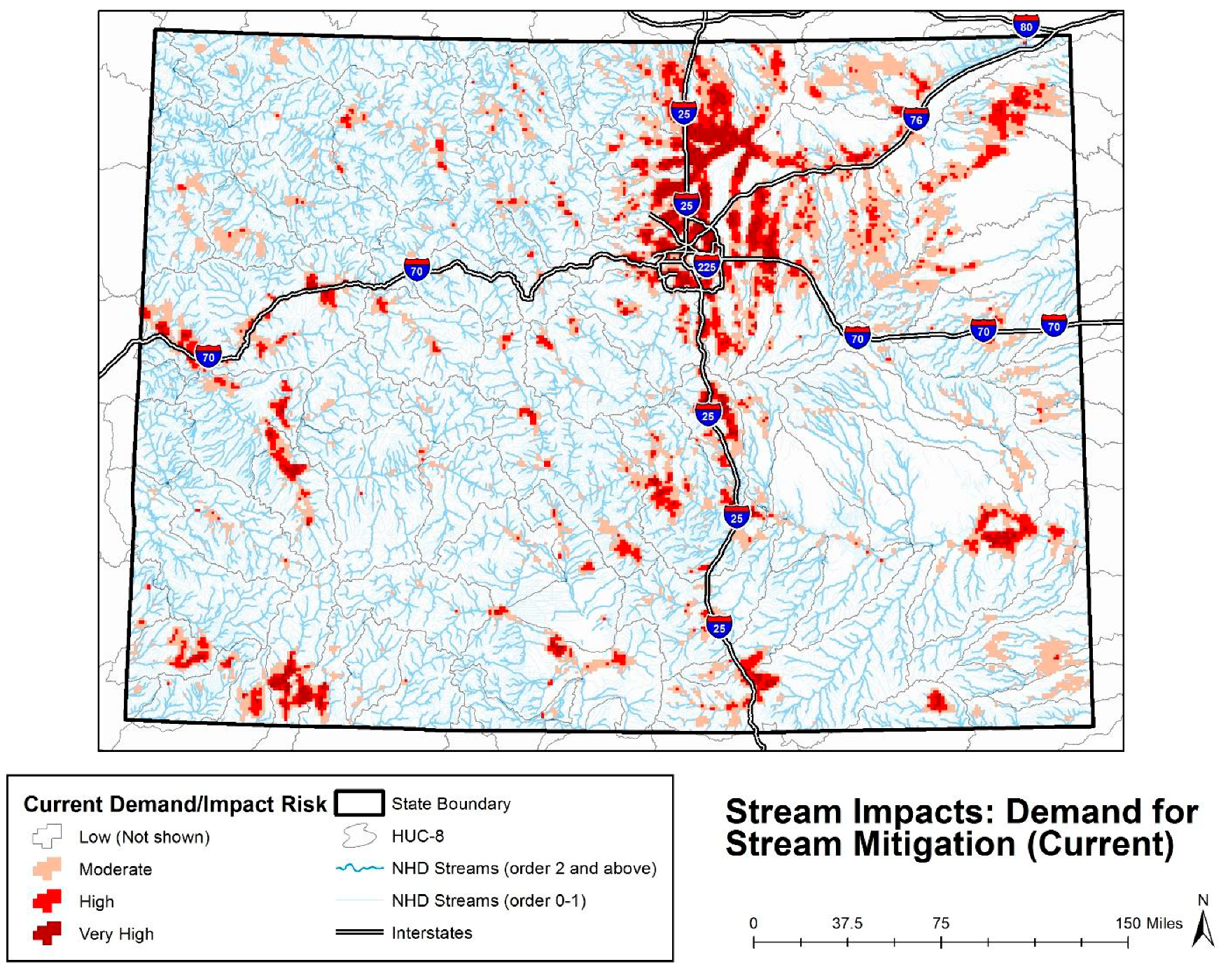
We mapped the current demand/risk levels for the entire state of Colorado (Figure 5) based on the composite index described above and detailed in Appendix B. Demand/risk levels are simplified into the following categories:
- ▪
- Low: where the demand index is within one standard deviation of the statewide average;
- ▪
- Moderate: where the demand index is between one and two standard deviations higher than the statewide average;
- ▪
- High: where the demand index is between two and three standard deviations higher than the statewide average; and
- ▪
- Very High: where the demand index is three or more standard deviations higher than the statewide average.
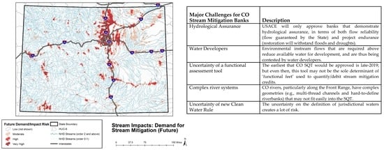
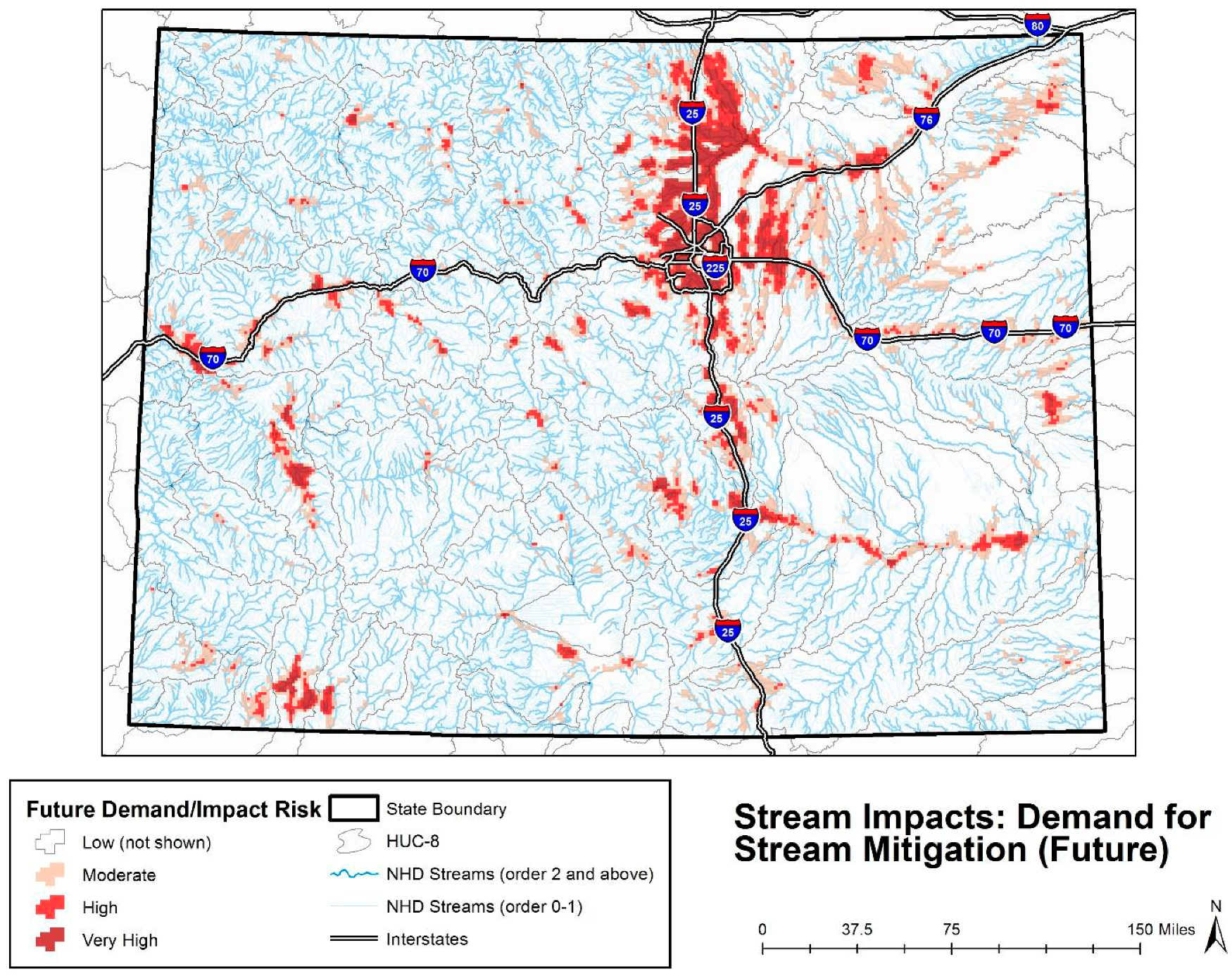
Risk levels tend to be highest in the rapidly growing I-25 urban corridor in the north-central part of the state. Figure 6 relies on the same classification scheme from above—based on standard deviations away from the statewide average of the future demand index variable (see Appendix B)—to map demand/impact risk in the near to medium term (5–10 years). In response to research question #4, which is interested in where impacts are likely to occur in the near future, Figure 6 suggests that demand/impact risk remains highest in the state’s northern urban corridor.
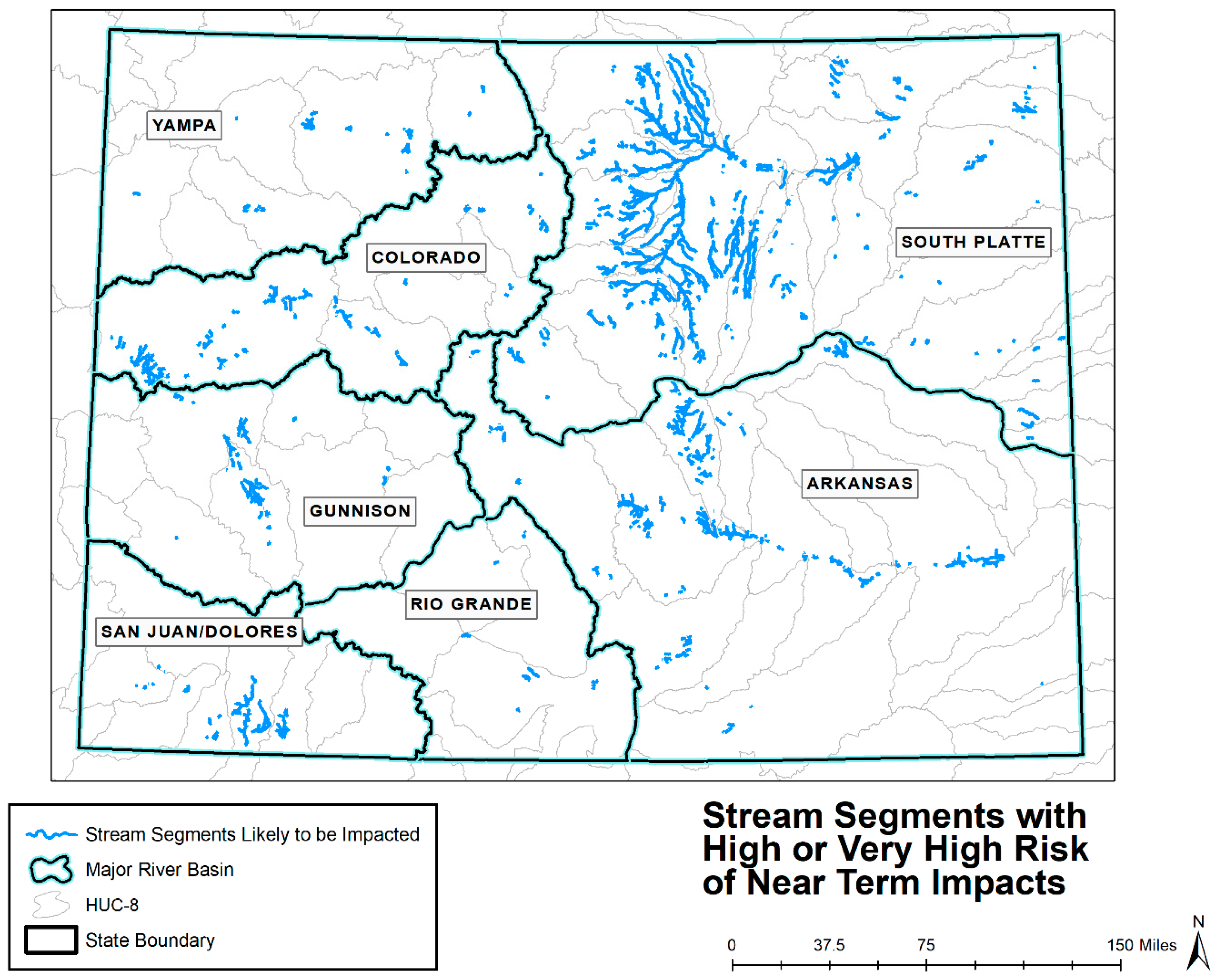
Concerning research question #5, which asks about specific stream segments at risk of being impacted in the near future, Figure 7 shows the results of a spatial intersection between stream segments (stream order 2 and above) and areas of High and Very High demand/impact risk. Table 8 provides a tentative answer to research question #6—how many LF of streams in Colorado are at high risk for impacts in the next ~5 years—by summarizing the spatial data from Figure 7.
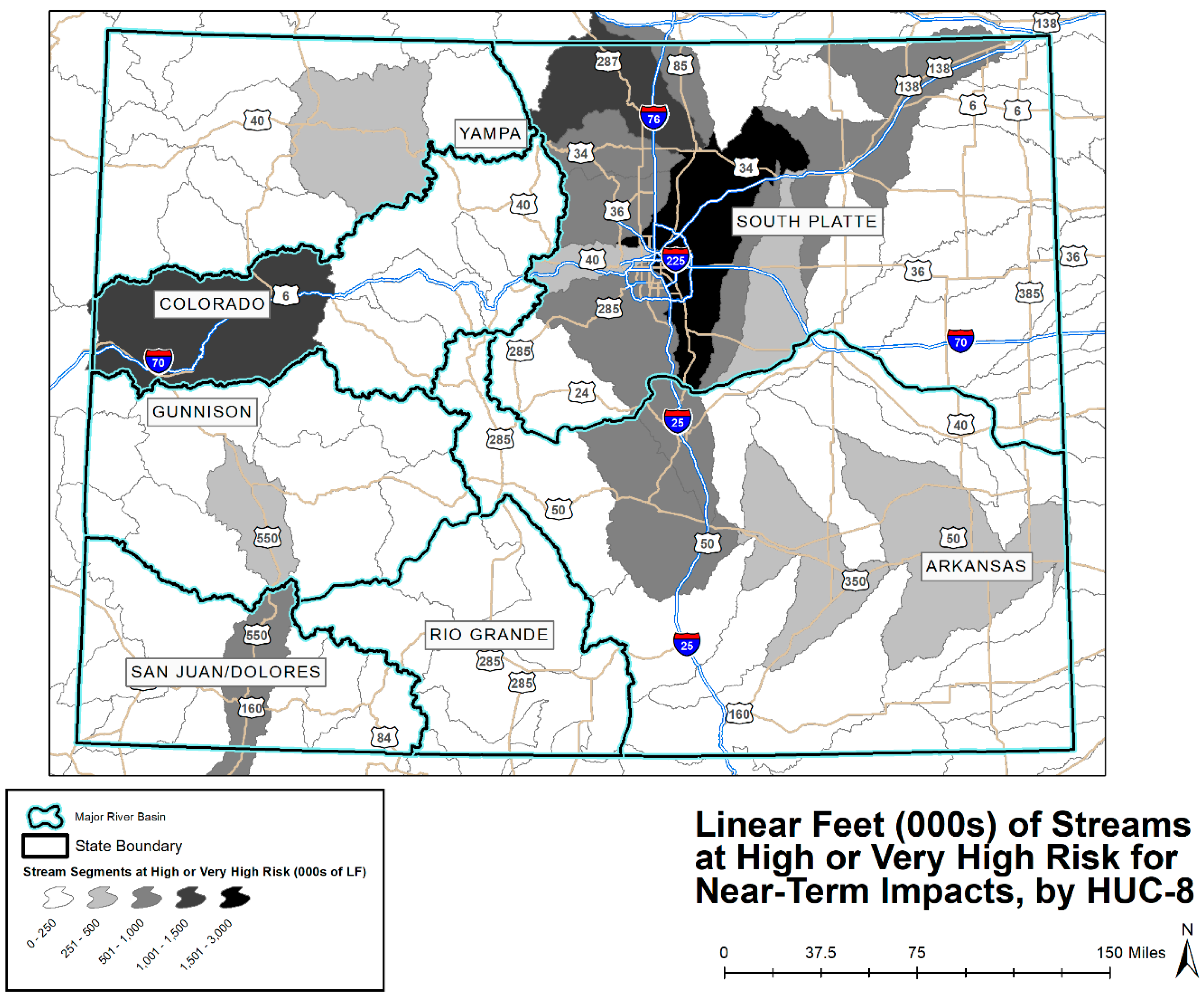
Finally, Figure 8 breaks down the aggregate information from Table 8 by HUC-8 watershed to address the final two research questions (How many LF of streams in each HUC-8 in Colorado are at high risk for impacts in the next ~5 years? and Which HUC-8 units in Colorado are (most) likely to experience impactful land use change in the next ~5 years?). Of the 89 HUC-8 watersheds that fall entirely or partially within the state of Colorado, 12 were identified as having 500,000 LF or more of their stream length associated with high impact risk/demand for stream mitigation, with three of these having greater than 1,000,000 LF (Figure 8). Eighteen of the HUC-8 watersheds had at least 10% of their stream length at high risk for impact in the near term; three of these have more than half of their stream length at high risk (Table 9).
3.4. Stakeholder Insights on Planned Stream Mitigation in Colorado
During our more than 25 h of interviews with important stakeholders across Colorado (Appendix A), we learned valuable information not only on quantification of stream mitigation credits and associated demand, but also relevant information on the regulatory climate and the social-ecological issues of establishing a new statewide program for compensatory stream mitigation. One question we asked all scientists and resource managers in the state was: What are your expectations and concerns for planned stream mitigation in Colorado? The consistent response was cautious optimism. Practically every interviewee felt that if stream mitigation will improve the health of Colorado’s degraded streams, then they are all for it as long as it is done with a landscape or watershed-scale approach, not just piecemeal. The main concern was the water rights requirements and associated obstacles. Some felt Colorado’s Division of Water Resources (DWR) and the Water Court process is too stringent when it comes to obtaining water rights for stream restoration.
Related to the water rights obstacle, everyone felt that there is not enough surface water available to maintain the environmental flows necessary to mimic the Natural Flow Regime [16] in order to ensure long-term success of the stream restoration projects. The state-level interviewees that were familiar with stream mitigation banking expressed their disappointment in the five-year success criteria for mitigation banks. One scenario that was mentioned was if riparian restoration (for stream mitigation) was performed on a Colorado River tributary where tamarisk is removed and riparian willows are planted in their place, after five years the willows would probably still be there and restoration would be considered successful. However, without long-term maintenance, tamarisk would likely invade soon after and return the fluvial system to its pre-restored state. The hope of this same individual is that stream mitigation banking would take a longer-term approach similar to conservation banking where an endowment is set up to ensure a successful restoration in perpetuity. Based on discussions with USACE representatives, it is possible (and has been put into at least one bank enabling instrument) to require these types of endowments for compensatory stream mitigation, particularly if invasive species removal is part of the restoration. USACE representatives stressed that project permanence is a requirement for mitigation bank approval. As for the five-year monitoring period for full release of mitigation credits, this can be negotiated; however, USACE is sensitive to the fact that longer monitoring periods would discourage mitigation banks, which is their preferred method of mitigation.
Another concern is the broad adoption of standardized approaches to stream restoration (e.g., Rosgen-based methods; [17]) rather than site-specific, process-based approaches. Those familiar with the Stream Quantification Tool (SQT) also expressed concern that this functional assessment tool that will be used to calculate stream impacts and credits relies too heavily on the Rosgen stream classification. Related to this concern, several interviewees felt that Colorado state agencies have prioritized engineering approaches to stream restoration over geomorphic and ecological approaches; and they fear that planned stream mitigation will reinforce and maybe even expand the engineering approach because it is easier. One interviewee pointed out that Bureau of Land Management (BLM) has been using more passive approaches to stream restoration (e.g., beaver dam analogues), and they hope that these passive approaches will be just as acceptable for stream mitigation as the more active engineering approaches that use heavy machinery and intensive earth-moving. Compensatory stream mitigation on federal land, however, is typically PRM and does not go through as rigorous of a process as private mitigation banks.
A concern from one of the state-level resource managers and one of the consultants was the potential of mitigation bankers “gaming the system,” which means either finding the most profitable sites (instead of using a functional watershed approach) or conducting restoration activities that maximize credit ratios (instead of using a site-specific functional assessment). Another concern from several interviewees was that stream mitigation bankers’ priorities would be finding profitable projects, without any concern for landscape/watershed-scale stream function. These individuals strongly recommended the State of Colorado take a watershed-based approach to stream mitigation, and not just approve suitable sites in a piecemeal fashion. Along these lines, a major concern of several interviewees was USACE’s use of linear feet as the unit of measure for assessing stream impacts and calculating stream mitigation credits.
4. Discussion
4.1. Need and Desire for Stream Mitigation Banks in Colorado
Compensatory mitigation within the context of the CWA is simply “actions taken to make permitted impacts to the aquatic ecosystem less severe” [18]. The economic growth and development across Colorado over just a short period (2012–2017) led to approximately 100 AC and 40,000 LF of authorized permanent impacts to streams requiring compensatory mitigation. The vast majority of these permitted impacts fell under Section 404 of the CWA, followed by Sections 9 and 10 of the 1899 Rivers and Harbors Act (RHA); and those impacts were the focus of this study. Stream mitigation can also be used for permitted impacts that fall under Section 303 of the CWA and Section 10 of the Endangered Species Act (ESA). Based on interviews with state regulators and resource managers, we do not expect a demand for stream mitigation for CWA Section 303 impacts in the near future. Stream mitigation for ESA impacts (or “takes”) is a possibility, particularly for endangered fish species in Colorado River tributaries (e.g., Colorado pikeminnow, humpback chub, bonytail chub, razorback sucker) and the threatened Preble’s Meadow Jumping Mouse (Zapus hudsonius preblei) along the Front Range.
The 2008 Final Rule on Compensatory Mitigation for Losses of Aquatic Resources (2008 Rule), which was released jointly by USACE (33 CFR Parts 325 and 332) and EPA (40 CFR Part 230), provides regulations for stream mitigation [14] and lays out a road map for stream mitigation moving forward in Colorado. Accordingly, much of the discussion of our results is placed within the context of the 2008 Rule. The 2008 Rule emphasizes that the first priority is to avoid impact, then minimize, and only use mitigation as a last resort. If mitigation is needed, the 2008 Rule gives preference to the method that will provide the most ‘functional lift,’ which it considers to be restoration (establishment or re-establishment of the full suite of aquatic resource functions), followed by rehabilitation (increases in most or all functions), then enhancement (lift of one or a few selected functions), and finally preservation (provides no functional lift). Thus, restoration is the generally preferred mechanism. In terms of who provides the mitigation/restoration, the 2008 Rule makes it clear that mitigation banks are the preferred provider because the offsets would occur before the impact and the mitigation project would be thoroughly vetted beforehand, compared to an in-lieu fee program (ILF) where multiple impacts may have to accumulate before mitigation is performed. One advantage of ILF, however, is that they “may be able to better target their activities to watershed needs and priorities.” Permittee-responsible mitigation (PRM) is the least preferred source of mitigation credits in the 2008 Rule.
Since the 2008 Rule, the number of mitigation banks and ILF programs across the nation has increased considerably, and there has been increasing reliance on these programs to meet compensatory mitigation requirements for permitted impacts [15]. As a result, there has been a decrease in reliance on PRM, especially on-site PRM. Since 2008, the number of stream mitigation banks has more than doubled nationwide, with most of these in the southeastern and south-central USA. The number of stream credits generated by and debited from mitigation banks has rose steadily since 2009, with more than 60 km of stream credits debited in 2014 alone [15]. In Colorado, however, there have not been any stream mitigation banks approved since 2010.
Another stipulation of the 2008 Rule is that mitigation/restoration should be in-kind. That is, stream impacts should be offset with stream credits. Most of the non-PRM permanent riverine impacts from our analysis were offset with wetland credits, which is not in-kind mitigation and results in a net loss of functional streams [9]. Given there are no ILF programs in Colorado, the other unaccounted impacts should have been offset by mitigation banks. Further, it appears that some of these permanent riverine impacts requiring mitigation may have been offset with fewer credits than permitted, although we were not able to specifically quantify. In light of all these shortcomings of the intended purpose of the CWA and the 2008 Rule, and given the intensity and extent of current and future development, there is a need and strong desire by USACE, EPA, and local resource managers for the broad-scale establishment of stream mitigation banks in Colorado. While there is a reliable market for wetland mitigation banks in almost every state (Colorado included), the number of stream mitigation banks are far fewer, and are noticeably missing from western states like Colorado [14]. We found that the lack of stream mitigation banks in western states is largely due to regulatory climate and challenges that are unique to western streams compared to eastern streams.
Overall, the results of this study have demonstrated that there is high demand for compensatory stream mitigation currently and for the near future. Practically all of the permanent riverine impacts and their associated losses of ecological functions were offset with PRM sites, which as four interviewees confirmed, do not perform as well as mitigation banks in terms of long-term ecological function. From these interviewees, we learned that mitigation banks are generally held to higher standards (compared to PRM) because (1) the permitting process for them is more rigorous, (2) they have more financial resources, (3) they have more knowledge and experience on what makes a successful project, (4) they are able and required to do more comprehensive monitoring, and (5) their reputation and financial security depends on long-term success of their projects.
While stream mitigation banking is driven by stream impacts and the regulatory agencies requiring compensatory mitigation offsets for projects, there also needs to be nearby streams in need of restoration to offset the impacts. When talking with university scientists and resource managers, a consistent comment that stood out was the degraded condition of most of Colorado’s streams, particularly in terms of their geomorphology, floodplain ecology, and overall biophysical condition. Colorado has a long and extensive history of logging, mining, and intensive agricultural practices, all of which has had many impacts on the sediment regimes, bed sediment, channel morphology, and stream ecology [19,20,21,22]. The removal of wood and beavers from rivers has had a particular degrading impact on floodplain connectivity and complexity [23]. Now, with the widespread and intensive (sub)urban development (and associated road expansions and large-scale water development projects) occurring across Colorado, sediment regimes, channel/floodplain morphology, overall water quality, and stream ecology are experiencing new threats. Several of the interviewees see stream mitigation banking as one mechanism to improve some of these degraded streams across Colorado.
4.2. Future Demand for Stream Mitigation Credits in Colorado
The exact nature of demand for stream mitigation in a jurisdiction as large as a U.S. state is partially (if not mostly) opaque, insofar as it is a function of heterogeneous and hard-to-quantify regulatory climate variables. Nevertheless, demand for stream mitigation is also, by definition, a function of stream impacts—for mitigation would not be necessary in the absence of impacts. Unlike most regulatory climate variables, many types of stream impacts are consistently detectable for large-extent study areas in empirical data. Moreover, data on historical impacts can plausibly provide insight into future impacts. Resting on this foundation, a two-part GIS-based suitability analysis was conducted to identify spaces in Colorado where growth and demand pressures are likely to result in stream impacts.
First, historical data were used to create a composite index to represent a location’s stream impact risk, or potential demand for mitigation. That index was compared between locations where known permitted impacts were observed and locations with no known impacts. In both a parametric t-test and a non-parametric Mann-Whitney/Wilcoxon test, the index proved to be significantly different between the two types of locations (Appendix B). In that sense, we argue, the index has value as a proxy for risk of development-related impacts. Second, the composite index was re-calculated using projected values of the selected input variables, where projections were obtained from Esri Business 2016. Upon spatializing the index, we identified approximately 17.5 million LF of stream segments (nearly nine percent of all stream segments in the state of Colorado) that are characterized by High (index values more than two standard deviations above the mean) or Very High (index values more than three standard deviations above the mean) levels of impact risk.
The upshot is that Colorado’s rapid growth and forward-marching economy are placing ever-greater pressures on the state’s already scarce water resources and their parent ecosystems. Stream mitigation banking represents one potential mechanism for accommodating the coming growth while alleviating some of these ecological pressures, by making mitigation a more efficient enterprise. Yet, because establishing mitigation banks requires a combination of regulatory support and entrepreneurship, as well as considerable financial risk-taking, the prospects for mitigation banking in Colorado are arguably slim absent hard empirical evidence that sufficient demand exists to make the venture mutually beneficial for bankers, developers, regulators, and all other stakeholders. Our analyses suggest that near-term development-related land use changes are likely to be impactful enough to warrant investments—both political/regulatory and financial—into mitigation banking.
4.3. Regulatory Climate in Colorado as It Pertains to Stream Mitigation
While there may be high demand for stream mitigation in Colorado, mitigation bankers will have to navigate through both the state and federal regulatory climate, both of which are experiencing significant changes related to stream mitigation. Colorado is comprised of three USACE districts (Figure 1). The Albuquerque (SPA) and Sacramento (SPK) Districts are under the South Pacific Division (SPD), whose Regional Compensatory Mitigation and Monitoring Guidelines were updated in 2015 and can be found on their Regulatory Program website (http://www.spd.usace.army.mil/Missions/Regulatory/Public-Notices-and-References/Article/558934/final-regional-compensatory-mitigation-and-monitoring-guidelines/). These 2015 SPD policies largely follow the 2008 Rule and the 2001 National Research Council Report [24] from which the 2008 Rule was based. Specific Guidance for Wetland and Stream Mitigation/Banks in the Omaha District (NWO) can be found on their Regulatory Program website (http://www.nwo.usace.army.mil/Missions/Regulatory-Program/Mitigation/), but this 2005 guidance document precedes the 2008 Rule. Based on our interviews, there is currently no plan to update NWO’s 2005 guidance document until a new Clean Water Rule is finalized and a new functional assessment is approved. With three USACE districts under two different divisions, implementing any new statewide program for stream mitigation will be complex and require a lot of people to come to an agreement.
The last key item from the 2008 Rule that is relevant to our study is the stipulation for the development and implementation of regional (e.g., state-level) protocols for quantifying functional losses (debits) and gains (credits) to aquatic resources. That is, functional metrics should be used to determine mitigation credits. While linear feet (LF) and acres (AC) have been used widely to quantify aquatic resource losses and gains, their use has been a stopgap measure until functional assessment methodologies are approved. The three USACE districts, in coordination with EPA and state agencies, are currently developing the Colorado Stream Quantification Tool (CO SQT), which is based largely on the concepts and methodology of the Stream Functions Pyramid framework [25]. Based on our interviews, this functional assessment methodology is expected to be implemented within the next year.
There are a few other federal regulatory considerations for mitigation bankers that could affect demand for stream credits. NEPA, ESA, and specific habitats are now given more consideration than in the past, which could generate more impacts requiring mitigation. There is now greater scrutiny on development activities, and greater sophistication is required by developers to prevent impacts, which could lower stream credit demand. Another federal regulation that could lower stream credit demand is the new Clean Water Rule for jurisdictional waters of the USA (WOTUS) that is currently under review. This new rule, which proposes to remove many ephemeral and intermittent stream channels in the arid/semi-arid West from WOTUS, could have particular consequences in states like Colorado where approximately 70% of all their stream length is classified as intermittent or ephemeral streams [15].
While the state regulatory climate has less influence on determination of and demand for stream mitigation credits, there are a few state-level policies/initiatives that mitigation bankers need to be aware of. Over the past decade there has been a push by most Colorado state agencies to approach stream restoration at the landscape/watershed-scale using process-based success criteria. This watershed-scale approach now has policy and funding behind it, manifested as Stream Management Plans and Watershed Protection Plans in the most recent 2015 Colorado Water Plan. The reason mitigation bankers should pay attention to these watershed plans is that the 2008 Rule has specific guidance that the USACE district engineer should evaluate proposed mitigation banks within the context of any existing watershed plans. While these plans will not likely ‘make or break’ a proposed bank site, they may influence local support for the projects.
Finally, interviewees had some interesting insights on differences between wetland mitigation vs. stream mitigation. The major difference between wetland mitigation and stream mitigation is that wetlands are largely closed systems in terms of surface water hydrology and impacts. Streams, on the other hand, are open systems where any impact can have upstream and downstream effects on channel morphology, water quality, and stream ecology. In addition to these longitudinal impacts, in-channel impacts can also have lateral impacts (riparian/floodplain), vertical impacts (groundwater), and temporal impacts (channel changes over time in response to slow and fast variables) [26,27]. Thus, any impact or mitigation to a stream can lead to multi-dimensional changes over both space and time. A major concern of several interviewees (across all sectors) was how functional assessments and stream credit generation/debiting would incorporate these indirect or secondary impacts. Thus, an important question is what will be the cumulative impacts and/or benefits for stream mitigation across Colorado’s large, diverse watersheds?
4.4. Challenges for Stream Mitigation Banks
There has only been one stream mitigation bank approved in Colorado, the Animas River Wetlands bank in the southwestern corner of the state (Figure 4). This was a unique situation in which the landowners established the bank and they were fortunate on three accounts: (1) as it was long-held family land, they had evidence showing there used to be a stream channel on their property, which allowed them to relatively easily create/restore a new channel that generated 2539 LF of stream credits; (2) they have senior water rights from the mid-1800s that are tied to their homesteaded land, providing hydrological assurance for the stream restoration; and (3) the banking instrument was approved prior to the 2015 SPD regulations and performance standards. Future proposed stream mitigation bank will not be this fortunate. Indeed, there were three proposed stream mitigation banks in Colorado at time of writing, but none were approved yet. The challenges that these pending and future stream mitigation banks face are numerous and complex (Table 10). We focus on the major ones below.
What makes it so difficult to establish an approved stream mitigation bank in Colorado? The consensus from the interviewees was that the greatest challenge, by far, is hydrological assurance. The USACE project managers I interviewed said that they have met with many mitigation bankers about numerous proposed bank sites, but only a few have resulted in complete applications because of the difficulty the banker has in providing hydrological assurance. For every stream mitigation bank, USACE requires hydrological assurances in two aspects. First, the stream needs to have a reliable flow regime that supports the ecological functions for which the project is designed. This aspect includes minimum flows for fish and other aquatic species, but also may require periodic overbank flows if riparian vegetation is part of the restoration. In Colorado, USACE requires a letter from DWR indicating that the proposed stream reach will likely have a reliable flow regime. In most circumstances, the mitigation banker will have to obtain a permanent water right, and a relatively senior one, to guarantee these required flows. Acquiring a permanent water right in Colorado is time-consuming and expensive because it is a prior-appropriation state where the vast majority of the water has already been allocated.
Even if the mitigation banker finds an opportunity to obtain a permanent water right, another challenge will be making sure there are no objections to this water right. Colorado has a state policy of limiting “buy and dry” of agricultural water rights for other uses. A majority of the senior water rights, particularly the large ones, were designated for irrigation. Thus, mitigation banks will likely be obtaining water rights that were previously used for irrigation. Keeping in mind that many other entities are securing previous agricultural water rights for uses such as urban water supply, energy development, recreation, and instream flows; there may be efforts to limit these types of water transfers, particularly from water developers. This action would trigger several consequences. First, the price of water rights would increase even further in this more active market. Second, water right transfers for instream flows may be limited or require an even more complex process than already exists. Further, there are different ‘types’ of water and some local governments/agencies (e.g., water conservancy district) may impose restrictions on how and when that water is used. The mitigation banker must also demonstrate that none of the project activities will cause an “injury” to other water rights holders. One particular concern of DWR is that restoration activities such as riparian plantings do not increase evapotranspiration water losses, which is considered to be a consumptive use that would require an additional water right. In sum, “getting the water right” for a stream mitigation bank in Colorado will require creativity, extensive planning, longer permit periods, and greater financial resources compared to most other states.
4.5. Will Stream Mitigation Banks Accomplish the Objective of Restoring and Maintaining the Chemical, Physical, and Biological Integrity of Colorado’s Waters?
The degraded state of most of Colorado’s rivers has several implications for stream mitigation and stream restoration more broadly. First, stream mitigation is only for new activities; thus, restoration or rehabilitation of stream function and health at a broad scale will require other mechanisms or policies beyond compensatory mitigation. Second, when stream impacts and potential mitigation improvements (e.g., through restoration of a nearby stream) are being assessed, we believe that more of an adaptive capacity approach should be taken. USACE and EPA stress the importance of project permanence in terms of ecological performance, but stream systems in Colorado have a wide historical range of variability from historical land uses and climate variability [20]. With many Colorado streams dependent on snowmelt runoff, many streams sensitive to small increases in air temperature (particularly within the context of coldwater fisheries), and many streams susceptible to catastrophic flooding from more intense storms, it is imperative to assess project permanence in light of these environmental changes. An adaptive capacity-based strategy fits within growing urban planning and design paradigms that call for development that creates net benefits to affected ecosystems [28] by making only context-sensitive changes that draw on the (socio-ecological) particulars of the site being developed [29].
Several scientists and resource managers expressed the optimism that there is increased interest and application of process-based restoration, particularly with regards to river floodplain complexity and connectivity. With the increasing re-introduction of large wood, beavers, and beaver dam analogues (e.g., Zeedyck dam), restoration practitioners are increasing river floodplain complexity and connectivity. To what extent could this approach be incorporated into stream mitigation regulations, policies, and protocols under the Clean Water Act? From this research, we have gained some insight into how this approach may work, but actually developing the enabling mechanisms for this approach will be fraught with challenges. Practically all scientists and resource managers interviewed recommended treating the river as a system where floodplain and channel would be considered together for purposes of both impact and mitigation. While this recommendation may be justified from an ecological perspective, it is not likely to be followed within the foreseeable future because of USACE’s jurisdiction of only in-channel impacts and mitigation, and because of all the regulations and protocols in place for stream mitigation.
An interesting topic that came up during three of our interviews was the cumulative impact of stream mitigation, since most stream mitigation is accomplished through small, reach-scale projects. To what extent do these reach-scale projects benefit the health of the entire stream system, and watershed more broadly? Section 404 permitting and its goal of minimizing individual impacts (below regulated thresholds such as 0.5 AC or 300 LF of stream) has resulted in a lot of small impacts to streams, requiring relatively small-scale mitigation and relatively few of the more ecologically rigorous Standard Permits. In fact, most of the section 404 permits do not require mitigation. So the question is: Are our streams dying from a thousand papercuts? A more extensive analysis of the ORM and RIBITS databases, beyond what we did for this study, may reveal the overall impact that the 2008 Rule, section 404 permitting, and compensatory stream mitigation has had on our nations waters.
The last issue that needs addressing, and is related to all previous discussion, is how can mitigation bankers and others in the stream restoration industry game the system, particularly in Colorado with the new tools and protocols that are being implemented. This topic was recently brought to light by Doyle and colleagues [30], where they showed that by inappropriately increasing stream length, you can increase stream credits. If the CO SQT is adopted, there are many opportunities to game the system by increasing functional feet in the spreadsheet-based calculations [31]. Functional feet, as used in the CO SQT, is most dependent on stream length, so by increasing length of restored stream, one can increase their functional feet. There is also the issue of what happens when you restore multi-thread channels, which are common in Colorado but have not been addressed by CO SQT yet. Second, and less obvious, is that the functional feet calculation is dictated by the Rosgen stream type used, which means you can change the stream type to generate more functional feet credits. Third, now with watershed location as an input variable to determine functional feet, the placement of the stream mitigation bank may be situated in a place that earns the most functional feet, but does not provide the most ecological lift to the watershed. Fourth, while the purpose of CO SQT is to reduce the amount of subjectivity and uncertainty in functional assessments, by using so many variables, uncertainty in assessments may actually increase. Specifically, uncertainty is exponentially proportional to the number of variables used in the assessment—to say nothing of the fact that some of the variables used in the CO SQT (e.g., the Rosgen stream type and basin condition) are subjective. By exposing all the ways that stream mitigation credits can be inappropriately gamed, we can hopefully prevent this from happening.
5. Conclusions
Our study has shown that there is high demand for stream mitigation banks in Colorado currently, and demand is likely to increase even further in the near future. Supply of stream mitigation banks in Colorado has not kept pace with this demand, meaning that stream impacts have not been offset with appropriate mitigation required by the CWA and the 2008 Rule. This lack of compliance should be a wake-up call for all stakeholders in Colorado concerned with stream water quality and overall ecosystem health. We have summarized many of the initiatives that are currently taking place to resolve this issue, and we recommend follow up studies to ensure that stream mitigation banks are accomplishing the objective of restoring and maintaining the chemical, physical, and biological integrity of stream systems in Colorado and beyond. Colorado is considered to be the headwaters of the USA, where its streams flow downstream to 18 other states and drain to both the Pacific and Atlantic Oceans. So, what happens in Colorado affects an entire nation and a global ecosystem.
On that note, our study marks an important first step to understanding the landscape of stream impacts (and potential for mitigation banking) in a consequential study area. Like any pilot study, however, this research is characterized by numerous limitations. For instance, while we characterized broad-scale impacts from types of development activities, we did not have enough time to investigate specific planned developments. More precisely, the trade-off we faced was largely one of breadth (in terms of geographic extent) versus depth (in terms of integrating specific development activities). Because our research questions and interests were in characterizing demand (1) at a relatively fine grain or resolution, but (2) for a large, statewide study area, we were forced to draw on data that are measured consistently across political boundaries throughout Colorado. For that reason, our methodology was built around federal (e.g., U.S. Census Bureau) and statewide (e.g., CDOT) data. Relying solely on such datasets inevitably misses the activities contained in regional, county-, city-, and community-scale plans. For example, consider that the largest single-permit impacts (in terms of functional LF of stream) appears to be dam constructions and dam elevation projects. We are aware of two proposed off-channel reservoir construction projects near Fort Collins and three proposed dam elevation projects. There will also likely be a large amount of demand for stream mitigation associated with the Northern Integrated Supply Project (NISP) and other large-scale water supply/development projects. However, to maintain our commitment to a fine resolution/large extent study that characterizes demand in a systematic and consistent fashion across the state, we were unable to incorporate these and related (specific) development plans. A future, more in-depth analysis could focus on one or two region-scale watersheds.
Next, while the preceding paragraph described the trade-off we faced between study area extent and contextual data, which forced us to use relatively broad federal and statewide datasets, an additional limitation of our demand/impact analyses is that we filtered our broad federal and state data through a single analytical process. Stated another way, we combined variables into composite measures using only one GIS-based technique. Future work is needed to test alternative methods of data combination (e.g., multiplicative combination rather than additive), and—even if our method is found to be the most suitable—conduct sensitivity analyses using multiple variable weighting schemes. Moreover, because the bulk of the data used in this study comes from federal sources, or from Colorado state sources that have analogs in most other U.S. states, it is important to replicate our work in other study areas for external validation. Although the variables we leveraged proved reliable for distinguishing (1) between known ORM impact sites and non-impact sites, as well as (2) between ORM impact sites that required mitigation and those that did not (Appendix B), this pattern of results may not hold in all study areas. Thus, the work must be carried forward and tested elsewhere. Despite these limitations, we submit that the analyses and results contained hereinbefore represent an important first step forward in developing a replicable methodological approach to assessing potential stream mitigation demand due to development pressures at the scale of an entire U.S. state.
Author Contributions
Conceptualization, J.P.J.; methodology, J.P.J., R.C.W.; software, J.P.J., R.C.W.; validation, R.C.W.; formal analysis, J.P.J., R.C.W.; investigation, J.P.J., R.C.W.; resources, J.P.J., R.C.W.; data curation, R.C.W.; writing of the original draft preparation, J.P.J., R.C.W.; writing of review and editing, J.P.J., R.C.W.; visualization, J.P.J., R.C.W.; supervision, J.P.J. R.C.W.; project administration, J.P.J.; funding acquisition, J.P.J., R.C.W.
Funding
This research was commissioned by the Meridian Institute with support from the Walton Family Foundation.
Acknowledgments
Paula Jones and Milad Korde assisted with data analyses. We also thank Adam Riggsbee, Martin Doyle, Todd Bendor, and all the interviewees in Appendix A for earlier reviews of the manuscript and answering our many questions.
Conflicts of Interest
The authors declare no conflict of interest. The Meridian Institute defined the study area and connected us with some of the stakeholders in Appendix A; but other than that, the funders had no role in the design of the study, in the collection/analyses/interpretation of data, in the writing of the manuscript, or in the decision to publish the results.
Appendix A. List of People We Interviewed to Assess Regulatory Climate and Provide Expertise on Compensatory Stream Mitigation in Colorado
- Linda Bassi, Section Chief for Stream & Lake Protection Section (Instream Flows Program), Colorado Water Conservation Board
- Brett Bovee, Regional Director at WestWater Research, LLC
- Tim Covino, Watershed Hydrologist and Stream Ecologist, Colorado State University
- Jeff Deatherage, Chief of Water Supply, Colorado Division of Water Resources
- Stephen Decker, Mitigation Banking Specialist, Omaha District, USACE
- Martin Doyle, Director of Water Policy Program, Nicholas Institute for Environmental Policy Solutions, Duke University
- Kara Hellige, Senior Project Manager, Durango Field Office, Sacramento District, USACE
- Brad Johnson, Private Consultant, Primary Investigator on the FACWet developmental team
- Sara Johnson, Executive Director of the Ecological Restoration Business Association
- Sarah Marshall, Wetland Hydrologist/Ecologist, Colorado Natural Heritage Program
- Steve Martin, Environmental Planner, USACE – Institute for Water Resources
- Julia McCarthy, Environmental Scientist, U.S. Environmental Protection Agency
- Joe McMahan, Chief-Regulatory Branch, Omaha District, USACE
- Matt Montgomery, Senior Project Manager, Grand Junction Regulatory Office, Sacramento District, USACE
- Adam Riggsbee, President, RiverBank Conservation
- Joel Sholtes, Hydraulic Engineer, Bureau of Reclamation, Lakewood, CO
- Jay Skinner, Colorado Parks & Wildlife Instream Flow Specialist
- Zach Smith, Water rights attorney, Colorado Water Trust, Denver, CO
- Allan Steinle, Chief-Regulatory Division, Albuquerque District, USACE
- Chris Sturm, Stream Restoration Coordinator, Colorado Water Conservation Board
- Luke Swan, Lead Geomorphologist and Senior Project Manager, Otak, Inc., Boulder, CO
- Reagan Waskom, Director of Colorado Water Institute
- Ellen Wohl, Fluvial Geomorphologist and Environmental Scientist, Colorado State University
Appendix B. Data Manipulation, Analytical Methods, and Intermediary Results
Appendix B.1. Data Manipulation and Analytical Methods
Prior to discussing technical procedures, it is important to point out that all of the spatial datasets described in Table 1 were obtained in vector data format. The vector data model is a means for representing real world phenomena in a GIS using what is commonly referred to as an object or discrete view of the world. Within this worldview, discrete objects are presumed to exist in otherwise empty space. For example, a given space either contains or does not contain a coffee shop. One can therefore (presumably) create a map of the distribution of coffee shops in a city by visualizing their absolute point locations (geographic coordinates) or areal spatial footprints (e.g., parcel boundaries). In the vector dataset behind such a map, the space between coffee shops is treated as empty—it is characterized by the absence of the phenomenon of interest.
Building on the foregoing example, the discrete or object view of the world is arguably appropriate for thinking singularly about phenomena such as streams, stream impacts, road segments, and the other concepts described in Table 1. However, the types of phenomena of interest to research questions #3-8—such as “land use change” and “at risk for impacts”—are more complex, in that there is no room for otherwise empty space. Put differently, land use exists everywhere and is subject to change everywhere; likewise for development risks. Accordingly, a field or continuous view of the world is seemingly better equipped to tackle the questions at hand. Within this view of the world, phenomena vary continuously across space—they exist everywhere. One means for representing continuous phenomena in a GIS is the raster data model. The raster data model effectively overlays an imaginary grid onto a study area, where all grid cells are uniform in size. The size of a grid cell is referred to as the resolution of the dataset. Each grid cell, or pixel, is assigned a value for the phenomenon of interest. In this manner, the phenomenon is represented across the entire surface of the study area.
Situated on the preceding foundations, the first step in answering the outstanding research questions is to rasterize the datasets described in the report. The reasons for doing so are implicated in Table A1, which lists the general protocols for answering research questions #3-8.

Table A1.
Approach to answering the remaining research questions.
| # | Research Question | Protocol for Answering Question |
|---|---|---|
| 3 | Do proxy variables for recent land use change (e.g., population change, housing unit change) differ significantly between impact sites that required mitigation and those that did not? | Impact sites from the ORM dataset are represented as discrete points. Raster datasets must be created to describe the continuous land use properties and changes surrounding these locations to better characterize differences, if any, between sites that required mitigation and those that did not. |
| 4 | Where are impacts likely to occur in Colorado in the next ~5 years? | Because land use change can occur anywhere, it is necessary to represent the potential for development-related land use change (and impacts) across the full extent of the study area. Raster modeling can be used to combine risk factors. |
| 5 | Which stream segments in Colorado are most at risk for impacts in the next ~5 years? | Stream (vector) data can be overlaid onto the potential development impacts (raster) data created in the previous step to identify streams that are likely to be impacted in the near future. |
| 6 | How many linear feet of streams in Colorado are at risk for impacts in the next ~5 years? | Using the output from the preceding step, the length of stream segments that intersect with high-development-risk areas can be summed. |
| 7 | How many linear of feet of streams in each HUC-8 unit in Colorado are at risk for impacts in the next ~5 years? | The total length of at-risk streams identified in response to research question #6 above can be broken down by HUC-8 unit. |
| 8 | Which HUC-8 units in Colorado are (most) likely to experience impactful land use change in the next ~5 years? | The quantitative information from the previous step can be summarized in more qualitative terms. |
Within a GIS framework, there are several ways to rasterize vector datasets. One method that is particularly well-suited to the current investigation is called kernel density estimation (KDE). KDE weights input point and line features by relevant attribute values, if any (e.g., population for a census block centroid, or linear length for a stream segment), and fits a smoothly curved surface over the discrete features. In the process, grid cells in the output raster dataset receive diminishing values the farther they are from the discrete vector objects. The exact values assigned to grid cells are, as the name of the method implies, densities, or the magnitudes of a phenomenon per unit area. For instance, a KDE output surface derived from the vector input Population Change will report the difference in the number of persons (for a given time period) per unit area in each pixel or raster grid cell within the study area.
Based on the geographic extent of the Colorado study area, we set a standard resolution for all raster datasets at 1800 m. The 1800-m resolution size was suggested by an algorithm in Esri’s ArcMap 10.5.1. For Colorado, a resolution of 1800 m translates to approximately 87,000 grid cells that are 3.24 square kilometers in area (roughly 800 acres).
Figure A1 illustrates the process for creating the eight equal-resolution raster datasets that are used below to explore differences between permitted impact sites in Colorado where mitigation was required and those where mitigation was not needed (research question #3). Four additional datasets were created and considered for these purposes: (1) distance from highways; (2) distance from rail lines; (3) hardrock mine density; and (4) oil and gas line density. However, these four datasets were not useful for distinguishing between mitigation and no-mitigation sites in relevant statistical tests. Accordingly, they were not included in the final demand analyses. For that reason, they do not merit listing in Figure A1.
Figure A1.
Using KDE to convert discrete feature distributions into equal-resolution surfaces.

The next step in addressing research question #3 was to describe land use and land use changes at the known impact sites listed in the ORM dataset. Accomplishing this task was relatively straightforward, as it merely involved extracting values from each of the newly created raster datasets (Figure A1). More specifically, each impact point from the ORM vector dataset was assigned the value of the pixel in which it fell in a given raster dataset. (Note: bilinear interpolation using adjacent pixels was employed in this process, so that the singular points used to represent impact sites are more reflective of their surroundings.) This process is illustrated in Figure A2.
Figure A2.
Characterizing land use and land use change at known impact sites.

The data described in the right-hand box of Figure A2 were used to examine differences between permitted impact sites that required mitigation and those that did not. More precisely, in light of highly skewed variable histograms, nonparametric two-sample Mann-Whitney/Wilcoxon tests were used to compare the distributions (and, roughly, the median values) of the seven impact-related variables between mitigation and no-mitigation locations. The results of these tests provided initial feedback on the extent to which the adopted proxy variables (Table A3, Figure A2) had utility for characterizing stream mitigation demand in Colorado.
Prior to moving on, note that the datasets and statistical tests discussed above can be used to describe current conditions and provide insights into the observed land use characteristics and changes that covary with known impacts and mitigation cases in Colorado. In that sense, they allowed us to understand which variables were relevant to mitigation demand based on the distribution of known mitigation cases. However, they did not allow for evaluations of research questions #4-8, which deal with probable future demand for mitigation based on expected land use characteristics and changes. Therefore, the next step was to attempt to represent projected changes in the development-related variables listed on the right-hand side of Figure A1. Toward that end, we relied on the following datasets that are referenced in Table 1:
- ▪
- Esri projected population and housing unit growth rates from 2016 to 2021;
- ▪
- Projected job growth from 2015 to 2021 (Note: 2015 is the most recent year of data available in the U.S. Census LODES dataset described above. To arrive at future job forecasts, the team relied on a type of polynomial autoregressive model in which 2015 job counts were modeled as a function of job counts in each year from 2010 to 2014, as well as the squares of those past job counts. Backwards selection revealed that only the two most recent periods (2013 and 2014), as well as their squares, had sufficient explanatory power for the 2015 job count. The parameters from a model with those four terms and an intercept were then applied iteratively to estimate job counts for 2016-2021. In other words, the job forecasts are based on somewhat of a two-period moving average. To mitigate the high uncertainty involved in the forecast process, the average of the six [moving-average] estimates were taken and used to represent “future job counts” in the demand analyses. These forecasts estimate 3.4% annual growth in jobs through 2021, which is admittedly overly optimistic relative to the 2.7% annual growth that occurred between 2010 and 2015, and the 2.2% growth rate that was expected to occur between 2016 and 2017 (Svaldi, 2016). It is recommended that future studies conduct sensitivity analyses and compare and contrast estimates from additional projection methods to quantify expected job change at the census block level. For the present pilot study, we rely on the optimistic forecasts only.);
- ▪
- USGS EERMA energy potential (gas and oil; geothermal);
- ▪
- CDOT authorized transportation projects;
- ▪
- Developable sites featured on Colorado InSite; and
- ▪
- Local and major roads currently classified by CDOT as Congested.
Assuming that existing oil and gas facilities and existing construction mines continue to operate into the future—and continue to require maintenance or perhaps even expand—the current distributions of these features were retained in the future analyses. That being said, Figure A3 illustrates the process for converting our future-related vector datasets into equal-resolution raster datasets for demand analyses. Observe that the same method (KDE) that was used above was employed here as well. Further observe that Figure A3 is effectively a future-data version of Figure A1. Relative to Figure A1, however, Figure A3 incorporates four additional datasets, which are highlighted in red.
Figure A3.
Using KDE to convert discrete feature distributions into equal-resolution surfaces (* indicates that KDE was not used to create these binary-valued raster datasets; see below.)
Figure A3.
Using KDE to convert discrete feature distributions into equal-resolution surfaces (* indicates that KDE was not used to create these binary-valued raster datasets; see below.)

Two of the red-highlighted datasets from Figure A3—CDOT authorized projects and Colorado InSite developable sites—were converted into raster surfaces using the same steps and KDE technique discussed earlier. In the former case, CDOT-authorized projects were represented as linear features in the GIS data layer. Thus, KDE was used to compute the length (in meters) of construction projects per kilometer in 1800-m resolution raster pixels. For Colorado InSite point locations, the LotSize attribute was used as a weight in KDE to compute the amount of developable land (in acres) per kilometer in the resulting raster surface. In contrast, the two remaining red-highlighted datasets from Figure A3 were treated differently. In both cases, areas of energy potential were represented by USGS EERMA as polygons. To rasterize these polygons, 1800-m resolution grid cells were assigned a value of 1 if their center fell within the polygons, and grid cells outside of the energy potential polygons were assigned a value of 0. Thus, the asterisks in Figure A3 indicate that the two flagged datasets were not generated with KDE, but were instead created by a simpler binary assignment technique.
With respect to current demand, recall that the impacts in Table A2 were taken into consideration. Further recall that Transportation and Development impacts were both regarded as “major” determinants of stream mitigation demand, given their high relative frequencies among 2012–2017 mitigation cases. Energy Generation and Mining and Drilling were both regarded as “minor” determinants on similar grounds. The selection of variables used to quantify demand (Table A2) reflects these categorizations insofar as major impacts were measured with at least two variables for every one variable used to measure minor impacts. As shown below, this choice ensured that major impacts had substantially more influence in the measures of demand than minor impacts. Still, given Assumption #2 from above, all impacts—whether major or minor—cannot be considered independent of the density of streams at the impact sites. Indeed, stream density is arguably the most important lens through which to view development impacts when assessing stream mitigation demand. With those points in mind, a four-step process was used to compute a composite index of current stream mitigation demand from the seven variables listed in Table A2 plus stream density.
Table A2.
Characterizing current demand for stream mitigation based on impacts.
| Impact Category | Impact Strength | Impact Variable(s) |
|---|---|---|
| Transportation | Major | Density of local roads built in 2010–2016 Density of major roads built in 2010–2016 |
| Development | Major | Change in population density, 2010–2016 Change in housing unit density, 2010–2016 Change in job density, 2010–2015 |
| Energy Generation | Minor | Density of oil and gas facilities |
| Mining and Drilling | Minor | Density of active construction mines |
First, the seven reclassified impact-related variables were combined additively via map algebra. Additive combination ensures that variables related to major impacts, which are represented in greater numbers, are more influential than minor impacts. Still, other functional forms—such as multiplicative combination—should be considered in future research. At any rate, summing the seven reclassified raster datasets in Step One creates a composite variable with a theoretical range from 7 to 70, though the observed range was 7 to 61. Step Two involved scaling the composite variable to make it more user-friendly. Specifically, let Ci represent the composite, current impact score for raster pixel i. The following formula was used to place C on a comparably digestible scale of 0–10:
where, again, the minimum (min) observed value of C is equal to 7 and the maximum (max) is equal to 61 in the Colorado dataset. Next, Step Three involved weighting the scaled composite index values by reclassified stream density, where original values of stream density were transformed according to the procedure described above:
While the theoretical range for the Current Demand variable is 0 to 100, the observed range for the 87,444 1800-m resolution pixels that cover the state of Colorado was 0.19 (minimum) to 98.15 (maximum), with a median of 10.55 and a mean of 13.51 (std. dev. = 10.55). Finally, the composite Current Demand measure was converted into a z-score for each pixel, by subtracting from each value the mean and dividing by the standard deviation. This step was taken to aid in classifying the demand/impact risk level of pixel cells later in the analyses (see below).
Table A3.
Characterizing future demand for stream mitigation based on impacts.
| Impact Category | Impact Strength | Impact Variable(s) |
|---|---|---|
| Transportation | Major | Density of congested local roads Density of congested major roads Density of authorized CDOT projects |
| Development | Major | Change in population density, 2016–2021 Change in housing unit density, 2016–2021 Change in job density, 2015–2021 Colorado InSite developable land density |
| Energy Generation | Minor | Density of oil and gas facilities Oil and gas potential (binary) Geothermal potential (binary) |
| Mining and Drilling | Minor | Density of active construction mines |
For future demand, we used an analogous four-step process that was applied to the reclassified variables enumerated below in Table A3. As before, variables representing major impact types strongly outnumbered variables representing minor impact types. On a similar note, observe that the two additional “energy potential” variables take on values of 0 or 1 exclusively. Therefore, while all other reclassified variables can contribute as much as 10 units to the initial composite impact score, the maximum that these (minor impact) variables can collectively contribute to the overall score is two units. That being said, future demand was computed by first summing the 11 reclassified raster datasets from Table A3. The theoretical range for this intermediate variable is 9 to 92, while the observed range was 9 to 88. Following similar steps from above, this variable (F) is placed on a scale from 0 to 10:
Note the slight tweak to the formula for future demand relative to the current demand equation. Specifically, the minimum and maximum values from the current demand variable from above, C, are used to scale future demand. The reason for doing this was to account for any residual demand or risk that might be present from land use changes that are currently operating. In practice, the adjustment does not alter the shape of the variable’s distribution in any way, since it affects all observations equally. It is simply a precaution to account for any changes that might be occurring in the present. With that in mind, future demand was quantified as:
and ultimately transformed into a z-score. The unstandardized version of the future demand variable, which has a theoretical range from 0 to 100, had an observed range from 0.95 (minimum) to 100 (maximum), with a median of 10.48 and a mean of 13.60 (std. dev. = 11.31).
Prior to relying the future demand variable, it is important to first demonstrate that the indices described hereinbefore are useful proxies for stream mitigation demand. To make this case, the current demand index was extracted for each of the known impact sites from the ORM dataset (refer to the process described in Figure A2). By way of a standard two-sample t-test (for differences in means) and a two-sample Mann-Whitney/Wilcoxon test (for differences in distributions and, roughly, medians), we were able to understand the extent to which the demand index differentiated between impact sites that required mitigation and those that did not.
Appendix B.2. Intermediary Results
The results from two-sample Mann-Whitney/Wilcoxon tests for differences in the seven impact-related variables described on the right-hand side of Figure A2 are presented in Table A4, alongside corresponding t-tests. In all cases, the sample of impacts that required mitigation were found to be different than the sample of impacts that did not require mitigation. This pattern of findings suggests that the selected variables have value for distinguishing between impacts that require mitigation and those that do not.
Given the pattern of significant differences presented in Table A4, it is reasonable to conclude that the Current Demand index—which is a composite of the seven variables from Table A3 that interacted with stream density—has value as a proxy for detecting stream impacts, and by extension, is a useful proxy for stream mitigation demand. To test this assertion, we selected all of the 1800-m resolution raster pixels in which impact points from the ORM dataset can be found. (NB: There are 1206 such pixels, indicating that most of the permitted impacts occur in close proximity.) From there, a random sample of 2412 pixels (twice the number of impact pixels) was drawn from the raster dataset. Table A5 presents the results from a t-test and a Mann-Whitney/Wilcoxon test that compares the Current Demand index for known impact points relative to randomly selected (non-impact) points throughout the state of Colorado. As expected, the index takes on substantially higher values at known impact sites.
Table A4.
Results of statistical tests for development variables.
| Mitigation Not Required (n = 4602) | Mitigation Required (n = 449) | |||
|---|---|---|---|---|
| Variable | Mean | Median | Mean | Median |
| Density of local roads built in 2010–2016 | 32.66 | 6.21 | 46.44 *** | 28.92 *** |
| Density of major roads built in 2010–2016 | 6.13 | 0.36 | 6.65 | 1.70 *** |
| Change in population density, 2010–2016 | 38.02 | 7.57 | 60.96 *** | 48.05 *** |
| Change in housing unit density, 2010–2016 | 13.70 | 3.80 | 19.75 *** | 16.38 *** |
| Change in job density, 2010–2015 | 37.38 | 1.78 | 95.78 *** | 7.87 *** |
| Density of oil and gas facilities | 0.10 | 0.02 | 0.13 *** | 0.05 *** |
| Density of active construction mines | 2.24 | 0.68 | 2.65 * | 0.82 ** |
*** p < 0.001 ** p < 0.010 * p < 0.050 (asterisks in Mean column refer to t-tests; those in Median column refer to Mann-Whitney/Wilcoxon tests).
Table A5.
Results of statistical tests for modeled demand.
| No Impact (2010–2016) Present in Location (n = 2392) | Location of Known (2010–2016) Stream Impact (n = 1206) | |||
|---|---|---|---|---|
| Variable | Mean | Median | Mean | Median |
| Current Demand | 13.07 | 10.37 | 33.45 *** | 31.11 *** |
| Current Demand (z-score) | −0.04 | −0.30 | 1.89 *** | 1.67 *** |
*** p < 0.001 (asterisks in Mean column refer to a t-test; in Median column they refer to a Mann-Whitney/Wilcoxon test) NB: 20 of the randomly selected pixels fell partially over the Colorado state boundary, and therefore had missing/null index values.
Apart from supporting the claim that the land use-related variables employed in this study are suitable for detecting stream impacts, the results from Table A5 contain an interesting insight. Namely, on average, locations of stream impacts take on a Current Demand value nearly two standard deviations above the variable’s mean (compared to an average z-score of −0.30 for all other sites, and a mean of 0 for the full dataset). Using this observation as a jumping-off point, the following scheme was adopted to characterize demand (or, equivalently, risk of stream impacts):
- ▪
- Low: Current Demand (z-score) < 1.0
- ▪
- Moderate: 1.0 ≤ Current Demand (z-score) < 2.0
- ▪
- High: 2.0 ≤ Current Demand (z-score) < 3.0
- ▪
- Very High: Current Demand (z-score) ≥ 3.0
References
- Murphy, J. Chart: Colorado Is the Second-Fastest Growing State in the U.S. The Denver Post. 7 July 2016. Available online: https://www.denverpost.com/2016/2007/2007/colorado-second-population-growth-2015/ (accessed on 8 March 2018).
- Weissmann, J. The Fastest-Growing States in America (and Why They‘re Booming). The Atlantic. 12 December 2012. Available online: https://www.theatlantic.com/business/archive/2012/2012/the-fastest-growing-states-in-america-and-why-theyre-booming/266541/ (accessed on 8 March 2018).
- Svaldi, A. Colorado Economy Set for Continued Growth in 2017, Despite Worker Shortages. The Denver Post. 5 December 2016. Available online: https://www.denverpost.com/2016/2012/2005/colorado-economy-growth-2017/ (accessed on 8 March 2018).
- U.S. Department of Energy. 2017 U.S. Energy and Jobs Report State Charts. 2017; p. 32. Available online: https://energy.gov/sites/prod/files/2017/2001/f2034/2017%2020US%2020Energy%2020and%2020Jobs%2020Report%2020State%2020Charts%2202_2010.pdf (accessed on 8 March 2018).
- Eason, B. Colorado’s Growing Pains: From Roads to Water, Here Are 5 Key Issues as the State’s Population Swells. The Denver Post. 15 October 2017. Available online: https://www.denverpost.com/2017/2010/2015/colorado-growing-population-issues/ (accessed on 8 March 2018).
- Weaver, R.; Bagchi-Sen, S.; Knight, J.; Frazier, A.E. Shrinking Cities: Understanding Urban Decline in the United States; Routledge: New York, NY, USA, 2016; p. 245. [Google Scholar]
- Leo, C.; Anderson, K. Being realistic about urban growth. J. Urban Aff. 2006, 28, 169–189. [Google Scholar] [CrossRef]
- Daly, H.E.; Farley, J. Ecological Economics: Principles and Applications; Island Press: Washington, DC, USA, 2004; p. 450. [Google Scholar]
- BenDor, T.; Sholtes, J.; Doyle, M.W. Landscape characteristics of a stream and wetland mitigation banking program. Ecol. Appl. 2009, 19, 2078–2092. [Google Scholar] [CrossRef] [PubMed]
- Davis, S.K. The politics of water scarcity in the western states. Soc. Sci. J. 2001, 38, 527–542. [Google Scholar] [CrossRef] [Green Version]
- Peterson, J. Water Experts Prepare for Colorado’s Population Boom. The Durango Herald. 25 June 2017. Available online: https://durangoherald.com/articles/167803 (accessed on 8 March 2018).
- BenDor, T.; Stewart, A. Land Use Planning and Social Equity in North Carolina’s Compensatory Wetland and Stream Mitigation Programs. Environ. Manag. 2011, 47, 239–253. [Google Scholar] [CrossRef] [PubMed]
- Lave, R.; Robertson, M.M.; Doyle, M.W. Why You Should Pay Attention to Stream Mitigation Banking. Ecol. Restor. 2008, 26, 287–289. [Google Scholar] [CrossRef]
- Institute for Water Resources. The Mitigation Rule Retrospective: A Review of the 2008 Regulations Governing Compensatory Mitigation for Losses of Aquatic Resources; USACE, 2015-R-03; Institute for Water Resources: Alexandria, VA, USA, 2015. Available online: https://www.iwr.usace.army.mil/Portals/70/docs/iwrreports/2015-R-03.pdf (accessed on 18 January 2019).
- Kampf, S.K.; Puntenney, K.; Martin, C.; Weber, R.; Gerlich, J.; Hammond, J.C.; Lefsky, M.A. Controls on streamflow intermittence in the Colorado Front Range. In Proceedings of the American Geophysical Union Fall Meeting, New Orleans, LA, USA, 11–15 December 2017. [Google Scholar]
- Poff, N.L.; Allan, J.D.; Bain, M.B.; Karr, J.R.; Prestegaard, K.L.; Richter, B.D.; Sparks, R.E.; Stromberg, J.C. The natural flow regime. Bioscience 1997, 47, 769–784. [Google Scholar] [CrossRef]
- Rosgen, D.L. Watershed Assessment of River Stability and Sediment Supply, 2nd ed.; Wildland Hydrology: Fort Collins, CO, USA, 2008; p. 684. [Google Scholar]
- Hough, P.; Robertson, M. Mitigation under Section 404 of the Clean Water Act: Where it comes from, what it means. Wetl. Ecol. Manag. 2009, 17, 15–33. [Google Scholar] [CrossRef]
- Allan, J.D. Landscapes and Riverscapes: The Influence of Land Use on Stream Ecosystems. Annu. Rev. Ecol. Evol. Syst. 2004, 35, 257–284. [Google Scholar] [CrossRef] [Green Version]
- Wohl, E.E. Rivers in the Landscape: Science and Management; Wiley-Blackwell: Oxford, UK, 2014; p. 330. [Google Scholar]
- Wohl, E. Wide Rivers Crossed the South Platte and the Illinois of the American Prairie; University Press of Colorado: Boulder, CO, USA, 2013; p. 408. [Google Scholar]
- Wohl, E. Virtual Rivers: Lessons from the Mountain Rivers of the Colorado Front Range; Yale University Press: New Haven, CT, USA, 2001; p. 224. [Google Scholar]
- Wohl, E.; Lininger, K.B.; Fox, M.; Baillie, B.R.; Erskine, W.D. Instream large wood loads across bioclimatic regions. For. Ecol. Manag. 2017, 404, 370–380. [Google Scholar] [CrossRef]
- National Research Council. Compensating for Wetland Losses under the Clean Water Act; The National Academies Press: Washington, DC, USA, 2001; p. 348. [Google Scholar]
- Harman, W.; Starr, R.; Carter, M.; Tweedy, K.; Clemmons, M.; Suggs, K.; Miller, C. A Function-Based Framework for Stream Assessment and Restoration Projects; EPA 843-K-12-006; U.S. Environmental Protection Agency, Office of Wetlands, Oceans, and Watersheds: Washington, DC, USA, 2012.
- Ward, J.V. The four-dimensional nature of lotic ecosystems. J. N. Am. Benthol. Soc. 1989, 8, 2–8. [Google Scholar] [CrossRef]
- Julian, J.P.; Podolak, C.J.P.; Meitzen, K.M.; Doyle, M.W.; Manners, R.B.; Hester, E.T.; Ensign, S.; Wilgruber, N.A. Shaping the physical template: Biological, hydrological, and geomorphic connections in stream channels. In Stream Ecosystems in a Changing Environment; Jones, J.B., Stanley, E.H., Eds.; Elsevier: London, UK, 2016; pp. 85–133. [Google Scholar]
- Garrard, G.E.; Williams, N.S.G.; Mata, L.; Thomas, J.; Bekessy, S.A. Biodiversity Sensitive Urban Design. Conserv. Lett. 2018, 11, e12411. [Google Scholar] [CrossRef]
- Hester, R.T. Design for Ecological Democracy; MIT Press: Cambridge, CA, USA, 2006; p. 528. [Google Scholar]
- Doyle, M.W.; Singh, J.; Lave, R.; Robertson, M.M. The morphology of streams restored for market and nonmarket purposes: Insights from a mixed natural-social science approach. Water Resour. Res. 2015, 51, 5603–5622. [Google Scholar] [CrossRef] [Green Version]
- Swan, L.; Beeby, J.; Smull, E.; Bledsoe, B.; Gurnee, G.; Auckland, J. Wyoming Stream Quantification Tool Field Testing and Review; Meridian Institute: Washington, DC, USA, 2017; p. 58. [Google Scholar]
Figure 1.
Colorado study area with state and federal regulatory boundaries relevant to stream mitigation. The three USACE Districts are Omaha (NWO), which is under the Northwest Division, and Albuquerque (SPA) and Sacramento (SPK), which are under the South Pacific Division (SPD). USACE field offices are located in Denver, Pueblo, Durango, and Grand Junction.

Figure 2.
Permanent riverine impacts and sites with required compensatory mitigation in Colorado for 2012–2017. The Colorado USACE districts are NWO (orange), SPK (dark blue), and SPA (light blue).
Figure 2.
Permanent riverine impacts and sites with required compensatory mitigation in Colorado for 2012–2017. The Colorado USACE districts are NWO (orange), SPK (dark blue), and SPA (light blue).

Figure 3.
Authorized linear feet (LF) of permanent riverine impacts requiring compensatory mitigation by HUC-8 watershed in Colorado for 2012–2017. Mitigation banks have been added for context.
Figure 3.
Authorized linear feet (LF) of permanent riverine impacts requiring compensatory mitigation by HUC-8 watershed in Colorado for 2012–2017. Mitigation banks have been added for context.

Figure 4.
Mitigation bank locations across Colorado and current supply of mitigation credits, as reported by RIBITS on 15 December 2017.
Figure 4.
Mitigation bank locations across Colorado and current supply of mitigation credits, as reported by RIBITS on 15 December 2017.

Figure 5.
Current stream impacts/demand for mitigation in Colorado.

Figure 6.
Projected stream impacts/demand for mitigation in Colorado.

Figure 7.
Stream segments with high or very high risk of near-term impacts.

Figure 8.
Risk/demand assessment for stream mitigation in Colorado by HUC-8 watershed.

Table 1.
Overview of demand-related data.
| Category | Dataset | Key Variable(s) | Level of Analysis | Coverage |
|---|---|---|---|---|
| Population and Residential Development | Esri data | -Population (current and future) -Housing units (current and future) | Block/Block group | Statewide |
| Jobs and Economic Development | LODES | -Job count (current; future to be forecasted) | Block/Block group | Statewide |
| Colorado InSite | -Shovel ready sites | Point/impact area | Statewide | |
| Transportation | CDOT planned projects | -Planned transportation projects | Line/impact area | Statewide |
| CDOT road segments | -Road type (highway, major, local) -Year built (for major and local roads only) -Congested (Yes or No) | Line/road segment | Statewide | |
| Energy Development and Mining and Drilling | USGS EERMA Colorado Division of Reclamation Mining & Safety | -Existing oil and gas facilities -Permitted hard rock and active construction mines -Future energy development | Point (current) Area (future) | Statewide |
Table 2.
Selected summary of demand-related data.
| Variable | Summary | |
|---|---|---|
| Population | 2010 Total: | 5,029,196 persons |
| 2016 Estimate: | 5,425,481 persons | |
| 2021 Projection: | 5,831,123 persons | |
| Housing | 2010 Total: | 2,212,898 units |
| 2016 Estimate: | 2,359,070 units | |
| 2021 Projection: | 2,522,289 units | |
| Jobs | 2010 Total: | 2,129,886 jobs |
| 2015 Total: | 2,441,882 jobs | |
| Transportation | Highways: | 14,649.4 km |
| Major Roads: | 27,896.6 km | |
| 13.0% Congested | ||
| 1% with YearBuilt >= 2012 | ||
| Local Roads: | 105,945.2 km | |
| 15.2% Congested | ||
| 1.3% with YearBuilt >= 2012 | ||
| Planned Roads: | 1774.1 km | |
| Oil/Gas | Facilities: | 13,416 features |
| Directional Lines: | 8755.0 km | |
| Mining | Hardrock Mines: | 110 features (25,052.5 affected acres) |
| Construction Mines: | 826 features (83,104.4 affected acres) | |
| Streams | Order ≥ 2: | 60,443.7 km |
Table 3.
Characterizing current demand for stream mitigation based on impacts.
| Impact Category | Impact Strength | Impact Variable(s) |
|---|---|---|
| Transportation | Major | Density of local roads built in 2010–2016 Density of major roads built in 2010–2016 |
| Development | Major | Change in population density, 2010–2016 Change in housing unit density, 2010–2016 Change in job density, 2010–2015 |
| Energy Generation | Minor | Density of oil and gas facilities |
| Mining and Drilling | Minor | Density of active construction mines |
Table 4.
Characterizing future demand for stream mitigation based on impacts.
| Impact Category | Impact Strength | Impact Variable(s) |
|---|---|---|
| Transportation | Major | Density of congested local roads Density of congested major roads Density of authorized CDOT projects |
| Development | Major | Change in population density, 2016–2021 Change in housing unit density, 2016–2021 Change in job density, 2015–2021 Colorado InSite developable land density |
| Energy Generation | Minor | Density of oil and gas facilities Oil and gas potential (binary) Geothermal potential (binary) |
| Mining and Drilling | Minor | Density of active construction mines |
Table 5.
Permanent riverine impacts in Colorado (2012–2017) requiring compensatory mitigation by development type. Values of linear feet (LF) and acres (AC) are the impacted length/area requiring mitigation, not the mitigation credits that were debited.
Table 5.
Permanent riverine impacts in Colorado (2012–2017) requiring compensatory mitigation by development type. Values of linear feet (LF) and acres (AC) are the impacted length/area requiring mitigation, not the mitigation credits that were debited.
| Work Type | LF Statistics | AC Statistics |
|---|---|---|
| Residential development | Min = 0 | Min = 0 |
| Max = 800 | Max = 1.47 | |
| Median = 0 | Median = 0.25 | |
| Mean = 99.4 | Mean = 0.39 | |
| Sum = 1392 | Sum = 5.51 | |
| Commercial development | Min = 0 | Min = 0.13 |
| Max = 3700 | Max = 0.95 | |
| Median = 0 | Median = 0.47 | |
| Mean = 740 | Mean = 0.56 | |
| Sum = 3700 | Sum = 2.81 | |
| Road Improvement | Min = 0 | Min = 0.01 |
| Max = 5300 | Max = 32.50 | |
| Median = 0 | Median = 0.02 | |
| Mean = 259.6 | Mean = 2.00 | |
| Sum = 5452 | Sum = 42.06 | |
| Culvert and Non-bridge crossing | Min = 0 | Min = 0 |
| Max = 400 | Max = 0.44 | |
| Median = 0 | Median = 0.05 | |
| Mean = 20 | Mean = 0.10 | |
| Sum = 400 | Sum = 1.97 | |
| Bridge Construction/Maintenance | Min = 0 | Min = 0 |
| Max = 1300 | Max = 2.56 | |
| Median = 0 | Median = 0.06 | |
| Mean = 118.9 | Mean= 0.25 | |
| Sum = 2854 | Sum = 6.00 | |
| Mitigation and Bank stabilization | Min = 0 | Min = 0 |
| Max = 2647 | Max = 8.6 | |
| Median = 0 | Median = 0.01 | |
| Mean = 298.2 | Mean= 0.34 | |
| Sum = 16700 | Sum = 18.94 | |
| Energy generation and Mining | Min = 0 | Min = 0.02 |
| Max = 0 | Max = 0.63 | |
| Median = 0 | Median = 0.21 | |
| Mean = 0 | Mean = 0.24 | |
| Sum = 0 | Sum = 1.70 | |
| Dam construction and maintenance | Min = 0 | Min = 0 |
| Max = 750 | Max = 1.7 | |
| Median = 0 | Median = 0.04 | |
| Mean = 134.2 | Mean = 0.21 | |
| Sum = 1745 | Sum = 2.78 | |
| Other development, structures, and dredging | Min = 0 | Min = 0 |
| Max = 3413 | Max = 3.68 | |
| Median = 0 | Median = 0.13 | |
| Mean = 140.7 | Mean = 3.2 | |
| Sum = 6049 | Sum = 17.67 |
Table 6.
Observed and relative frequencies of generalized impact types (2012–2017).
| Impact Type (Generalized) | Observed Frequency | Percent of Total (%) |
|---|---|---|
| Transportation | 1740 | 34.4 |
| Other | 1180 | 23.4 |
| Structure | 1122 | 22.2 |
| Mitigation | 415 | 8.2 |
| Development | 380 | 7.5 |
| Dredging | 152 | 3.0 |
| Energy Generation | 29 | 0.6 |
| Mining and Drilling | 27 | 0.5 |
| Agriculture | 7 | 0.2 |
| Total | 5052 | 100.0 |
Table 7.
Generalized impact type frequencies by mitigation status.
| Impact Type | Mitigation Required | Mitigation Not Required | Percent of All Mitigation Cases (%) | Included in Demand Analyses |
|---|---|---|---|---|
| Transportation | 167 | 1573 | 37.2 | Yes |
| Development | 95 | 285 | 21.2 | Yes |
| Other | 81 | 1099 | 18.0 | No |
| Structure | 54 | 1068 | 12.0 | No |
| Mitigation | 29 | 386 | 6.4 | No |
| Dredging | 13 | 139 | 2.9 | No |
| Mining and Drilling | 4 | 23 | 0.9 | Yes |
| Agriculture | 3 | 4 | 0.7 | No |
| Energy Generation | 3 | 26 | 0.7 | Yes |
Table 8.
Summary of stream segments at risk of near-term impacts (000s of LF).
| Risk/Demand Level | LF (000s) at Risk | % of All Streams (order 2 or above) | |
|---|---|---|---|
| Streams at Risk | High | 9650.980 | 4.9 |
| Very High | 7851.528 | 4.0 | |
| All Streams with High or Very High Risk | 17,502.508 | 8.9 | |
| Total Length of All Streams (order 2 or above) | 198,306.073 | 100.0 |
Table 9.
Colorado HUC-8 watersheds that are most likely to experience stream impacts in the near term (measurements in 000s of LF).
Table 9.
Colorado HUC-8 watersheds that are most likely to experience stream impacts in the near term (measurements in 000s of LF).
| HUC-8 | Watershed Name | Total Stream Length | Total with High or Very High Risk | High Risk | Very High Risk | % at High or Very High Risk |
|---|---|---|---|---|---|---|
| 10190008 | Lone Tree-Owl | 1094.91 | 705.59 | 317.26 | 388.33 | 64.4 |
| 10190003 | Middle South Platte-Cherry Creek | 4709.74 | 2792.33 | 1081.51 | 1710.82 | 59.3 |
| 10190010 | Kiowa | 1373.46 | 690.28 | 359.03 | 331.25 | 50.3 |
| 10190005 | St. Vrain | 1987.85 | 928.28 | 382.55 | 545.73 | 46.7 |
| 10190006 | Big Thompson | 1710.59 | 663.29 | 202.02 | 461.27 | 38.8 |
| 10190004 | Clear | 924.43 | 339.81 | 116.24 | 223.57 | 36.8 |
| 11020003 | Fountain | 2509.04 | 900.22 | 467.23 | 432.99 | 35.9 |
| 14080104 | Animas | 1865.91 | 531.76 | 193.86 | 337.9 | 28.5 |
| 10190002 | Upper South Platte | 3026.06 | 855.88 | 333.33 | 522.55 | 28.3 |
| 10190007 | Cache La Poudre | 4760.43 | 1307.52 | 585.47 | 722.05 | 27.5 |
| 14020006 | Uncompahgre | 2112.35 | 482.56 | 236.99 | 245.57 | 22.8 |
| 10260001 | Smoky Hill Headwaters | 578.57 | 128.55 | 80.28 | 48.27 | 22.2 |
| 10250012 | South Fork Beaver | 254.8 | 52.58 | 52.58 | 0 | 20.6 |
| 10190014 | Pawnee | 1423.81 | 215.33 | 196.28 | 19.05 | 15.1 |
| 14010005 | Colorado Headwaters-Plateau | 7814.90 | 1149.46 | 681.94 | 467.52 | 14.7 |
| 11020002 | Upper Arkansas | 5819.92 | 831.75 | 426.29 | 405.46 | 14.3 |
| 10190012 | Middle South Platte-Sterling | 5783.34 | 706.35 | 434.57 | 271.78 | 12.2 |
| 11020005 | Upper Arkansas-Lake Meredith | 2637.85 | 297.68 | 240.96 | 56.72 | 11.3 |
Table 10.
Major challenges for stream mitigation banks in Colorado (CO).
| Challenge | Description |
|---|---|
| Hydrological Assurance | USACE will only approve banks that demonstrate hydrological assurance, in terms of both flow reliability (flow guaranteed by the State) and project endurance (restoration will withstand floods and droughts). |
| Water Developers | Environmental instream flows that are required above reduce available water for development, and are thus being contested by water developers. |
| Uncertainty of a functional assessment tool | The earliest that CO SQT would be approved is late-2019; but even then, this tool may not be the sole determinant of ‘functional feet’ used to quantify/debit stream mitigation credits. |
| Complex river systems | CO rivers, particularly along the Front Range, have complex geometries (e.g., multi-thread channels and hard-to-define riverbanks) that may not fit easily into the SQT. |
| Uncertainty of new Clean Water Rule | The uncertainty on the definition of jurisdictional waters creates a lot of risk. |
© 2019 by the authors. Licensee MDPI, Basel, Switzerland. This article is an open access article distributed under the terms and conditions of the Creative Commons Attribution (CC BY) license (http://creativecommons.org/licenses/by/4.0/).
Share and Cite
MDPI and ACS Style
Julian, J.P.; Weaver, R.C. Demand for Stream Mitigation in Colorado, USA. Water 2019, 11, 174. https://doi.org/10.3390/w11010174
AMA Style
Julian JP, Weaver RC. Demand for Stream Mitigation in Colorado, USA. Water. 2019; 11(1):174. https://doi.org/10.3390/w11010174
Chicago/Turabian StyleJulian, Jason P., and Russell C. Weaver. 2019. "Demand for Stream Mitigation in Colorado, USA" Water 11, no. 1: 174. https://doi.org/10.3390/w11010174
Note that from the first issue of 2016, this journal uses article numbers instead of page numbers. See further details here.