
Spatio-Temporal Change Pattern Investigation of PM2.5 in Jiangsu Province with MODIS Time Series Products

School of Transportation and Civil Engineering, Nantong University, Nantong 226019, China
*
Author to whom correspondence should be addressed.
Atmosphere 2023, 14(6), 943; https://doi.org/10.3390/atmos14060943
Submission received: 1 May 2023
/
Revised: 21 May 2023
/
Accepted: 25 May 2023
/
Published: 27 May 2023
(This article belongs to the Special Issue Air Pollution in China (2nd Edition))
Abstract
:In the last decade, the spatio-temporal patterns of PM2.5 on various scales, ranging from global, continent, and country to regional levels, has been the focus of considerable studies. However, these studies on spatio-temporal variability have concentrated primarily on changes in the spatial distribution patterns of regional PM2.5 concentrations and ignored temporal characteristics at a local site from a heterogeneous surface, such as local variability, persistence, and stability of PM2.5 exposure. Understanding the temporal characteristics of PM2.5 concentration changes at the local scale will help determine the local impacts of PM2.5, such as local exposure risk and vulnerability to PM2.5. This study aims to reveal the local characteristics of temporal variation at the scale of a prefecture-level city and its distinct-varying patterns from those at the provincial scale by using the annual satellite-derived PM2.5 concentration product from 2000 to 2015. The evolutionary trends, stability, and persistence of annual changes were discovered with a set of time series analysis methods, such as linear regression analysis + F-test, coefficient of variation method, and Hurst index. This study uses PM2.5 product data for a total of 16 years, from 2000 to 2015, and uses time series analysis methods, such as Theil–Sen median trend analysis + Mann–Kendall test, one-dimensional linear regression analysis + F-test, coefficient of variation method, and Hurst index, to reveal the temporal variation characteristics and spatial patterns of PM2.5 in Jiangsu Province. The results show that the increasing trends or slopes of annual averaged PM2.5 concentrations in Jiangsu Province are not consistent at the prefecture-level city scale, but they are consistent in northern, central and southern Jiangsu at a larger upward trend since 2000. The areas with significant increasing trends are concentrated in Xuzhou and Lianyungang and other northern cities. From the viewpoint of variability, the areas in medium and high variability are mainly aggregated in the areas north of the Yangtze River. According to the combination of persistence analysis and trend analysis, future variation in PM2.5 concentrations indicates an inverse persistence for an increasing trend, meaning the air quality decline in Jiangsu will slow.
1. Introduction
Exposure to particles with aerodynamic diameters of less than 2.5 m adversely increases the risks to human health [1,2]. Rapid urbanization and industrialization leads to widespread PM pollution, which has heightened global concerns about PM, particularly in developing countries [3]. High-granularity spatio-temporal observations of PM are required for reliable estimation of the exposure and its impact on human health. Current observational studies on PM have focused on the concentration inversion of PM and spatio-temporal variation of its coverage using station- and satellite-based exposure data.
Several studies have attempted to use ground-observed PM concentration products to analyse long-term spatio-temporal distributions or patterns [4,5,6]. The commonly used geographically weighted regression (GWR) is applicable to sparsely populated rural areas [7], but it cannot be applied to densely populated urban areas due to the spatial sparsity of ground-based observations [8].
Considerable research has been conducted on the quantitative estimation of surface PM concentrations using satellite-driven aerosol optical depth (AOD) by employing statistical models, such as combining MODIS-derived AOD with meteorological fields and land-use information to refine spatial granularity for PM concentrations [9]. Because numerous estimation algorithms for PM concentration are available, it is possible to conduct prospectivestudies on PM exposure risks. Furthermore, the accumulation of historical satellite data allows for the long-term exposure assessment of PM concentrations [10].
The accurate calculation of the time integral of PM concentrations over a specific time period is critical in estimating the risk of PM exposure. This integral calculation is complicated by the spatial heterogeneity of regions, particularly urban areas. Unfortunately, the spatial distribution of PM concentrations changes over time, making quantitative estimation more difficult. As a result, numerous studies have begun to focus on the spatio-temporal patterns of PM concentrations, provided that concentration estimation methods and long-term satellite data are met [11,12]. The spatio-temporal variability research has focused on the factors influencing the spatial distribution of PM concentrations, such as temperature, wind speed, terrain, land cover, urban land morphology, and so on, as well as the temporal characteristics of concentration distributions, such as trends, variations, and persistence over time [11,13,14].
In addition, in recent years, some studies have examined the spatio-temporal patterns of PM on various scales, ranging from global, continent, and country to regional levels [12,13,15,16]. Due to rapid urbanization and human activities in recent years, PM has been increasingly studied in developing countries using long-term satellite image series [12,14,17,18]. As a rapidly developing economy, regions of highly urbanized areas in China have experienced frequent and severe haze events since 2013 [19]. This has drawn great attention of scholars to China’s PM pollutions, and thus, a considerable number of studies on the spatio-temporal changes of PM have emerged. For example, PM concentration data from ground- and satellite-based observations have been used to analyse the spatial and temporal variation patterns in Chongqing, Beijing, and other prefecture-level cities [6,20,21]. The results show that the calculated average and temporal variance are notably different between cities at prefecture-level, while the trends of those cities are consistent [22,23,24,25]. Therefore, more attention should be focused on the variation intensity and its spatial heterogeneity.
However, most of these studies on spatio-temporal variability have focused primarily on the change trend prediction in the spatial distribution patterns of regional PM concentrations and ignored local temporal characteristics, such as local variability, persistence, and stability over a heterogeneous surface of PM exposure [25,26]. It is worth rethinking that comparing the trend characteristics between provinces at the national or regional scale does not take into account the high heterogeneity of the underlying surface within provinces. Temporal characteristics at smaller or local scales match better with the spatial variability of the underlying surface. Furthermore, understanding the temporal characteristics of PM concentration changes at the local scale will help determine the local impacts of PM, such as the local exposure risk and vulnerability to PM.
This work aims to investigate the local intrinsic characteristics of cities in Jiangsu Province based on a series of PM concentrations from 2000 to 2015. We performed a analysis using a trend analysis and the F-test, as well as temporal variation and stability analysis using the variation coefficient. Then, for Jiangsu Province, we conducted a persistence analysis of the PM spatial distribution to obtain four persistence types: strong inverse persistence, weak inverse persistence, weak persistence, and strong persistence. Furthermore, a combination of the trend and persistence analysis was used to gain insights into the spatial variability of the exposure risk and vulnerability in Jiangsu Province. This work brings insights about the specific local temporal characteristics linked to the PM variations at a prefectural level rather than a regional or national level, and contributes geographical diversity in trend persistence or inertia by examining the prefectural cities than limiting the analysis to provincial or regional areas in Jiangsu. In addition, our approaches are more interpretable and intuitive than data-driven machine learning methods as our main objective is to mine for dominant patterns of temporal variation rather than to forecast upcoming series. In the near future, investigating the impacts of local underlying surface spatio-temporal variability of PM concentrations will soon exploit these local time-varying properties with the availability of higher-spatial-resolution PM products.
2. Materials and Methods
2.1. Study Area
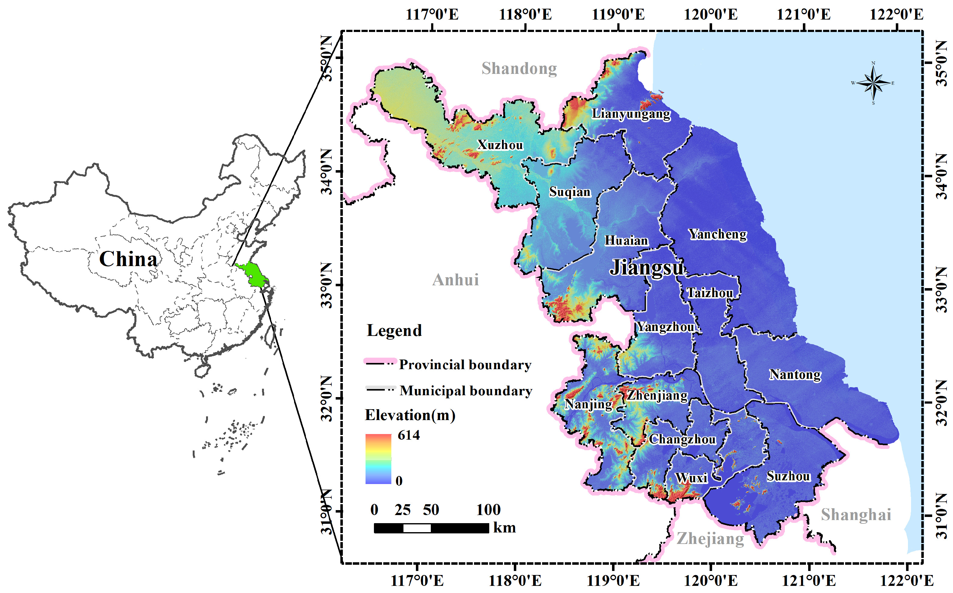
As shown in Figure 1, Jiangsu Province is located in the centre of the eastern coast of Mainland China, spanning a longitude of E to E and a latitude of N to N, in the lower reaches of the Yangtze River and the Huai River, bordering the Yellow Sea to the east, with a coastline of 954 km, bordering Shandong to the north, Anhui to the west, and Shanghai and Zhejiang to the south-east. The inter-provincial land boundary line is 3383 km and covers an area of 107,200 km, accounting for 1.1% of the total area of the country, with the least land area per capita among the Chinese provinces and regions.
With the flat topography and huge plains, Jiangsu is one of the provinces with the lowest terrain in China. The Yangtze River Delta Plain, the Eastern Coastal Plain, the Southern Jiangsu Plain, the Jianghuai Plain, and the Huanghuai Plain make up the majority of the province’s 70,600 km of plains, which dominate the landscape. The province’s low hills are largely found in the Laoshan Mountains, Yuntai Mountains, Ningzhen Mountains, Maoshan Mountains, Yili Mountains, and Huaiyin Mountains, which together make about 14% of the province’s total area [27].
Jiangsu Province is located in the climatic transition zone between the warm-temperate and subtropical zones, with a distinct humid monsoon climate. The weather is mild throughout the region, with abundant rainfall and distinct seasonal changes. The province’s average annual sunshine hours are 2000–2600 h, with a sunshine percentage of 48–59%, with more sunshine hours in summer and less in winter, more in spring than in autumn in Huabei, and more in autumn than in spring in Huainan. The province’s average annual precipitation ranges from 724 to 1210 mm, and the province’s annual evaporation ranges from 900 to 1050 mm, with an obvious trend of increasing evaporation from east to west due to the influence of humid ocean currents [28]. Each region’s average temperature ranges from 13 to 16 C, gradually increasing from north-east to south-west. The province has numerous interconnected rivers and dense water networks. According to statistics from 2017, Jiangsu has 17,300 km of inland water surface area, which accounts for 17% of the province’s total area, making it the province with the highest proportion of water area in the country (according to Jiangsu Statistical Yearbook 2017). The province has over 2900 large and small rivers, 290 lakes, and over 1100 reservoirs. Taihu Lake and Hongze Lake, located in the wet Jiangnan and northern Jiangsu plains, respectively, are two of China’s five largest freshwater lakes.
With a 22.8% of forest coverage in 2016, Jiangsu Province holds 1.56 million hectares of forests. Deciduous broad-leaved forests, mixed evergreen broad-leaved forests, and evergreen broad-leaved forests make up the majority of the many forms of terrestrial vegetation. Wet and aquatic vegetation as well as salt vegetation are examples of non-zonal vegetation.
2.2. Annual Surface PM Product
The study employed an authoritative and publicly available PM product from the Atmospheric Composition Analysis Group of Dalhousie University [29]. The annual surface PM product (version: V4.NA.01) covers 1998 to 2015 with a spatial resolution of 1 km. It is derived from the AOD product calculated with the GEOS-Chem chemical transport model using remote sensing data from NASA MODIS, MISR, and SeaWIFS. In addition, a geographically weighted regression (GWR) model is used to calibrate ground-based PM monitoring data [30]. The PM data of version V4.NA.01 was obtained from the Socioeconomic Data and Applications Center (SEDAC)—hosted by the Center for International Earth Science Information Network (CIESIN) at Columbia University (http://sedac.ciesin.columbia.edu/, accessed on 7 October 2015 ). Due to the provider’s change in employment, a new address (https://sites.wustl.edu/acag/datasets/surface-pm2-5/, accessed on 31 July 2022) is maintained by Washington University in St. Louis [30]. In comparison with the ground-based observation on PM concentrations, related studies have tested the dataset with an accuracy of 0.8 in several Chinese regions [12,31], allowing for its reliable use in Jiangsu. Hence, the PM series data from 2000 to 2015 are selected for the Jiangsu Province in this work.
2.3. Methods
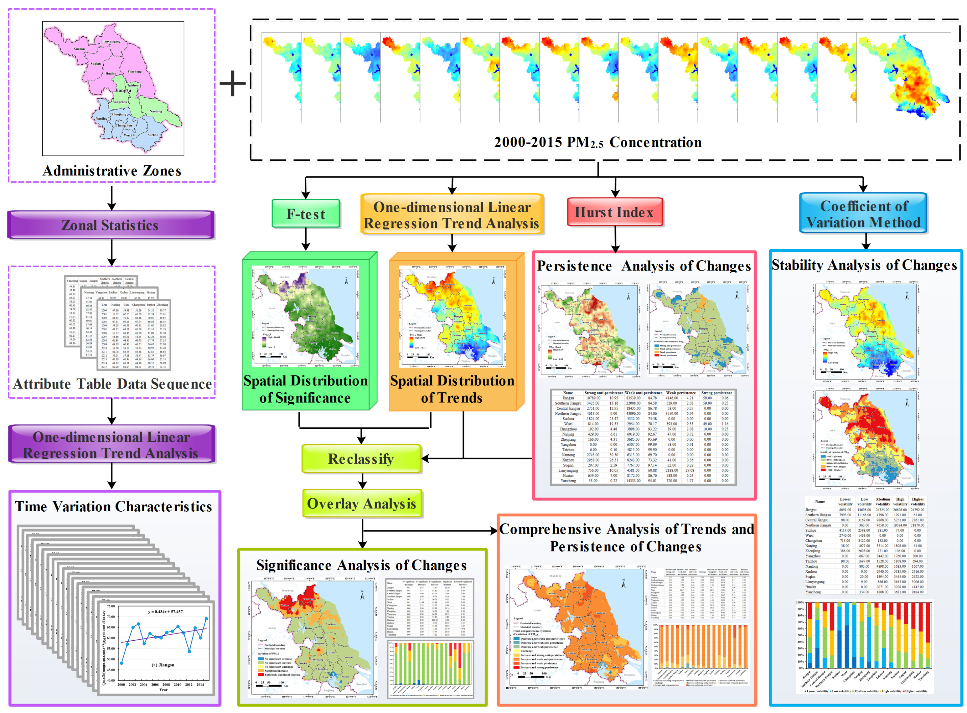
In this study, time series analysis techniques, such as univariate linear regression and the corresponding F-test, coefficient of variation method, and Hurst index, were used to examine the temporal variation characteristics and spatial pattern evolution of PM in Jiangsu Province since 2000. In Figure 2, the detailed methodology is displayed.
The developed methodology comprises three steps: In the beginning, zonal statistics with the vector data of Jiangsu’s administrative divisions were used to determine the yearly average PM concentration for 13 prefecture-level cities, three main subregions, and the entire province. On this premise, the univariate linear regression of the trend analysis was used to reveal the temporal fluctuation of PM concentrations for the above zones. Secondly, trend analysis methods of univariate linear regression were also utilized for pixel-wise trend prediction and the spatio-temporal mapping of trends. Moreover, the F-test were used to examine the confidence of the trend statistical analysis. The variation coefficient, meanwhile, was calculated to quantify the stability characteristics of the PM concentration time series changes. Finally, with the Hurst index, the persistent characteristics of various trends in the time series of PM concentrations were investigated. Combining the current trends, the possibility of trend continuation or reversal in the future can be estimated for PM concentrations. The overall statistical criteria are listed in Table 1 and more details of the methods are given below.
2.3.1. Univariate Linear Regression
In this study, the trend analysis is based on univariate linear regression and is performed directly with time as the independent variable. Trend analysis for the series at each pixel can yield the spatial pattern of a trend, which can directly describe the characteristics of regional changes [12]. As the most straightforward way to estimate trends, the univariate linear regression can effectively remove outliers and avoid interference from additional factors to obtain the dominant trend. The slope of the fitted straight line reflects the overall trend of PM concentrations from 2000 to 2015. It is calculated using Equation (1):
where is the slope of the regression line, n is the number of years within a series, i is the number of years from 1 to 16, and is the PM concentration in year i.
To determine the significance of the estimated trends, the F-test was used. Note that the significance level reflects the level of belief in the trend change and has nothing to do with the rate of change. The formula for calculating this is as follows:
where U is the sum of squares of regression, Q is the sum of squares of error, is the actual observed value of year i, is the predicted value, is the mean value of the 16-year series, and n is the number of years. According to the estimated significance level, these trends can be classified into the following nine classes as listed in Table 2.
2.3.2. Coefficient of Variation
The coefficient of variation is a statistical measure of the variation of a temporal series. It enables to accurately capture the fluctuation characteristics of the PM concentration time series at each pixel. The higher the coefficient of variation, the more discrete the distribution of the PM concentration is, and the inter-annual variation of the concentration is more volatile; conversely, it indicates that the distribution of the PM concentration is concentrated, and the series is regarded as stable. It is calculated using the following formula.
where n is the number of years and C is the PM concentration of the i-th year.
2.3.3. Hurst Index
The Hurst index is frequently described as the “index of dependence” or “index of long-range dependence”. It estimates the relative tendency of a time series to either substantially regress to the mean or to cluster in a certain direction [32]. In other words, it can be considered as a trend inertia. We used the Hurst index to measure the long-term memory of the series, which is related to the autocorrelations of the time series, and the rate at which these decrease as the lag between pairs of values increases. In this paper, the rescaled range (R/S) analysis was used to estimate the Hurst index. The rescaled range analysis examines a data series to determine the persistence or mean-reverting tendencies within that data [33]. For the PM concentration series , the rescaled range was calculated as follows: The time series is first divided into m equal-length subsequences , the length of which is l. The elements of is denoted as , and . Here we assume that the length of the subsequence can be variable, i.e., l can be 2, 4, 8, or 16. Simultaneously, the number of subsequences is set as 8, 4, 2 and 1. For a subsequence , the mean-adjusted subsequence is calculated by
where is the cumulative deviation of the k-th element in the i-th subsequence and is the mean value of . Next, the extreme deviation of the i-th subsequence is given as follows,
is the standard deviation of and the rescaled extreme deviation is defined as all the expected m-rescaled extreme deviations and calculated as,
The varies significantly corresponding to the length l of a subsequence. Finally, the Hurst index H can be estimated using Equation (7),
where K is a constant. The least squares regression of log and log can be used to estimate the H. The Hurst index H indicates the persistence of changes or trends, which includes three cases corresponding to the value of H:
- if 0.5 < H < 1, the time series is considered to be persistent, which means that the characteristics of future changes will be the same as those of past changes. The closer H is to 1, the more visible the persistence is.
- If H is equal to 0.5, the time series is a random series without long-term persistence.
- if 0 < H < 0.5, the time series exhibits inverse persistence, which means that the trends of future change and those of previous change are extremely unlike.
3. Results
3.1. Temporal Variation Characteristics of the PM Concentration
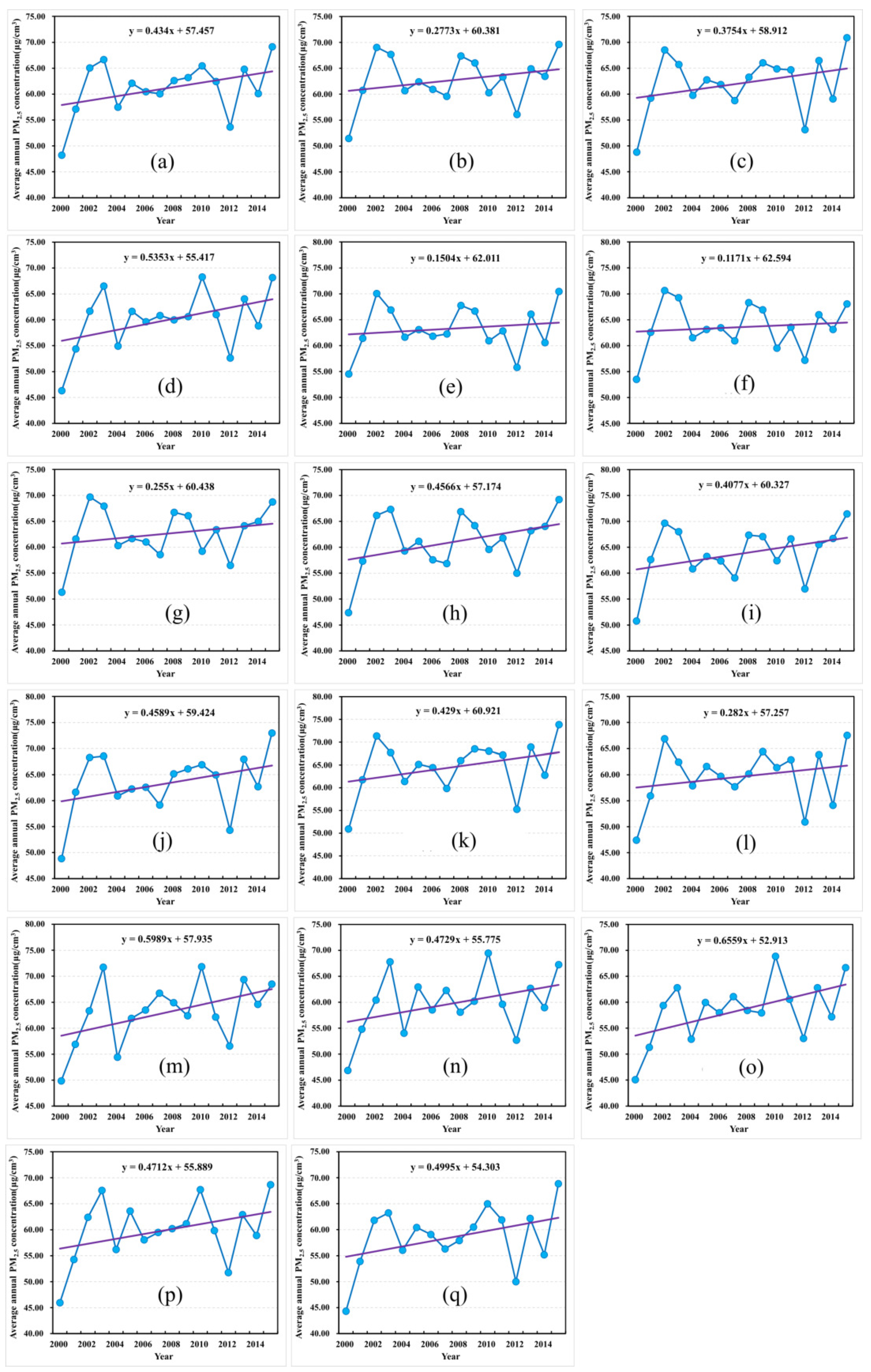
Analysing with univariate linear regression, the estimated trends of the annual average concentrations of PM in the whole province, subregions, and various cities is shown in Figure 3. The province as a whole exhibits an overall oscillating upward trend, increasing at an average rate of 0.434 g/cm, and the PM concentration increased by 0.92 g/cm in 2015 compared to 2000. The PM concentration increased the fastest between 2012 and 2013, with an increase of 11.15 g/cm, accounting for 53.30% of the overall increase. The highest value of 69.61 g/cm was reached in 2015, indicating an overall deterioration in air quality. The three subregions—the southern, the central, and the northern—all exhibit a varying upward trend overall, increasing at rates of 0.2773, 0.3754 and 0.5353 g/cm per year, respectively. The fastest increase was observed in northern Jiangsu, where the PM concentrations in 2015 rose by 18.13, 22.09, and 21.82 g/cm compared to 2000. The three subregions essentially reached the highest values in 2015, with values of 69.61, 70.89, and 68.15 g/cm, respectively. The northern and central regions of Jiangsu showed the fastest increase between 2012 and 2013, with increases of 11.42 and 13.34 g/cm, accounting for 52.34 and 60.38% of the overall increase, respectively. Southern Jiangsu experienced the fastest growth of PM concentrations between 2000 and 2001, with an increase of 9.30 g/cm that accounted for 51.26% of the overall increase. Following that, the PM concentration gradually fluctuated upwards.
Additionally, Figure 3 depicts the change patterns of PM concentrations during the previous 16 years in each prefecture-level city of Jiangsu Province. PM concentrations of each prefecture-level city exhibit a strong rising trend and consistent fluctuations, following a similar trend as the province, while the concentration fluctuations of PM between prefecture-level cities varied most in magnitude and rate and were inconsistent with that of the whole province. Lianyungang, with an increasing rate of 0.6559 g/cm of the PM concentration, had the greatest increase in PM concentration, followed by Xuzhou City in the north. Wuxi and Suzhou, with the highest PM concentration levels in 2000, are generally stable and show the slowest rates of growth. In terms of magnitude variation, the PM concentrations of Yancheng, Huai’an and Lianyungang in northern Jiangsu, Yangzhou and Taizhou in central Jiangsu, and Nanjing in southern Jiangsu all increased by more than 45.00%.
Note that the reduction in PM concentration in each prefecture-level city between 2006 and 2012—particularly in 2012—was primarily brought about by the positive effects of the 11th Five-Year Plan’s “energy conservation and emission reduction” policies and the 12th Five-Year Plan’s “green development, building a resource-saving and environment-friendly society” policies in Mainland China.
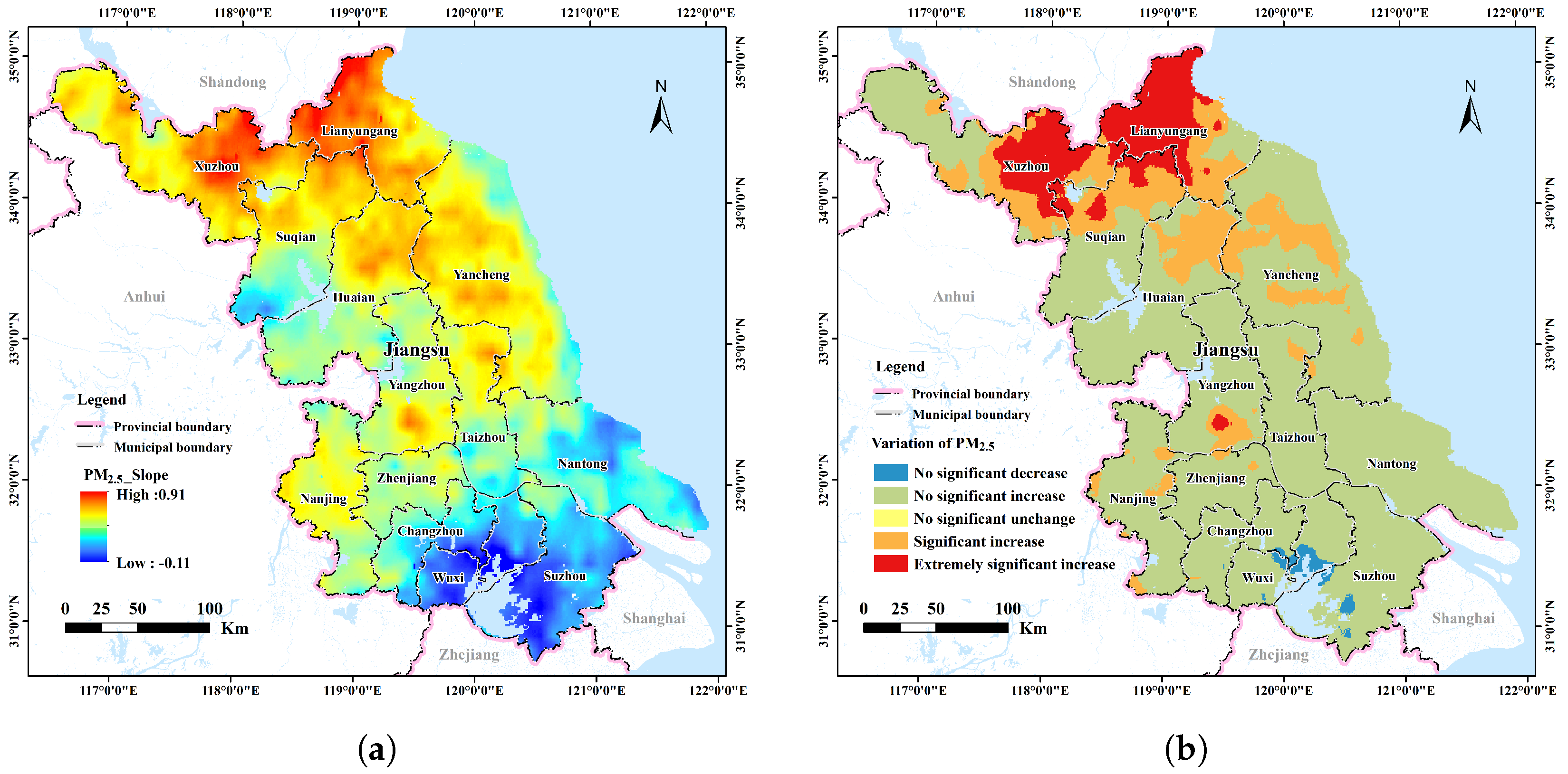
As shown in Figure 4a, the spatial distribution of fitted by regression is given and indicates the pixel-wise trends and change intensity of the PM concentration in Jiangsu Province. The value of varies from −0.11 to 0.91, suggesting that the of the PM concentrations of most areas is greater than zero. To be exact, the proportion of the area with increasing PM concentration accounts for 99.15%. For cities, it is evident that Xuzhou and Lianyungang in northern Jiangsu have the highest slope values of PM concentration growth, indicating a definite trend of air quality deterioration and the quickest increase in concentration. Conversely, the cities around Taihu Lake in southern Jiangsu, such as Wuxi and Suzhou, hold a zero slope value, indicating that the change in PM concentrations in these areas is negligible.
The significance of the change in PM concentration over the entire Jiangsu Province can be divided into nine categories based on the significance level of the F-test. Since three categories account for negligible, only five categories are finally obtained and displayed in Figure 4b. With respect to the growth trends, Yangzhou in the centre of the region and Lianyungang, Xuzhou, and Suqian in the north account for the majority of regions where there is a 24.78% increase at the 90% confidence level and a 9.49% increase at the 95% confidence level. Turned to decreasing trends, the areas where PM decreased accounted for about 0.84% of the total area, mainly distributed in the cities along Taihu Lake. At last, the area of unchanged PM concentrations is extremely small, accounting for only 0.01%.
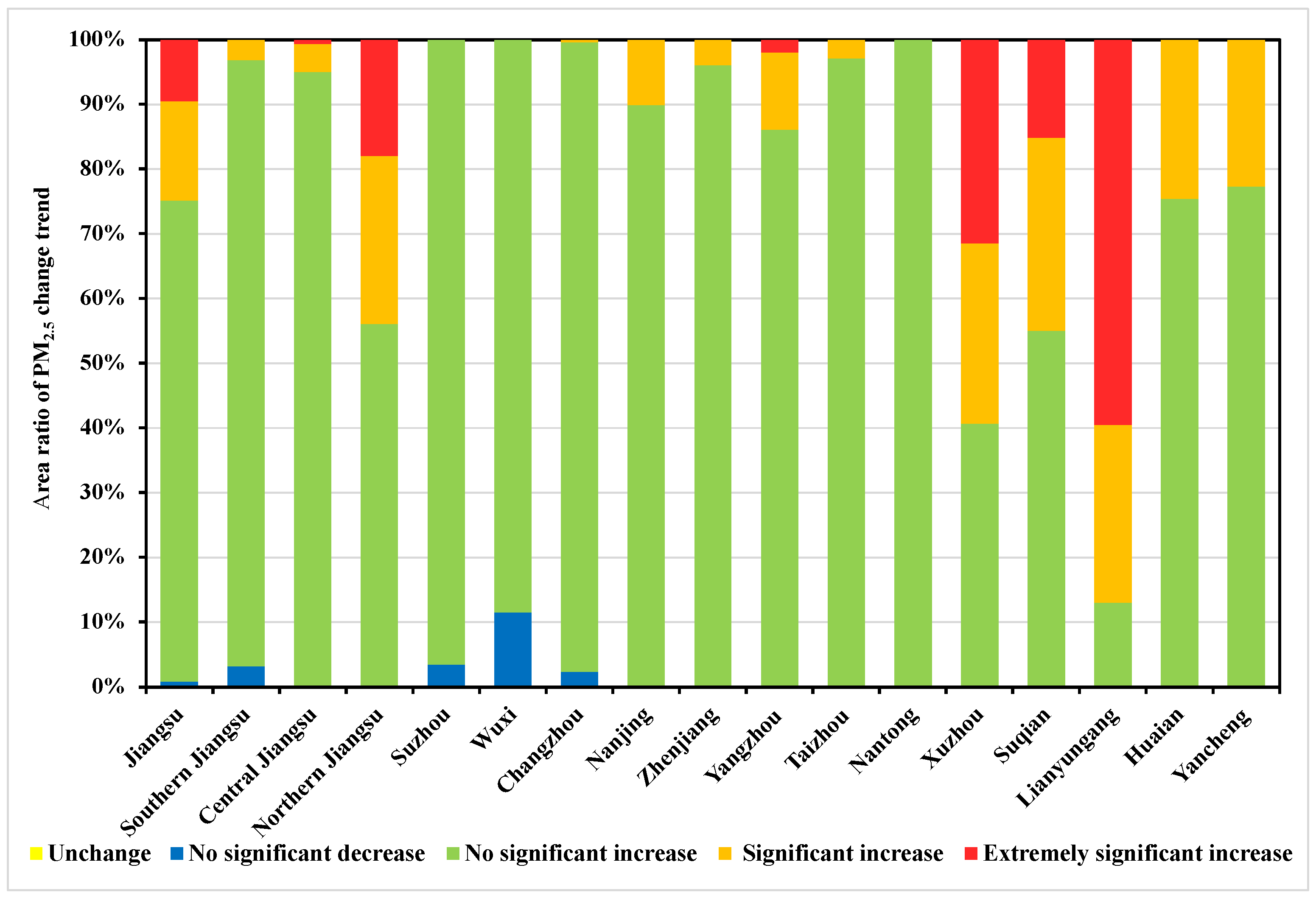
According to Figure 5, the varying trends are typically consistent with those of the entire province, but the varying intensity is inconsistent. In the southern Jiangsu region, all other cities saw a 100% increase in PM concentrations except for Suzhou, Wuxi, and Changzhou. In the northern Jiangsu region, the proportion of Lianyungang exhibited an upward trend of 86.77% at the 95% confidence level and 59.58% at the 90% confidence level. At the 90% confidence level, the percentages of increasing trends in Xuzhou, Suqian, Huaian, Yancheng in northern Jiangsu, Yangzhou and Nanjing in central Jiangsu are 59.27, 44.97, 24.56, 22.68, 13.94 and 10.14%, respectively. The decreasing trends of PM concentrations are aggregated in Suzhou, Wuxi and Changzhou along Taihu Lake in southern Jiangsu Province, with an area of about 825.00 km, only accounting for 0.84% of the total area, and the confidence level is low.
3.2. Stability Analysis of the PM Concentration Changes
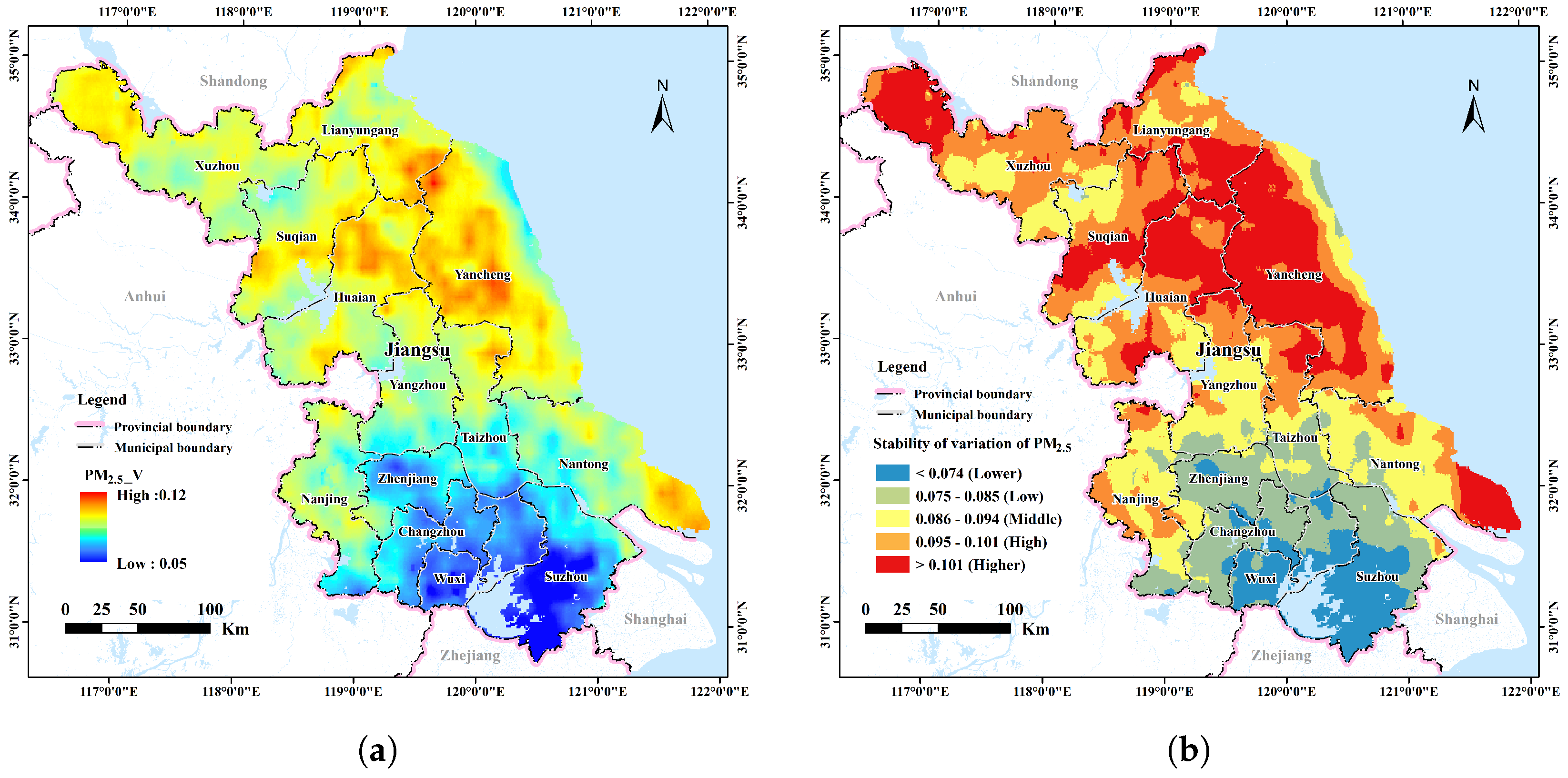
The variability characteristics of the PM concentration series in Jiangsu Province from 2000 to 2015 are obtained using the coefficient of variation method, as shown in Figure 6a. The mapping of variation coefficient V is then reclassified into five classes using the natural breakpoint method, with the results displayed in Figure 6b. Table 3 shows the outcomes of zonal statistics according to three subregions and prefecture-level cities for the stability of PM concentration variations in 13 cities and three subregions in Jiangsu Province.
A general spatial pattern of “high in the north and low in the south” is seen in Jiangsu Province’s coefficient of variation for the PM concentrations from 2000 to 2015, ranging from 0.05 to 0.12. Among them, the area in northern Jiangsu with high volatility is 21.87 million km, accounting for 88.21% of the area in the province; the area in southern Jiangsu with low volatility is 98.79% of the area in the province; and the variability in central Jiangsu is between northern and southern Jiangsu. Accordingly, in Jiangsu Province, the variability of the PM concentration generally decreases from northern to southern Jiangsu, with the least volatility and reasonably consistent inter-annual variability in southern Jiangsu.
There is a distinct spatial pattern of variability inside each prefecture-level city, despite the fact that the overall spatial pattern of the province’s variability is “high in the north and low in the south”. Northern Jiangsu’s high-volatility region accounts for 42.65% of the region, with Yancheng City’s high volatility making up for 60.87% of the city. On the other hand, Huai’an, Lianyungang, Suqian, and Xuzhou City, with 43.97, 39.94, 32.77, and 25.94% of the area, respectively, have the highest volatility. In the central Suzhou region, the cities of Yangzhou, Taizhou, and Nantong account for 54.04, 26.23, and 54.10%, respectively, of the area of moderate volatility. In southern Jiangsu, the cities with most stable changes are Suzhou, Wuxi, Changzhou, Zhenjiang, and Nanjing, with low-volatility zones accounting for 65.19, 57.38, 16.68, 10.02, and 0.58%, respectively.
3.3. Persistence Analysis of the PM Concentration Changes
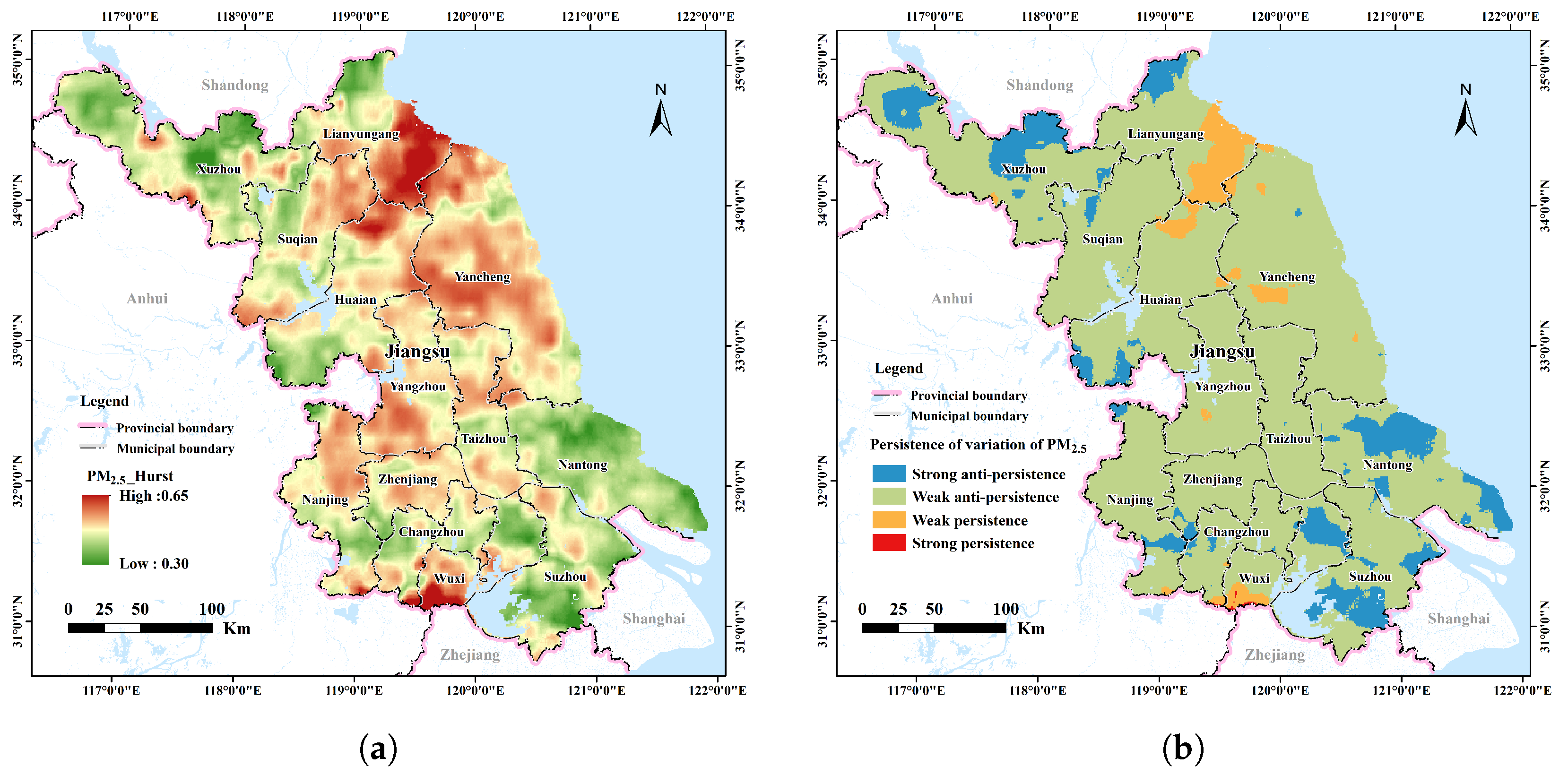
The persistence of the PM concentration fluctuations between 2000 and 2015 over Jiangsu Province is shown in Figure 7a thanks to the Hurst index analysis. Figure 7b illustrates the reclassification of the Hurst index into the four categories: strong inverse persistence (SIP), weak inverse persistence (WIP), weak persistence (WP), and strong persistence (SP). The zonal statistics-derived persistent estimates of the PM concentration changes in the 13 prefecture-level cities and three subregions are presented in Table 4.
In Jiangsu Province, the Hurst index for the persistence estimation of the PM concentration ranges from 0.30 to 0.65, demonstrating a pattern of “reverse persistence dominated by positive persistence”. In total, 4.27% of the whole province presented positive persistence, and 4.21% presented weak positive persistence. On the other hand, 95.73% of the province’s areas exhibited anti-persistence, and 88.56% exhibited weak anti-persistence. With a total size of 3559 km, the areas of weak anti-persistence make up the majority of Jiangsu Province’s northern region, accounting for 85.84% of the positive persistence area of Jiangsu Province. When compared to northern and central Jiangsu, the areas of weak anti-persistence in central Jiangsu obtain the highest percentage at 86.78%, while the areas of strong anti-persistence in southern Jiangsu obtain the highest percentage at 13.16%.
In addition, the spatial distribution of the Hurst index at the city-scale also exhibits significant differences. The largest area of weak positive persistence is found in Lianyungang, covering 2188 km, or 29.08% of its municipal territory. On the other hand, Nantong, Xuzhou, and Suzhou, which account for 30.3, 26.31, and 25.42% of their municipal territory, respectively, are the top three cities with strong anti-persistence. Taizhou, Yangzhou, Suqian, Zhenjiang, Yancheng, Changzhou, and Nanjing are the prefecture-level cities with the area percentage of weak anti-persistence areas higher than 90%, accounting for 99.90, 99.09, 97.14, 95.69, 95.01, 93.22, and 92.67%, respectively.
3.4. Comprehensive Analysis of the Trend and Persistence of PM Concentration Changes
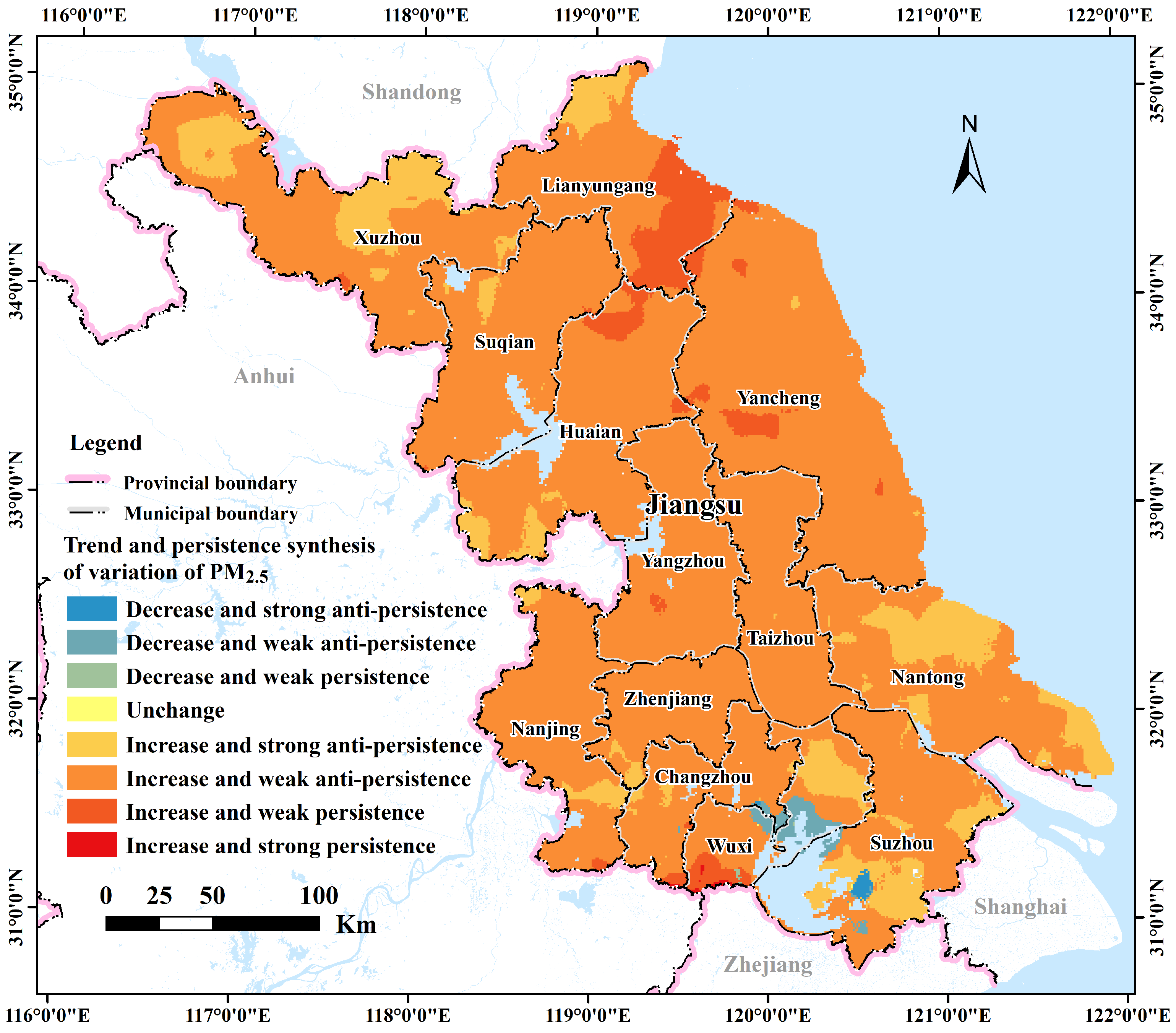
To synthetically analyse the interrelationship between the change trend and persistence and their combination pattern in space. We applied superposition analysis to combine the Hurst index and change trend results to obtain a new spatial pattern, as shown in Figure 8. The figure presents eight spatial combination patterns, including decrease and strong anti-persistence, decrease and weak anti-persistence, decrease and weak positive persistence, increase and strong anti-persistence, increase and weak anti-persistence, increase and weak positive persistence, increase and strong positive persistence, and no change. Furthermore, by using zonal statistical analysis, the trend and persistence of changes in PM concentrations in three subregions and 13 cities in Jiangsu Province are obtained, as shown in Figure 9.
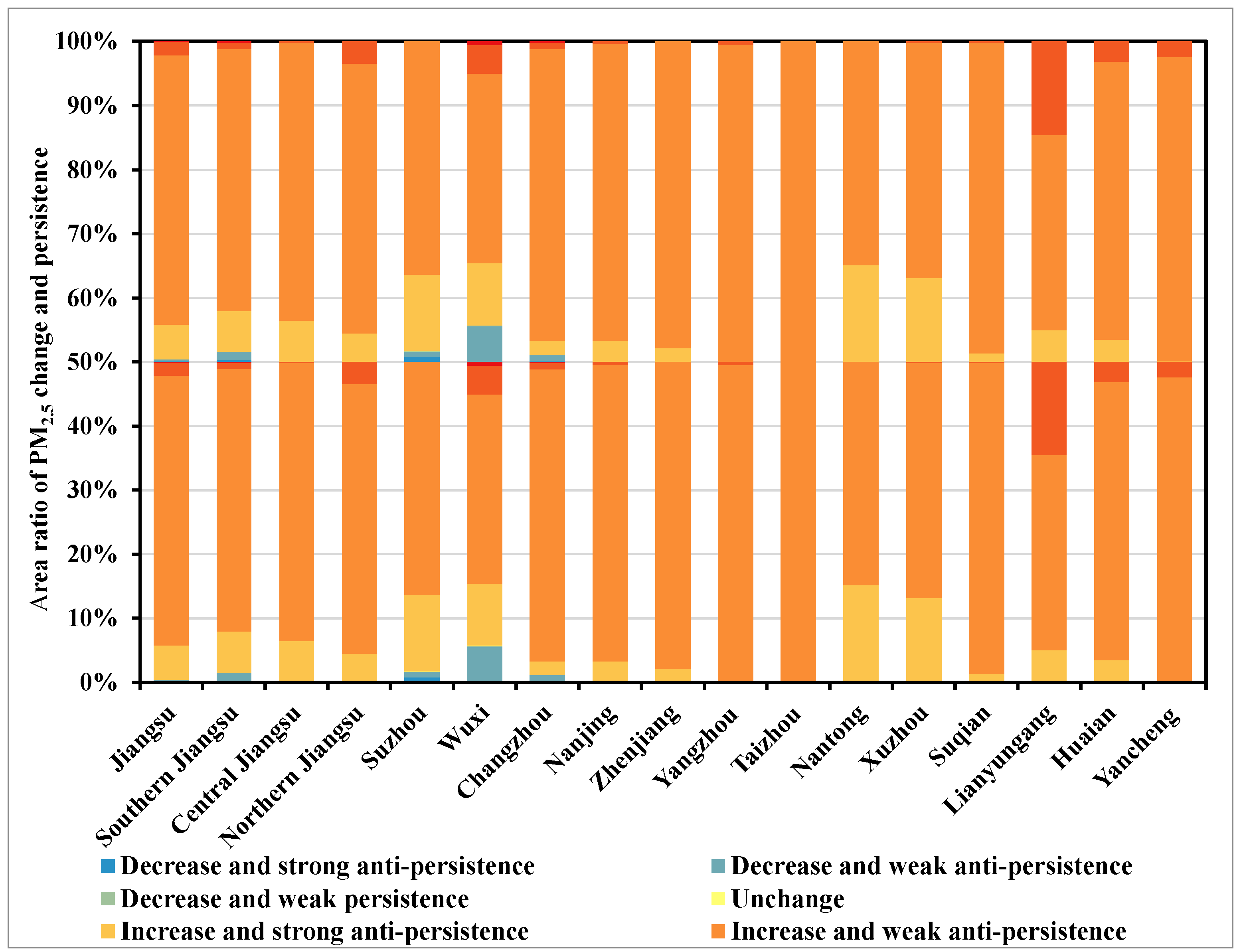
The class of increase with weak anti-persistence, as one of the eight combination types, accounts for 84.09% of the province’s total area. This is followed by the combination class of increase with strong anti-persistence, and increase and weak positive persistence, accounting for 10.82 and 4.19% of the province’s area, respectively. Less than 1% of the area is occupied by the remaining five combination classes. The three combinations—increase and strong anti-persistence, increase and weak anti-persistence, and increase and weak positive persistence—are scattered over northern and central Jiangsu. Moreover, the corresponding three categories made up 9, 84.06, and 6.94%, respectively, in northern Jiangsu.
With respect to the individual cities, each city indicates a unique combination of trend and persistence patterns. The decrease and strong anti-persistence category is primarily designated to Suzhou and Changzhou. The Suzhou–Wuxi–Changzhou metropolitan area is designated with the decrease and weak anti-persistence category. Note that only Wuxi is designated with the decrease and weak positive persistence category. The remaining 12 prefecture-level cities, except for Yangzhou, are designated with the increase and strong anti-persistence category. The top three by area proportion are Nantong, Xuzhou, and Suzhou with percentages od 30.30, 26.31, and 23.72%, respectively. The predominant class in each city is the increase and weak anti-persistence class, and the top three by area proportion are Taizhou, Yangzhou, and Suqian City, with percentages of 99.90, 99.09, and 97.12%, respectively. The class of increase and weak positive persistence is mainly designated in Lianyungang, Wuxi and Huai’an, with an area share of 29.07, 8.93 and 6.24%, respectively. Note that with an area proportion of almost 0, the class of increase and strong persistence and the unchanged class are only distributed in Wuxi, Changzhou and Suzhou.
4. Discussion
Compared with similar studies in China, our work focuses more on the intensity of temporal variation as well as persistence or inertia than trends in change. In addition, smaller geographical scales are considered corresponding to the spatial variability of the underlying surface. Although some scholars at the same scale have carried out the analysis of spatio-temporal patterns for prefecture-level cities in southern Jiangsu, Shandong, Anhui, Beijing–Tianjin–Hebei and the whole of China, only the studies with ground-based PM concentrations over Shandong and Beijing–Tianjin–Hebei region introduced the concept of convergence or a relationship between pollution intensity and space–time variation to characterize the inertia of change [22,23]. From a data perspective, our study analyses the characteristics of temporal variation at a higher granularity using satellite-derived PM products, while the results demonstrate that such temporal characteristics vary with respect to spatial variability of the underlying surface. This will further inspire subsequent studies on the interaction between the underlying surface and temporal variation patterns.
Limited by the spatial and temporal resolution of the PM data, our study only analyses the inter-annual variability characteristics and cannot further explain the influence of seasonal climate on the temporal phase variability characteristics. In the near future, multi-timescale investigations of the local underlying surface on the spatio-temporal variability of PM concentrations will soon exploit these local time-varying properties with the availability of higher-spatial-resolution PM products.
5. Conclusions
In this paper, we focus on the time series analysis of PM concentrations in Jiangsu Province from 2000 to 2015. The spatio-temporal patterns of trends, stability and persistence are mapped and analysed with the methods of univariate linear regression, coefficient of variation estimation and Hurst index estimation. The main conclusions are as follows:
(1) The increasing trends or slopes of PM in Jiangsu Province are not consistent at the prefecture-level, but they are consistent in northern, central and southern Jiangsu at a larger scale. In detail, the overall pattern is that the PM concentration growing rate decreases from north to south. In particular, Xuzhou and Lianyungang have significantly more serious PM air pollution than other regions and the fastest rising concentrations. In contrast, the urbanization level of cities around Taihu Lake was already higher than in the north in 2000, as well as the PM air pollution. Thus, PM concentrations of these lakeside cities began at a high level and and increase at a slow rate. This suggests that the intensity of urbanization activities is one potential cause for the increase in PM air pollution.The outcomes of the trend analysis and significance test reveal that Jiangsu Province’s overall PM pollution has been rising since 2000. Cities in the province, however, have varying air pollution levels and rates of rise in PM. In detail, the overall pattern is that the PM concentration growth rate decreases from north to south. In particular, Xuzhou and Lianyungang have significantly more serious PM air pollution than other regions and the fastest rising concentrations. In contrast, the urbanization level of cities around Taihu Lake was already higher than in the north in 2000, as well as PM air pollution is. Thus, PM concentrations of these lakeside cities starting from a high level and increasing at a slow rate. This suggests that the intensity of urbanization activities is one of the potential causes of the increase in PM air pollution.
(2) The spatial pattern of temporal variability of PM concentrations in Jiangsu generally shows a decreasing pattern from north to south. The areas with variability from medium to high levels are mainly aggregated in areas north of the Yangtze River. Yancheng has the highest degree of fluctuation, followed by Huai’an and Lianyungang, while Suzhou and Wuxi have the most stable variability of PM concentrations, with a strong inertia to external disturbance factors.
(3) Combining the results of the persistence analysis and trend analysis, it can be found that the pattern of the combination of increase and weak anti-persistence accounts for most of Jiangsu, while the area of the strong persistence region is the least, indicating that PM air pollution in Jiangsu Province may develop in a good direction in the future, i.e., there is a possibility of it slowing down the deteriorating trend of air quality in the future. However, the combined pattern of increase and weak positive persistence exists in Lianyungang, Yancheng and Wuxi, and thus, the PM air pollution in these areas will maintain the deterioration trend.
Author Contributions
Conceptualization, J.L.; methodology, J.L.; software, J.L.; validation, J.L., and M.C.; formal analysis, J.L.; investigation, J.L.; resources, J.L.; data curation, J.L.; writing—original draft preparation, M.C.; writing—review and editing, J.L. and M.C.; visualization, J.L.; supervision, M.C.; project administration, J.L.; funding acquisition, J.L. All authors have read and agreed to the published version of the manuscript.
Funding
This research was funded by the National Natural Science Foundation of China (Grant No. 42001239 and No. 62201295), the Basic Science Research Program of Nantong(Grant No. JC12022101).
Institutional Review Board Statement
Not applicable.
Informed Consent Statement
Not applicable.
Data Availability Statement
The data are available from the corresponding authors by request.
Acknowledgments
The authors would like to thank the Atmospheric Composition Analysis Group of Dalhousie University for providing the PM product data.
Conflicts of Interest
The authors declare no conflict of interest.
References
- Englert, N. Fine particles and human health—A review of epidemiological studies. Toxicol. Lett. 2004, 149, 235–242. [Google Scholar] [CrossRef]
- Ma, Z.; Dey, S.; Christopher, S.; Liu, R.; Bi, J.; Balyan, P.; Liu, Y. A review of statistical methods used for developing large-scale and long-term PM2. 5 models from satellite data. Remote Sens. Environ. 2022, 269, 112827. [Google Scholar] [CrossRef]
- Wang, Q.; Kwan, M.P.; Zhou, K.; Fan, J.; Wang, Y.; Zhan, D. The impacts of urbanization on fine particulate matter (PM2.5) concentrations: Empirical evidence from 135 countries worldwide. Environ. Pollut. 2019, 247, 989–998. [Google Scholar] [CrossRef]
- Guo, H.; Cheng, T.; Gu, X.; Wang, Y.; Chen, H.; Bao, F.; Shi, S.; Xu, B.; Wang, W.; Zuo, X.; et al. Assessment of PM2.5 concentrations and exposure throughout China using ground observations. Sci. Total Environ. 2017, 601, 1024–1030. [Google Scholar] [CrossRef]
- Zhang, W.; Zheng, F.; Zhang, W.; Yang, X. Estimating Ground-Level Hourly PM2.5 Concentrations Over North China Plain with Deep Neural Networks. J. Indian Soc. Remote Sens. 2021, 49, 1839–1852. [Google Scholar] [CrossRef]
- Xing, Q.; Sun, M. Characteristics of PM2. 5 and PM10 Spatio-Temporal Distribution and Influencing Meteorological Conditions in Beijing. Atmosphere 2022, 13, 1120. [Google Scholar] [CrossRef]
- Chu, H.J.; Huang, B.; Lin, C.Y. Modeling the spatio-temporal heterogeneity in the PM10–PM2.5 relationship. Atmos. Environ. 2015, 102, 176–182. [Google Scholar] [CrossRef]
- Zhang, A.; Qi, Q.; Jiang, L.; Zhou, F.; Wang, J. Population exposure to PM2.5 in the urban area of Beijing. PLoS ONE 2013, 8, e63486. [Google Scholar] [CrossRef]
- Ma, Z.; Hu, X.; Huang, L.; Bi, J.; Liu, Y. Estimating ground-level PM2.5 in China using satellite remote sensing. Environ. Sci. Technol. 2014, 48, 7436–7444. [Google Scholar] [CrossRef]
- Van Donkelaar, A.; Martin, R.V.; Brauer, M.; Boys, B.L. Use of satellite observations for long-term exposure assessment of global concentrations of fine particulate matter. Environ. Health Perspect. 2015, 123, 135–143. [Google Scholar] [CrossRef]
- Xie, R.; Sabel, C.E.; Lu, X.; Zhu, W.; Kan, H.; Nielsen, C.P.; Wang, H. Long-term trend and spatial pattern of PM2.5 induced premature mortality in China. Environ. Int. 2016, 97, 180–186. [Google Scholar] [CrossRef] [PubMed]
- Peng, J.; Chen, S.; Lü, H.; Liu, Y.; Wu, J. Spatiotemporal patterns of remotely sensed PM2.5 concentration in China from 1999 to 2011. Remote Sens. Environ. 2016, 174, 109–121. [Google Scholar] [CrossRef]
- Ouyang, X.; Wei, X.; Li, Y.; Wang, X.C.; Klemeš, J.J. Impacts of urban land morphology on PM2.5 concentration in the urban agglomerations of China. J. Environ. Manag. 2021, 283, 112000. [Google Scholar] [CrossRef] [PubMed]
- Wang, X.; Li, T.; Ikhumhen, H.O.; Sá, R.M. Spatio-temporal variability and persistence of PM2.5 concentrations in China using trend analysis methods and Hurst exponent. Atmos. Pollut. Res. 2022, 13, 101274. [Google Scholar] [CrossRef]
- Crippa, M.; Janssens-Maenhout, G.; Guizzardi, D.; Van Dingenen, R.; Dentener, F. Contribution and uncertainty of sectorial and regional emissions to regional and global PM2.5 health impacts. Atmos. Chem. Phys. 2019, 19, 5165–5186. [Google Scholar] [CrossRef]
- Zhang, L.; Wilson, J.P.; MacDonald, B.; Zhang, W.; Yu, T. The changing PM2.5 dynamics of global megacities based on long-term remotely sensed observations. Environ. Int. 2020, 142, 105862. [Google Scholar] [CrossRef]
- Xue, T.; Zheng, Y.; Geng, G.; Zheng, B.; Jiang, X.; Zhang, Q.; He, K. Fusing observational, satellite remote sensing and air quality model simulated data to estimate spatiotemporal variations of PM2.5 exposure in China. Remote Sens. 2017, 9, 221. [Google Scholar] [CrossRef]
- Wei, J.; Li, Z.; Lyapustin, A.; Sun, L.; Peng, Y.; Xue, W.; Su, T.; Cribb, M. Reconstructing 1-km-resolution high-quality PM2.5 data records from 2000 to 2018 in China: Spatiotemporal variations and policy implications. Remote Sens. Environ. 2021, 252, 112136. [Google Scholar] [CrossRef]
- Huang, R.J.; Zhang, Y.; Bozzetti, C.; Ho, K.F.; Cao, J.J.; Han, Y.; Daellenbach, K.R.; Slowik, J.G.; Platt, S.M.; Canonaco, F.; et al. High secondary aerosol contribution to particulate pollution during haze events in China. Nature 2014, 514, 218–222. [Google Scholar] [CrossRef]
- Yang, Y.; Christakos, G.; Yang, X.; He, J. Spatiotemporal characterization and mapping of PM2.5 concentrations in southern Jiangsu Province, China. Environ. Pollut. 2018, 234, 794–803. [Google Scholar] [CrossRef]
- Zhang, H.; Nie, Y.; Deng, Q.; Liu, Y.; Lyu, Q.; Zhang, B. Spatio-Temporal Changes in Air Quality of the Urban Area of Chongqing from 2015 to 2021 Based on a Missing-Data-Filled Dataset. Atmosphere 2022, 13, 1473. [Google Scholar] [CrossRef]
- Yang, Y.; Christakos, G. Spatiotemporal characterization of ambient PM2.5 concentrations in Shandong province (China). Environ. Sci. Technol. 2015, 49, 13431–13438. [Google Scholar] [CrossRef]
- Jiang, L.; He, S.; Zhou, H. Spatio-temporal characteristics and convergence trends of PM2.5 pollution: A case study of cities of air pollution transmission channel in Beijing–Tianjin–Hebei region, China. J. Clean. Prod. 2020, 256, 120631. [Google Scholar] [CrossRef]
- Jia, L.; Sun, J.; Fu, Y. Spatiotemporal variation and influencing factors of air pollution in Anhui Province. Heliyon 2023, 9, e15691. [Google Scholar] [CrossRef]
- Zhou, X.; Zhang, X.; Wang, Y.; Chen, W.; Li, Q. Spatio-temporal variations and socio-economic drivers of air pollution: Evidence from 332 Chinese prefecture-level cities. Atmos. Pollut. Res. 2023, 14, 101782. [Google Scholar] [CrossRef]
- Alyousifi, Y.; Othman, M.; Husin, A.; Rathnayake, U. A new hybrid fuzzy time series model with an application to predict PM10 concentration. Ecotoxicol. Environ. Saf. 2021, 227, 112875. [Google Scholar] [CrossRef]
- Wikipedia Contributors. Jiangsu—Wikipedia, The Free Encyclopedia. 2023. Available online: https://en.wikipedia.org/wiki/Jiangsu (accessed on 3 February 2023).
- Bao, Y.; Meng, C.; Hen, S.; Qiu, X.; Gao, P.; Liu, C. Temporal and Spatial Patterns of Droughts for Recent 50 Years in Jiangsu Based on Meteorological Drought Composite Index. Acta Geogr. Sin. 2011, 66, 599. [Google Scholar] [CrossRef]
- Van Donkelaar, A.; Martin, R.V.; Spurr, R.J.; Burnett, R.T. High-resolution satellite-derived PM2.5 from optimal estimation and geographically weighted regression over North America. Environ. Sci. Technol. 2015, 49, 10482–10491. [Google Scholar] [CrossRef]
- Van Donkelaar, A.; Hammer, M.S.; Bindle, L.; Brauer, M.; Brook, J.R.; Garay, M.J.; Hsu, N.C.; Kalashnikova, O.V.; Kahn, R.A.; Lee, C.; et al. Monthly global estimates of fine particulate matter and their uncertainty. Environ. Sci. Technol. 2021, 55, 15287–15300. [Google Scholar] [CrossRef]
- Luo, J.; Du, P.; Samat, A.; Xia, J.; Che, M.; Xue, Z. Spatiotemporal pattern of PM2.5 concentrations in mainland China and analysis of its influencing factors using geographically weighted regression. Sci. Rep. 2017, 7, 40607. [Google Scholar] [CrossRef]
- Kleinow, T. Testing Continuous Time Models in Financial Markets. Ph.D. Thesis, Humboldt-Universitat, Berlin, Germany, 2002. [Google Scholar]
- Bassingthwaighte, J.B.; Raymond, G.M. Evaluating rescaled range analysis for time series. Ann. Biomed. Eng. 1994, 22, 432–444. [Google Scholar] [CrossRef] [PubMed]
Figure 1.
Location of the study area with topographical information.

Figure 2.
Technical workflow.

Figure 3.
The estimated trends in annual PM concentrations over various cities and subregions of the Jiangsu Province from 2000 to 2015. (a) Jiangsu; (b) Southern Jiangsu; (c) Central Jiangsu; (d) Northern Jiangsu; (e) Suzhou; (f) Wuxi; (g) Changzhou; (h) Nanjing; (i) Zhenjiang; (j) Yangzhou; (k) Taizhou; (l) Nantong; (m) Xuzhou; (n) Suqian; (o) Lianyungang; (p) Huaian; (q) Yancheng.

Figure 4.
The spatial distribution maps of PM change trends and corresponding significance levels for Jiangsu Province. (a) Slope value; (b) significance change.
Figure 4.
The spatial distribution maps of PM change trends and corresponding significance levels for Jiangsu Province. (a) Slope value; (b) significance change.

Figure 5.
A statistical bar chart of the area proportions of five trends over different cities in Jiangsu.
Figure 5.
A statistical bar chart of the area proportions of five trends over different cities in Jiangsu.

Figure 6.
Spatial distribution of variation coefficient of PM change from 2000 to 2015. (a) V value; (b) V class.
Figure 6.
Spatial distribution of variation coefficient of PM change from 2000 to 2015. (a) V value; (b) V class.

Figure 7.
Spatial distribution of the Hurst index of the PM change from 2000 to 2015 in Jiangsu Province. (a) Hurst index; (b) Hurst class.
Figure 7.
Spatial distribution of the Hurst index of the PM change from 2000 to 2015 in Jiangsu Province. (a) Hurst index; (b) Hurst class.

Figure 8.
The spatial mapping of change characteristics for PM concentrations based on the Slope value and Hurst index.
Figure 8.
The spatial mapping of change characteristics for PM concentrations based on the Slope value and Hurst index.

Figure 9.
The area proportions of six classes of change within each city as indicated by the Slope value and Hurst index. Blue color refers to the class of decrease and strong anti-persistence; skyblue color refers to the class of decrease and weak anti-persistence; green color refers to the class of decrease and weak persistence; yellow color refers to the unchanged class; gold color refers to the class of decrease and weak persistence; orange color refers to the class of increase and weak anti-persistence.


Table 1.
Statistical criteria for analysing the temporal characteristics.
| Statistical Methods | Criteria | Input | Description |
|---|---|---|---|
| Linear Regression | The slope of the regression line to indicate the trend of variation. | ||
| F | F-test to determine the significance of the estimated trends. | ||
| Variation coefficient | V | The coefficient to measure variability of the series. | |
| Hurst Index | The i-th element of equal-length subsequences from | ||
| The cumulative deviation of the k-th element in the i-th subsequence in | |||
| The extreme deviation of . | |||
| The standard deviation of . | |||
| The rescaled extreme deviation from the expected rescaled extreme deviations of . | |||
| H | The index to indicate the persistence for variation or trends. |
Table 2.
Temporal trend description of PM variation in nine classesaccording to p value.
| Trend Description | Criteria |
|---|---|
| Highly significant decrease | , or |
| Significant decrease | , or |
| Insignificant decrease | , or |
| Highly significant constant | , or |
| Significant constant | , or or |
| Insignificant constant | , or |
| Insignificant increase | , or |
| Significant increase | , or |
| Highly significant increase | , or |
Table 3.
Statistical results of the area of PM change trend simulated from 2000 to 2015.
| Region | Lowest | Lower | Med | Higher | Highest |
|---|---|---|---|---|---|
| Jiangsu | 8091 | 14,698 | 24,325 | 26,626 | 24,792 |
| Southern Jiangsu | 7993 | 11,166 | 4798 | 1991 | 61 |
| Central Jiangsu | 98 | 3169 | 9868 | 5251 | 2861 |
| Northern Jiangsu | 0 | 363 | 9659 | 19,384 | 21,870 |
| Suzhou | 4114 | 2598 | 381 | 77 | 0 |
| Wuxi | 2740 | 1463 | 0 | 0 | 0 |
| Changzhou | 715 | 3420 | 152 | 0 | 0 |
| Nanjing | 38 | 1077 | 3514 | 1808 | 61 |
| Zhenjiang | 386 | 2608 | 751 | 106 | 0 |
| Yangzhou | 0 | 667 | 3442 | 1760 | 500 |
| Taizhou | 98 | 1697 | 1528 | 1808 | 694 |
| Nantong | 0 | 805 | 4898 | 1683 | 1667 |
| Xuzhou | 0 | 0 | 2940 | 5385 | 2916 |
| Suqian | 0 | 20 | 1894 | 3465 | 2622 |
| Lianyungang | 0 | 9 | 866 | 3645 | 3006 |
| Huaian | 0 | 0 | 2071 | 3208 | 4142 |
| Yancheng | 0 | 334 | 1888 | 3681 | 9184 |
Table 4.
Spatial distribution of the Hurst index of the PM change from 2000 to 2015 in Jiangsu Province.
Table 4.
Spatial distribution of the Hurst index of the PM change from 2000 to 2015 in Jiangsu Province.
| Zone | SIP | WIP | WP | SP | ||||
|---|---|---|---|---|---|---|---|---|
| Area | Percent | Area | Percent | Area | Percent | Area | Percent | |
| Jiangsu | 10,789 | 10.95 | 83,539 | 84.78 | 4146 | 4.21 | 59 | 0.06 |
| Southern Jiangsu | 3425 | 13.16 | 22,008 | 84.58 | 529 | 2.03 | 59 | 0.23 |
| Central Jiangsu | 2751 | 12.95 | 18,435 | 86.78 | 58 | 0.27 | 0 | 0 |
| Northern Jiangsu | 4613 | 9 | 43,096 | 84.06 | 3559 | 6.94 | 0 | 0 |
| Suzhou | 1824 | 25.42 | 5352 | 74.58 | 0 | 0 | 0 | 0 |
| Wuxi | 814 | 19.33 | 2954 | 70.17 | 393 | 9.33 | 49 | 1.16 |
| Changzhou | 192 | 4.48 | 3998 | 93.22 | 89 | 2.08 | 10 | 0.23 |
| Nanjing | 429 | 6.61 | 6019 | 92.67 | 47 | 0.72 | 0 | 0 |
| Zhenjiang | 166 | 4.31 | 3685 | 95.69 | 0 | 0 | 0 | 0 |
| Yangzhou | 0 | 0 | 6307 | 99.09 | 58 | 0.91 | 0 | 0 |
| Taizhou | 6 | 0.1 | 5815 | 99.9 | 0 | 0 | 0 | 0 |
| Nantong | 2745 | 30.3 | 6313 | 69.7 | 0 | 0 | 0 | 0 |
| Xuzhou | 2958 | 26.31 | 8243 | 73.32 | 41 | 0.36 | 0 | 0 |
| Suqian | 207 | 2.59 | 7767 | 97.14 | 22 | 0.28 | 0 | 0 |
| Lianyungang | 756 | 10.05 | 4581 | 60.88 | 2188 | 29.08 | 0 | 0 |
| Huaian | 659 | 7 | 8172 | 86.76 | 588 | 6.24 | 0 | 0 |
| Yancheng | 33 | 0.22 | 14,333 | 95.01 | 720 | 4.77 | 0 | 0 |
Disclaimer/Publisher’s Note: The statements, opinions and data contained in all publications are solely those of the individual author(s) and contributor(s) and not of MDPI and/or the editor(s). MDPI and/or the editor(s) disclaim responsibility for any injury to people or property resulting from any ideas, methods, instructions or products referred to in the content. |
© 2023 by the authors. Licensee MDPI, Basel, Switzerland. This article is an open access article distributed under the terms and conditions of the Creative Commons Attribution (CC BY) license (https://creativecommons.org/licenses/by/4.0/).
Share and Cite
MDPI and ACS Style
Luo, J.; Che, M. Spatio-Temporal Change Pattern Investigation of PM2.5 in Jiangsu Province with MODIS Time Series Products. Atmosphere 2023, 14, 943. https://doi.org/10.3390/atmos14060943
AMA Style
Luo J, Che M. Spatio-Temporal Change Pattern Investigation of PM2.5 in Jiangsu Province with MODIS Time Series Products. Atmosphere. 2023; 14(6):943. https://doi.org/10.3390/atmos14060943
Chicago/Turabian StyleLuo, Jieqiong, and Meiqin Che. 2023. "Spatio-Temporal Change Pattern Investigation of PM2.5 in Jiangsu Province with MODIS Time Series Products" Atmosphere 14, no. 6: 943. https://doi.org/10.3390/atmos14060943
Note that from the first issue of 2016, this journal uses article numbers instead of page numbers. See further details here.