

Inverse Modeling of Formaldehyde Emissions and Assessment of Associated Cumulative Ambient Air Exposures at Fine Scale
Michigan Department of Environment, Great Lakes, and Energy, Lansing, MI 48909, USA
Atmosphere 2023, 14(6), 931; https://doi.org/10.3390/atmos14060931
Submission received: 27 March 2023
/
Revised: 12 May 2023
/
Accepted: 24 May 2023
/
Published: 26 May 2023
(This article belongs to the Special Issue The Michigan-Ontario Ozone Source Experiment (MOOSE))
Abstract
:Among air toxics, formaldehyde (HCHO) is an important contributor to urban cancer risk. Emissions of HCHO in the United States are systematically under-reported and may enhance atmospheric ozone and particulate matter, intensifying their impacts on human health. During the 2021 Michigan-Ontario Ozone Source Experiment (MOOSE), mobile real-time (~1 s frequency) measurements of ozone, nitrogen oxides, and organic compounds were conducted in an industrialized area in metropolitan Detroit. The measured concentrations were used to infer ground-level and elevated emissions of HCHO, CO, and NO from multiple sources at a fine scale (400 m horizontal resolution) based on the 4D variational data assimilation technique and the MicroFACT air quality model. Cumulative exposure to HCHO from multiple sources of both primary (directly emitted) and secondary (atmospherically formed) HCHO was then simulated assuming emissions inferred from inverse modeling. Model-inferred HCHO emissions from larger industrial facilities were greater than 1 US ton per year while corresponding emission ratios of HCHO to CO in combustion sources were roughly 2 to 5%. Moreover, simulated ambient HCHO concentrations depended significantly on wind direction relative to the largest sources. The model helped to explain the observed HCHO concentration gradient between monitoring stations at Dearborn and River Rouge in 2021.
1. Introduction
Formaldehyde (HCHO) is an important Hazardous Air Pollutant (HAP) contributing to cancer risk in the United States (US) [1]. In addition, HCHO exposure can cause eye and airway irritation, allergies, and pulmonary disease [2]. The US Environmental Protection Agency (USEPA, Washington, DC, USA) is proposing to update its HCHO inhalation unit risk (IUR) to 6.4 × 10⁻⁶ (μg/m3)−1 so that a long-term average ambient air concentration of about 1.3 parts per billion by volume (ppb) would correspond to a cancer risk of 1-in-105 [3]. Moreover, the USEPA considers a reference concentration (RfC) of 7 μg/m3, about 5.6 ppb, as a threshold for non-cancer health impacts [3].
The cumulative impacts of ambient HCHO on human health are difficult to assess. On the one hand, cumulative exposure to HCHO alone is the result of both direct emissions (primary HCHO) and chemical formation in the air (secondary HCHO), so a large variety of organic compounds from a multitude of stationary and mobile anthropogenic sources, as well as vegetation (biogenic sources), contributes to ambient concentrations of HCHO. On the other hand, the health impacts of ambient HCHO are exacerbated by reactive chemistry in the air, which enhances the concentrations of ozone and fine particulate matter (PM2.5) due to the atmospheric radicals produced by HCHO decomposition [4,5]. Thus, mitigating HCHO exposure may have multiple air quality co-benefits.
In a previous paper, Olaguer et al. [6] surveyed the scientific literature on regional models of atmospheric HCHO. They also conducted new 1.3 km horizontal resolution modeling of the Southeast Michigan (SEMI) ozone nonattainment area in the US. They noted how current emissions inventories systematically underestimate primary HCHO so that regional air quality models severely underpredict ambient HCHO relative to observations in industrialized cities such as Detroit, Michigan. Citing measurements of ambient HCHO during the 2021 Michigan-Ontario Ozone Source Experiment (MOOSE) [7], Olaguer et al. [6] further demonstrated that the urban HCHO deficit could not be explained by inadequate mechanisms for secondary formation associated with biogenically emitted isoprene, as had been proposed by Marvin et al. [8].
The University of Michigan School of Public Health (UMSPH) [9] recently reviewed the status and long-term trends of ambient HCHO exposure in metropolitan Detroit based on 20 years of monitoring data at three regulatory stations (Dearborn, Southwest Detroit, River Rouge) within 5 km of each other in a heavily industrialized section of SEMI. Long-term average concentrations were 2.2 ppb for Southwest Detroit, 2.6 ppb for Dearborn, and 3.2 ppb for River Rouge. The highest level (River Rouge) corresponded to the 84th percentile of all ground-level HCHO measurements in the US over the same period, while the lowest level (Southwest Detroit) was close to the national median. One site (Dearborn) showed a marginally significant decrease of 0.04 ppb/year, while the other two did not show any statistically significant trends. In 2021, the year of the MOOSE study, the annual mean HCHO concentrations at the three sites were 2.26 ppb, 2.35 ppb, and 3.00 ppb for Dearborn, Southwest Detroit, and River Rouge, respectively [10].
The area of metropolitan Detroit investigated by UMSPH is an environmental justice community in which multiple industrial facilities are located near residential neighborhoods of mostly ethnic minorities and low-income families. A map of the area was provided by Olaguer et al. [6]. The goal of this study is to infer more accurate estimates for HCHO emissions in this area than are now available and to compute the resulting spatially distributed cumulative exposure to ambient HCHO, accounting for both primary sources and secondary formation on finer scales than possible with current regional models. This is a necessary intermediate step to address the cumulative impacts of HCHO via the criteria pollutants, ozone, and PM2.5, which is left to future studies.
Past attempts to quantify primary HCHO using methods other than standard emission factors or measurements directly at the source included inverse modeling. This technique infers emissions from ambient air measurements by means of an air quality model and an optimization scheme that minimizes the differences between atmospheric concentrations predicted by the model and corresponding observations. Olaguer [11] was the first to apply a 3D fine-scale inverse model with reactive chemistry to infer HCHO emissions from a petrochemical facility based on stationary measurements during the Second Texas Air Quality Study. Olaguer et al. [12] continued this approach in quantifying HCHO emissions from specific industrial processes at the third largest refinery in the US based on mobile quantum cascade laser measurements. This study applies the inverse modeling technique to improve estimates of HCHO emissions and resulting ambient air exposures in the metropolitan Detroit community of interest. The novelty of this study is that it is the first attempt to quantify cumulative exposures to HCHO on fine scales based on the realistic and comprehensive treatment of both primary and secondary sources in an extended urban area.
2. Methods
2.1. Ambient Air Measurements of HCHO and Related Gaseous Species
The analysis period of this study coincides with the MOOSE binational field campaign that took place at the international border between the US and Canada, mostly in the late spring and summer of 2021 [7]. During MOOSE, a mobile laboratory was fielded by Aerodyne Research, Inc. (Billerica, MA, USA) as a platform for real-time optical absorption and (electron or chemical) ionization—mass spectrometry measurement techniques. The Aerodyne Mobile Lab (AML), its instrument manifest, and its operations during MOOSE are described in detail by Yacovitch et al. [13] and in a forthcoming paper [14]. Note that a sizeable suite of compounds could be measured by the AML at the multiple parts per trillion (ppt) level, even at frequencies of ~1 s in the case of proton transfer reaction—mass spectrometry (PTR-MS) and tunable infrared laser direct absorption spectrometry (TILDAS).
The AML measurements were complemented by routine stationary measurements of hydrocarbons (USEPA Method TO-15) and/or carbonyls (USEPA Method TO-11A) at the Dearborn, Southwest Detroit, and River Rouge monitoring stations operated by the Michigan Department of Environment, Great Lakes, and Energy (EGLE). Moreover, limited measurements of the important nitrogen reservoirs, HONO and HNO3, were made by a university research team using an annular denuder system [15] at the EGLE Trinity-St. Mark’s station (42.29582° N, 83.12943° E) on some days during MOOSE.
The AML measured ambient air concentrations of ozone, nitrogen oxides, and organic compounds in the area, of interest, which MOOSE participants referred to as the Dearborn Loop.
2.2. Modeling Methodology
A fine-scale (sub km horizontal resolution) 3D Eulerian air quality model known as the Microscale Forward and Adjoint Chemical Transport (MicroFACT) model [16] was used to simulate atmospheric concentrations of various chemical compounds. Transport of 35 chemical species is simulated in MicroFACT using standard algorithms, including the Piecewise Parabolic Method [17] and Smolarkiewicz [18] for horizontal and vertical advection, respectively, while the Euler backward iterative (EBI) scheme [19] serves as the chemistry solver.
The MicroFACT model accounts for chemical transformations in the air via a chemical mechanism optimized for urban applications. The mechanism employs 116 gas-phase reactions for daytime and night-time chemistry and includes heterogeneous reactions for the secondary production of nitric and nitrous acid on aerosol surfaces. Reaction rates on aerosols were computed based on a ratio of reaction surface area to air volume of 0.0014 m2 m−3 as in Zhang et al. [20]. Reactions 8(a) and 8(b) of Zhang et al. [20] were also recently added to simulate the conversion of NO2 to HONO at the ground.
The 4D variational (4Dvar) data assimilation technique [21] and an adjoint counterpart to the forward version of MicroFACT (see Supplementary Material of [16] as well as Equation (S1) of the Supplementary Material of this paper for details of the chemical Jacobian used to construct the adjoint) were used to perform inverse modeling based on mobile laboratory and other ambient air measurements during MOOSE. This was the same method used by Olaguer [11] and Olaguer et al. [12], who employed a predecessor of MicroFACT to infer petrochemical industry emissions of HCHO from air quality field campaign measurements in Texas.
The modeling grid for this study covers an 8 km × 8 km area encompassing the Dearborn Loop with a horizontal resolution of 400 m. There are 20 vertical layers extending from the surface to the model top at 1500 m above ground level (AGL). The lowest five layers have a width of 2 m, while the vertical resolution decreases parabolically with the height above these layers. A time step of 10 s was selected to ensure computational stability.
MicroFACT uses building-sensitive wind fields generated by the Quick Industrial Complex (QUIC) urban wind model [22] based on 3D building shape files and available measurements from ground-based meteorological stations. The QUIC outputs cover an 8.4 km × 8.4 km area slightly larger than the MicroFACT model domain described above with 5 m horizontal resolution and the same vertical structure. The higher-resolution wind field was appropriately averaged and staggered relative to the coarser MicroFACT grid to ensure mass conservation.
2.3. Simulation Periods, Meteorology, and Initial/Boundary Conditions
For this study, two 1 h periods with different prevailing winds were chosen for the model simulations. The first simulation period (Period 1) was 22 May 2021, 13:13–14:13 local standard time (LST), during which prevailing winds were approximately WNW. The second simulation period (Period 2) was 30 May 2021, 10:00–11:00 LST, during which prevailing winds were approximately NNE. Emissions inferred by inverse modeling should be interpreted as averages over the appropriate simulation period. Note that the inferred emissions, while strictly pertaining to the selected 1 h periods, are expressed in equivalent US tons per year and compared to reported annual mean emissions.
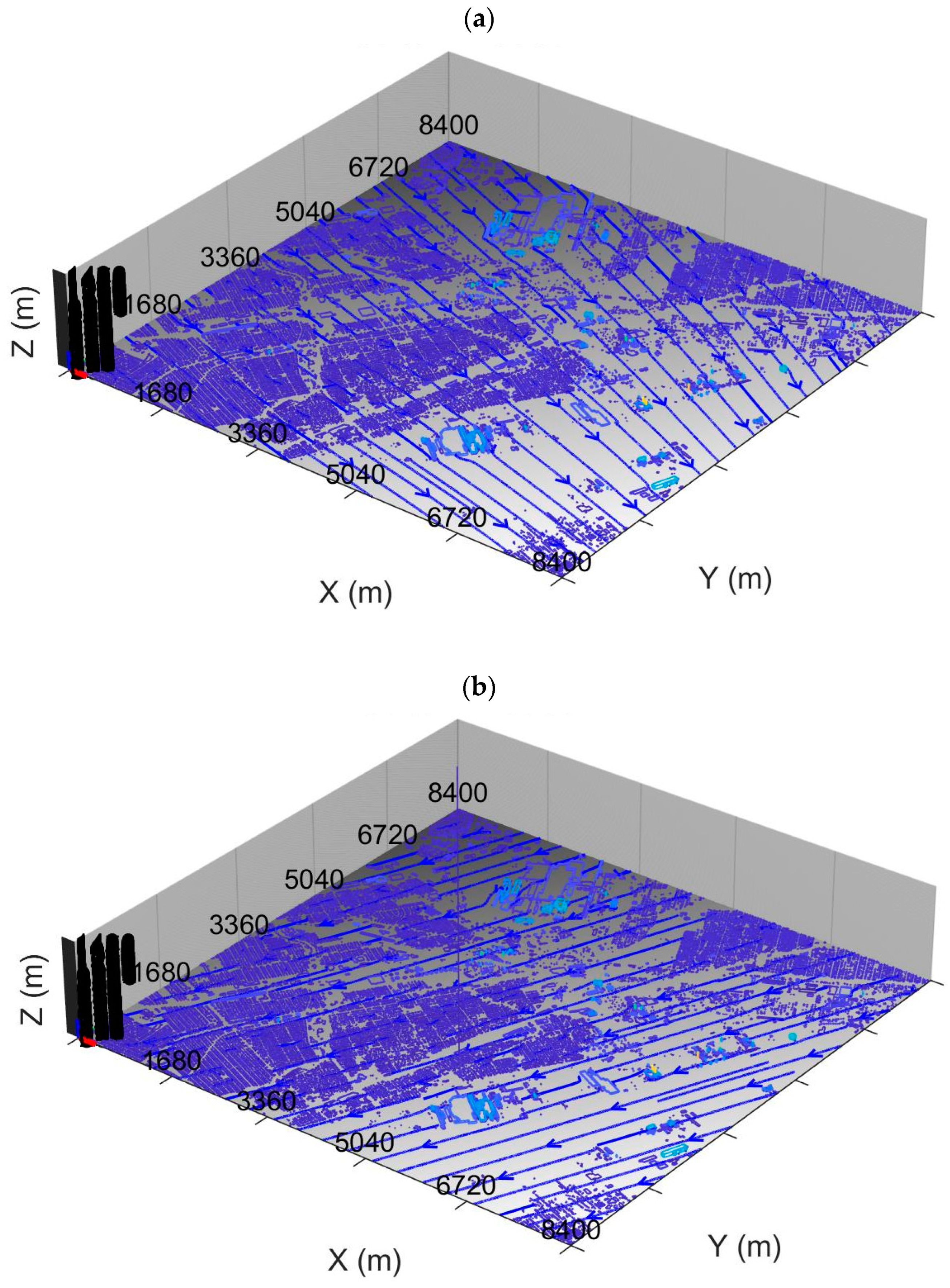
Figure 1 shows wind streamlines at a height of 1 m AGL generated by the QUIC model, constrained by wind data from the three EGLE monitoring stations in the Dearborn Loop plus the EGLE station at Allen Park near the southwest corner of the model domain. The prevailing wind speeds and directions are such that a pollutant signal can propagate across the entire MicroFACT domain within the simulation period so that an approximate concentration steady state is established at the end of each simulation (assuming steady emissions).
To calculate the planetary boundary layer (PBL) height, values of the surface temperature TS,j, and nominal surface wind speed US,j (where j is the simulation period) were specified from EGLE station measurements that best reflected the incoming air mass (Dearborn for j = 1 and Southwest Detroit for j = 2). Surface pressure, relative humidity, and cloud cover were specified based on reported conditions at the Detroit Metropolitan Wayne County (DTW) Airport. Values for the friction velocity, Monin–Obukhov length, and PBL height were derived from the turbulence parameterization described in the Supplementary Material of Olaguer et al. [23], assuming a surface roughness length of 0.1 m and the specified values of TS,j, US,j, and cloud cover. Table 1 summarizes the meteorological input parameters assumed in this study.
The layer temperatures above the surface were extrapolated from the surface temperature assuming the moist adiabatic lapse rate. The resulting vertical profile was used to compute temperature-dependent chemical reaction rates. Clear-sky photolysis rates were multiplied by the ratio of the measured solar radiation flux at the EGLE station in New Haven, Michigan (the nearest station where such measurements are available) to the corresponding clear-sky solar radiation flux obtained from www.meteoexploration.com (accessed on 8 March 2023).
The profile of vertical diffusivity was computed from the PBL height, the friction velocity, and the Monin–Obukhov length based on the urban diffusivity parameterization of Delle Monache et al. [24] as implemented by Olaguer et al. [12]. The horizontal diffusivity was set at a constant value of 50 m2/s as in Olaguer [16]. Dry deposition velocities for the 35 transported species were likewise set as in Olaguer [16] based on preceding literature.
The boundary conditions (BCs) for the air quality fields, which also serve as a uniform prior estimates of initial conditions, are from Olaguer [16] except as follows. For the three pollutants subject to inverse modeling, namely NO, HCHO, and CO, the BCs were derived from the minimum AML measurements during the simulation period. For the secondary pollutants, NO2 and O3, and for the volatile organic compounds (VOCs): isoprene, toluene, xylenes, acetaldehyde, and terpenes, the BCs were derived from averages of AML measurements during the simulation period. For the hydrocarbons: propene and 1,3-butadiene, BCs were derived from annual mean concentrations measured at the appropriate upwind EGLE station (Dearborn or Southwest Detroit). Lastly, BCs for HONO and HNO3 were taken from MOOSE measurements at the Trinity–St. Mark’s station on 12 June 2021, 9:31–14:39 LST regardless of the simulation period. Table 2 lists the relevant BCs and deposition velocities assumed for this study.
2.4. Initial Emissions Estimates
Initial estimates of point source emissions for CO, NOx (=NO + NO2), and VOCs were based on the 2017 US National Emissions Inventory (NEI) [25]. One exception was HCHO, for which initial estimates were based on process-specific emission ratios of HCHO to CO derived from available stack tests and field study measurements as described in Olaguer et al. [6]. Initial estimates for HONO were set at 0.8% of NOx emissions [16,26]. Point source emissions were assigned to vertical layers using calculated plume release heights based on reported stack data for each industrial facility emission point in the NEI within the model domain. The calculated plume release heights were averaged over each horizontal grid cell. Figure 2 shows the resulting distribution of plume release heights for Periods 1 and 2. Note that the red markers in the figure represent the locations of industrial facilities or EGLE monitoring sites (see Table 3).
The highest plume release heights in Figure 2 are associated with power generation, steel manufacturing, and coking facilities. These sites are either in the northwest section of the model domain or in the eastern section near the bank of the Detroit River.
The plume rise-adjusted emissions derived from the NEI were kept unchanged except for NO, HCHO, CO, and NO2. The emissions of the first three compounds were adjusted by inverse modeling based on AML measurements of their concentrations in ambient air. The emissions of NO2, while not directly subject to inverse modeling, were indexed to NO emissions such that the emissions ratio of NO to NOx for all elevated and ground-level sources was always 90%. Numerical experiments with wider sets of inversely modeled compounds beyond NO, HCHO, and CO did not significantly improve the solution quality.
To avoid biasing the inverse model results, the initial point source estimates from the NEI for NO, NO2, HCHO, and CO were first averaged over the entire horizontal domain. The domain-averaged values, denoted by for species i, were re-assigned to grid cells with non-zero plume release heights as the prior emissions estimates. Note that this method lowers the total domain emissions of each of the four compounds relative to the initial NEI-derived estimates. Overall, the prior emissions estimates are purposely conservative.
For stationary non-point sources of NOx and CO, total emissions in the model domain were set equal to the total NOx or CO point source emissions in the model domain multiplied by the ratio of Wayne County (NEI) non-point source emissions to Wayne County (NEI) point source emissions. These total emissions were then divided by the total number of horizontal grid cells. The result was assigned to each surface grid cell as a prior non-point source emissions estimate. The initial estimate for HCHO was obtained by conservatively multiplying the corresponding value for CO by a factor of 0.0002. Note that because marine vessels routinely operate in the Detroit River, no distinction was made between land and water grid cells in assigning non-point source emissions, which are presumed to be largely produced by combustion. Nevertheless, the possibility of significant non-combustion fugitive emissions of HCHO is considered in the inverse modeling adjustments of ground-level emissions.
Mobile source emissions were estimated by scaling county-level emissions computed using the Motor Vehicle Emission Simulator (MOVES) [27] according to the ratio of total road lengths in each model grid cell to the total road lengths in Wayne County. Biogenic emissions of isoprene were estimated from the high-resolution regional air quality model runs described in Olaguer et al. [6]. Grid cell-specific isoprene emissions of 0.024 US tons/year were assumed for Period 1, and 0.0072 US tons/year for Period 2.
2.5. Error Parameters
The 4Dvar method requires specification of certain error parameters. Some of these parameters were set independently of the simulation period. These include the assumed measurement errors for the three species subject to inverse modeling, and the corresponding prior estimates of the background concentration error covariances, which indicate the uncertainty in the initial conditions. These parameters are listed in Table 4.
In addition to the error parameters listed in Table 4, prior estimates of the emission error covariances must also be set to reflect uncertainties in the prior emissions estimates. These parameters are specific to each simulation period and were tuned to optimize the agreement between the forward model-predicted concentrations of the three inverse-modeled species and the corresponding grid cell-averaged ambient concentration measurements. Separate error covariances were assigned to elevated and ground-level emission sources.
The prior estimate of the point source emission error covariance for species i was applied only to elevated sources and is modeled in terms of the prior point source emissions estimate (see above), the cell-averaged plume release height (meters), and the tunable parameter as follows:
The prior estimate of the ground-level emission error covariance for species i was applied only to surface cells with no stacks present and is modeled in terms of the prior ground-level emissions estimate and the tunable parameter as follows:
In the case of NO and CO, Equation (2) was only applied when the maximum measured ambient concentration of NO in a grid cell exceeded 50 ppb or if the maximum measured ambient concentration of CO in the same grid cell exceeded 300 ppb. This was partially intended to represent transient vehicular traffic plumes beyond longer-term average mobile source emissions. For HCHO, the ground-level emission error covariance allows for non-combustion fugitive emissions that are not correlated with NO or CO emissions.
Note that the inverse modeling method used in this study combines automated emissions adjustments by the 4Dvar technique with the heuristic emissions tuning via the parameters and . The selected values of and are listed in Table 5. The lower values of these parameters for Period 2 relative to Period 1 may reflect a lower PBL height, less traffic emissions, or the disposition of sources relative to the prevailing winds.
2.6. Observed Ambient Concentrations
The AML sampling plan during MOOSE was largely, though not exclusively, focused on the chemical fingerprinting of point sources. Other objectives included co-location with EGLE monitoring stations during high ozone days, characterization of lake breeze front chemical conditions, and coordinated actions with other mobile laboratories. The Dearborn Loop was sampled during 12 of the 40 days that the AML was present in the SEMI region. The two simulation periods of interest to this study were selected because of the prevailing wind directions relative to the two EGLE monitoring stations with the most measurements (Dearborn and Southwest Detroit), and because they facilitated contrasting analyses of the emission sources within the Dearborn Loop area.
For this study, AML measurement records with over 150 ppb of NO or 1000 ppb of CO were filtered from the analysis. This was intended to remove interferences from individual motor vehicle plumes without eliminating the transient influences of mobile source fleets, as explained above.
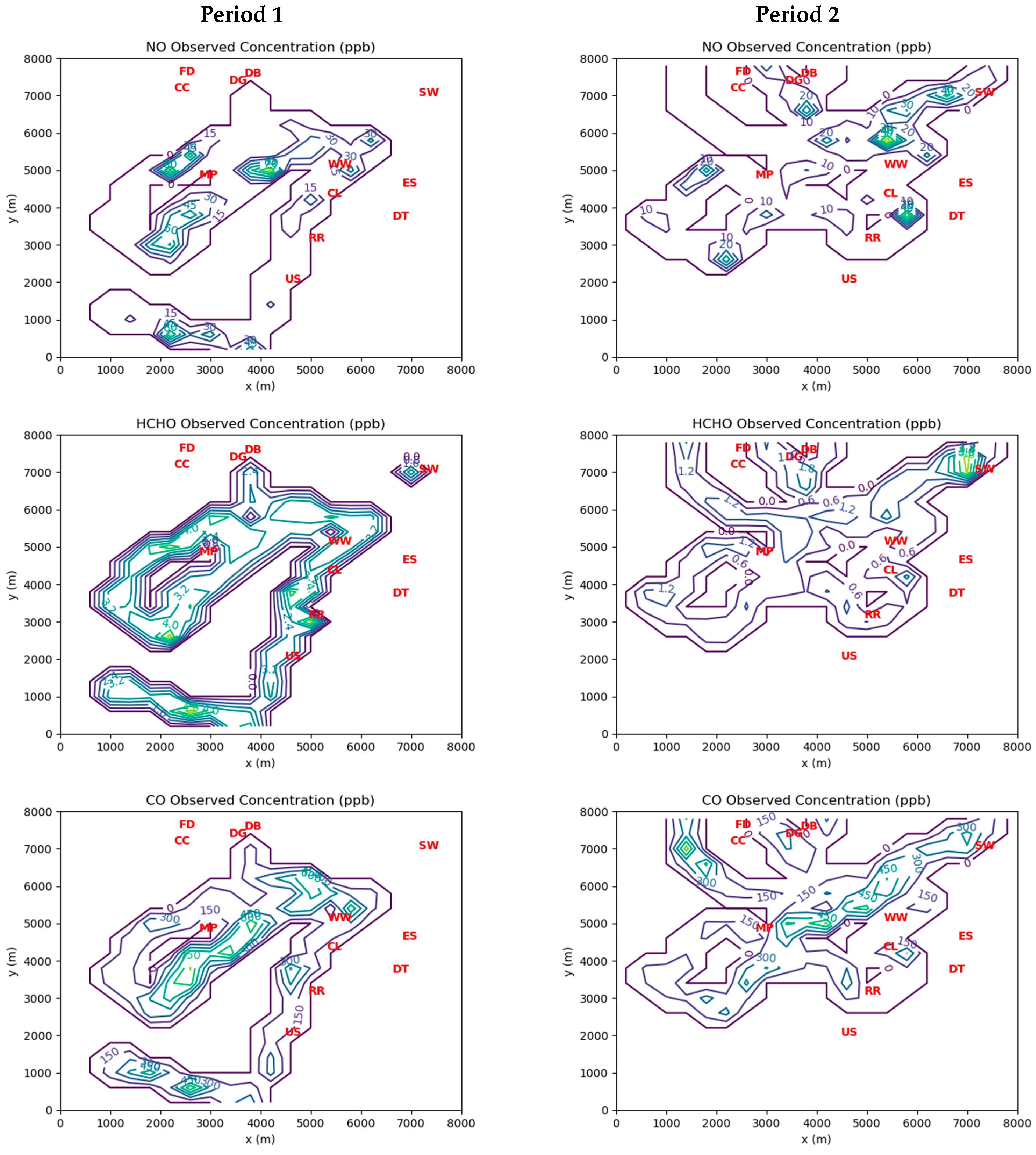
Figure 3 shows grid cell-averaged measurements of ambient concentrations of the three inverse-modeled species during Periods 1 and 2. Note that for Period 1 there were coincident 24 h average HCHO concentration measurements available at the Southwest Detroit and River Rouge monitoring stations. These measurements were treated as indicative of the hourly averages at those locations during Period 1. There were no corresponding station measurements available during Period 2, as carbonyls were only measured every 6 days at best.
There is a significant difference in the magnitudes of the measured ambient concentrations between the two periods of interest. Period 1 concentrations are much higher than those measured during Period 2. This is likely due to the significant influence of emissions from the industrial facilities at the northwest corner of the domain, which were upwind of the AML measurements during Period 1.
The cell-averaged ambient concentrations obtained from ~1 s frequency measurements by the AML were treated by the inverse model as constant during the data assimilation time window. The results of the MicroFACT modeling based on these observation-based inputs are discussed in the next section.
3. Results
3.1. Inferred Emissions
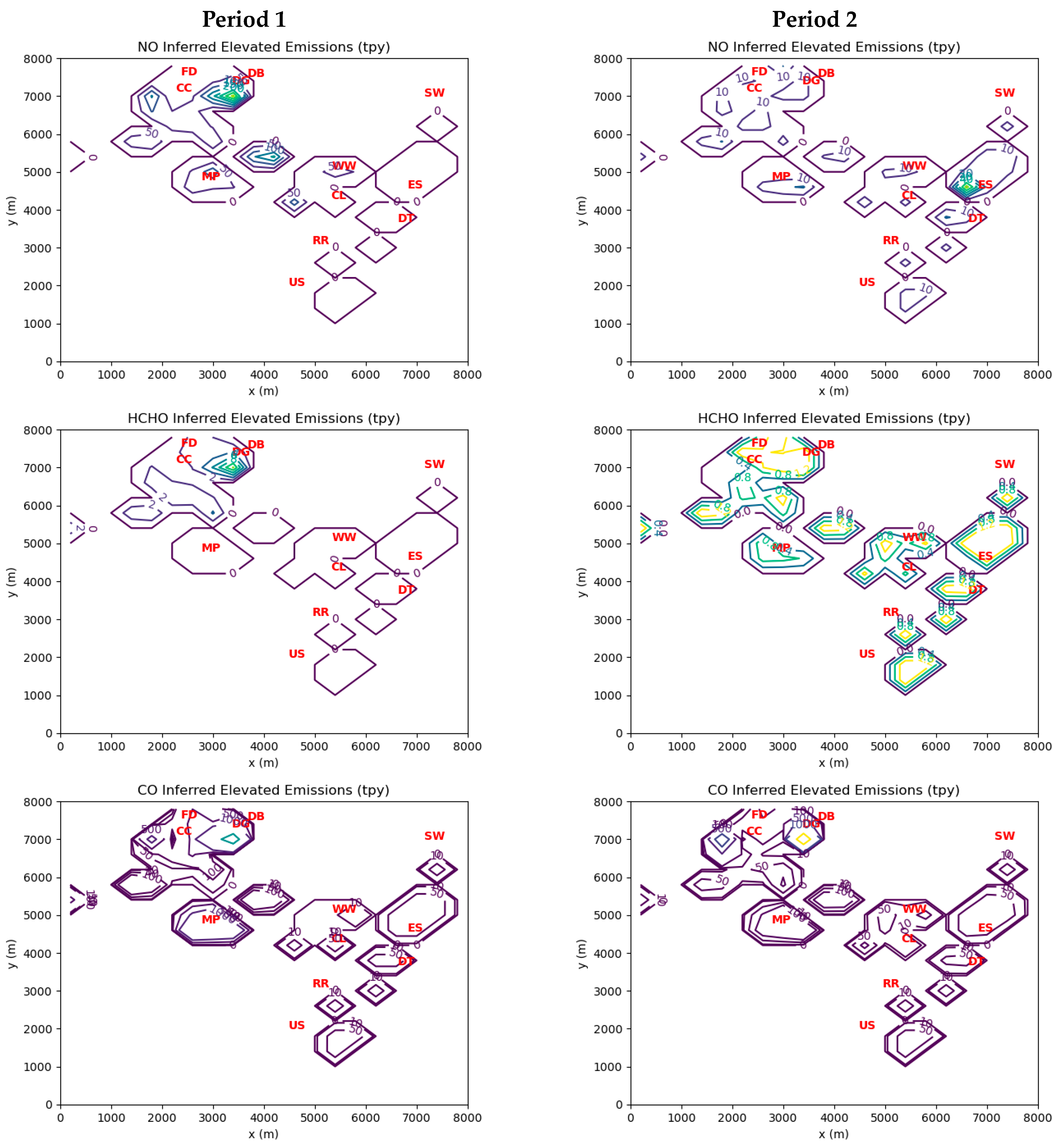
Figure 4 displays emissions inferred by MicroFACT for elevated sources. In Period 1, the influence of point sources in the vicinity of the Dearborn Industrial Generation clearly stands out. However, there is a weaker contribution from sources around Cleveland Cliffs and Marathon Petroleum. Maximum HCHO cell emissions for Period 1 are 12.2 US tons per year (tpy). During Period 2, elevated HCHO cell emissions of 1 tpy (maximum of 1.7 tpy) from the coking, power, steel, and waste treatment industries on the eastern side of the domain are comparable to the emissions on the northwest side.
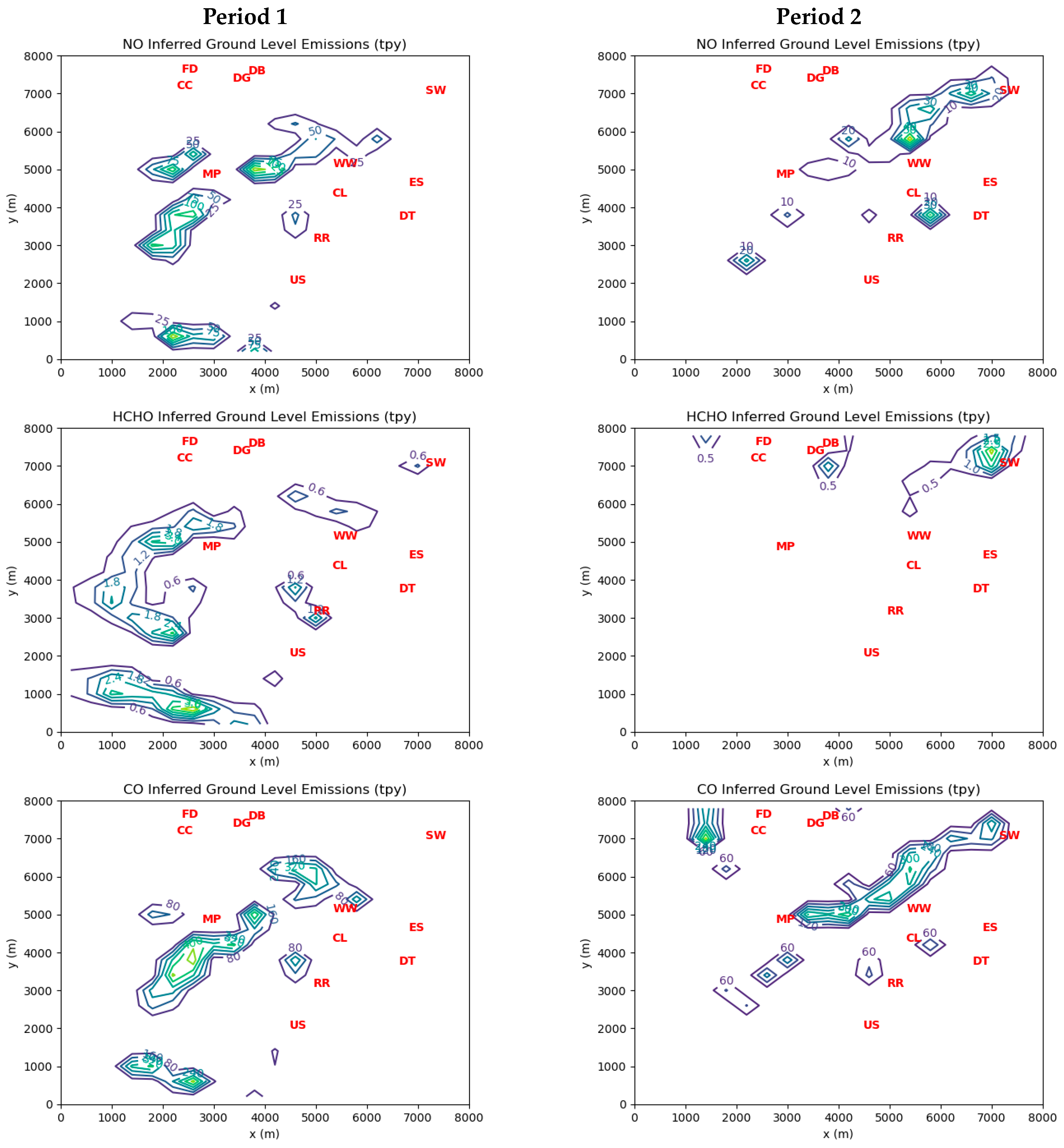
Figure 5 shows emissions inferred by the inverse model for ground-level sources. The contours of cell emissions during both periods have coherent large-scale structures that suggest the influence of mobile sources, such as industrial truck traffic. Maximum ground-level HCHO cell emissions are 4.8 tpy for Period 1 and 3.7 tpy for Period 2.
During Period 1, there were 40 grid cells with inferred elevated emissions greater than 1 tpy, for which the average HCHO:CO mass emission ratio was 5.2%. During the same period, there were 41 grid cells with inferred ground-level emissions greater than 1 tpy. Two cells had a HCHO:CO ratio greater than 1, suggesting that fugitive sources of HCHO were more important than combustion sources at these locations. The average ground-level HCHO:CO mass emission ratio for the remaining 39 grid cells during Period 1 was 2.2%. Similarly, during Period 2 the average HCHO:CO ratio for the 34 cells with elevated emissions greater than 1 tpy was 2.0%, while the seven cells with ground-level emissions greater than 1 tpy had an average ratio of 3.6%. The average HCHO:CO ratio for all grid cells was 2.4% for Period 1 and 0.4% for Period 2. These results confirm the assumption by Olaguer et al. [6] based on stack tests and other field data that incomplete combustion emissions from industrial sources apart from landfill-gas-fired stationary engines should typically yield HCHO:CO mass ratios between 2 and 10%.
3.2. Simulated Ambient Concentrations and Solution Quality
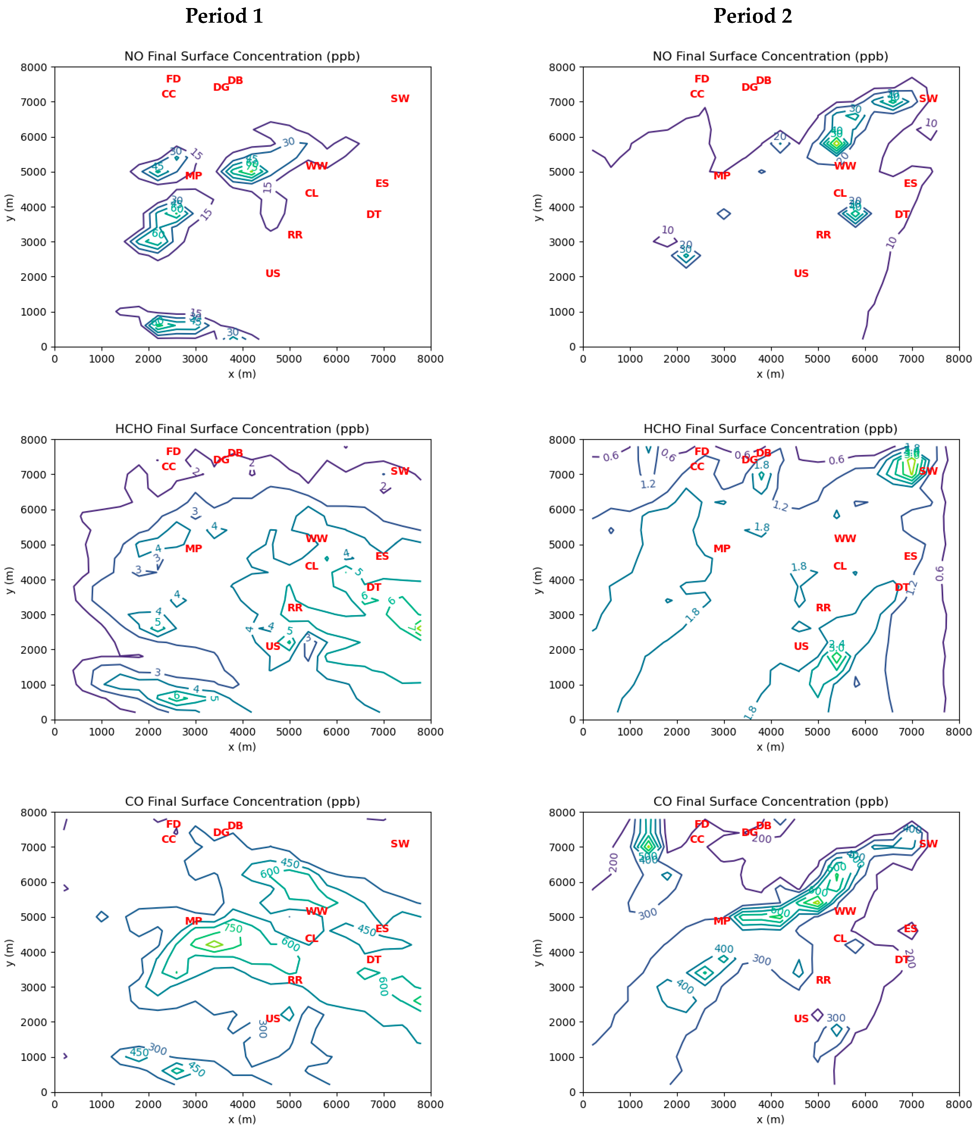
Figure 6 shows the final surface concentrations of NO, HCHO, and CO predicted by the MicroFACT model at the end of the two simulation periods based on the inferred emissions. During Period 1, there is a large portion of the model domain with ambient HCHO concentrations between 3 and 6 ppb, whereas during Period 2 ambient HCHO concentrations are mostly below 2 ppb, except on the eastern side near or downwind of the steel, coking, and power generation facilities, and in the vicinity of the Southwest Detroit monitoring station where the AML measured high ambient concentrations of HCHO during Period 2 (see Figure 3). Clearly, simulated HCHO exposures in the Dearborn Loop area depend significantly on wind direction relative to the largest sources.
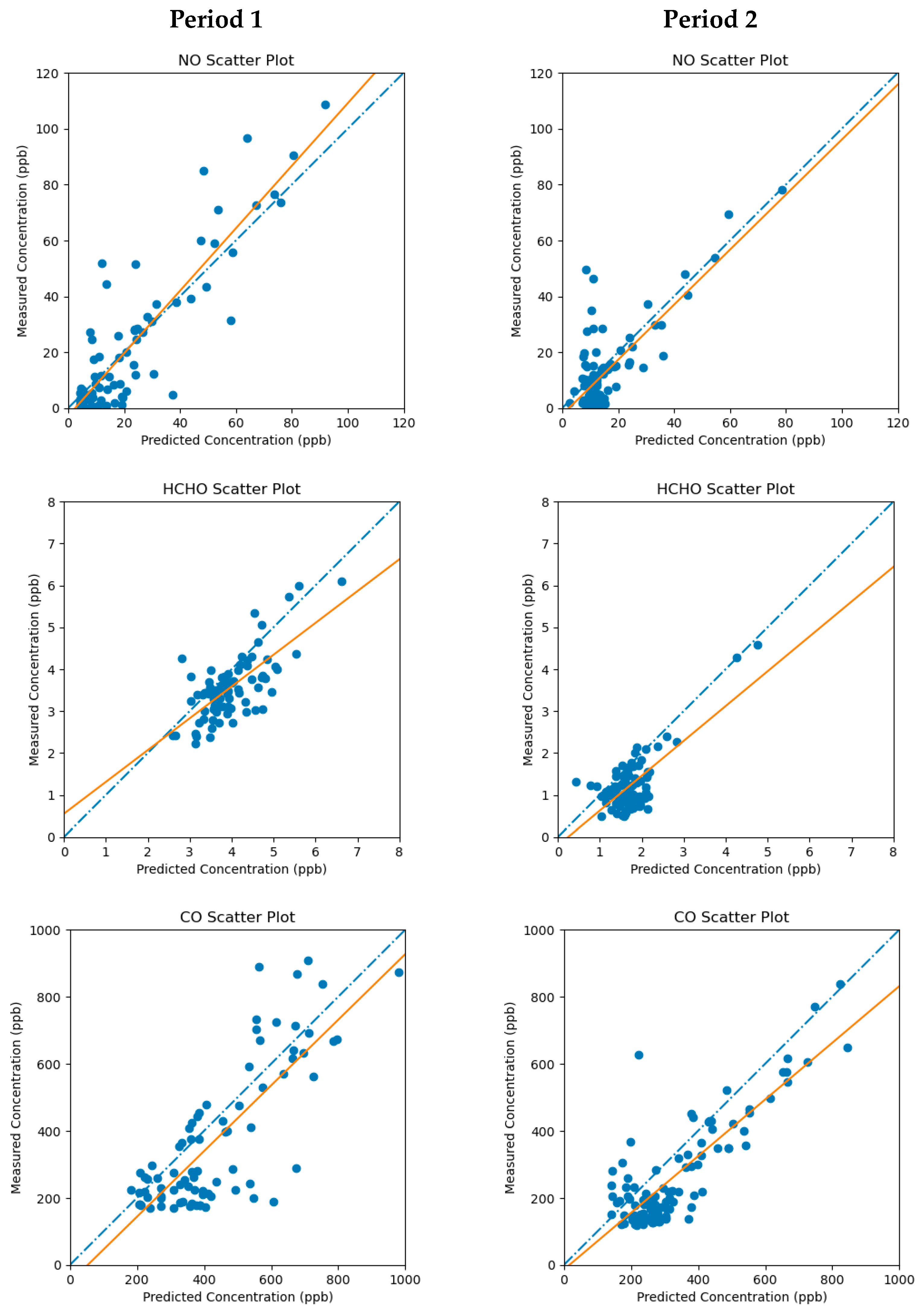
Figure 7 displays scatter plots and linear regressions of measured vs. predicted ambient concentrations for NO, HCHO, and CO during Periods 1 and 2, while Table 6 lists the regression parameters. The solution qualities are best for NO and CO, as their regression slopes and correlation coefficients are closest to 1. Because HCHO is as much a secondary pollutant as a directly emitted compound, it is more difficult to get a high-quality solution than for the primary pollutants, NO and CO. Nevertheless, the HCHO solution is acceptable, as the square of the Pearson correlation coefficient (r) is greater than 0.5, while the regression slope is still reasonably close to 1 for both simulation periods.
4. Discussion
The HCHO emissions estimated in this study stand in sharp contrast to the corresponding emissions obtained or inferred from reports to the State of Michigan in 2017 by industrial facilities in the Dearborn Loop area. Table 7 lists these facility emissions as recorded in the Michigan air emissions reporting system (MAERS), a public database maintained by EGLE [28]. The NOx, CO, and VOC emissions data in MAERS were the basis for the 2017 NEI data used to derive initial emissions estimates for the model. Note that the facilities in Table 7 are listed in order of their reported CO emissions. Except for Marathon Petroleum, these facilities have recorded HCHO emissions far below 1 tpy.
The underestimation of primary HCHO is caused by the corresponding emission factors in the USEPA’s AP-42 database [29] being out-of-date. However, in 2014 the USEPA made changes in VOC, NOx, and CO emission factors for flares and other units at refineries in response to legal action [30]. Moreover, emissions inventories usually do not include primary HCHO that is formed as a product of incomplete combustion (PIC) prior to release. As discussed by Olaguer et al. [6], these combustion emissions have been successfully measured in the field with contemporary ultraviolet/visible, and/or infrared spectroscopic techniques. Such field measurements, however, have mostly not been incorporated into emission factor determinations for HCHO.
As already mentioned, an important PIC co-emitted with HCHO is CO, although CO is itself an active agent in reducing NOx [31]. The maximum elevated cell emissions of CO inferred by this study were 7103 tpy (=14.2 million lbs/year) in Period 1 and 7608 tpy (=15.2 million lbs/year) in Period 2, while the maximum ground-level cell emissions were 542 tpy and 491 tpy for Periods 1 and 2, respectively. The magnitudes of the inferred point source emissions suggest that some of the reported CO emissions in Table 7 may be overestimates, especially for the two steel mills. Even if this were true, the application of typical HCHO:CO ratios would still yield HCHO emission estimates well over 1 tpy for these sources.
For NO, the maximum elevated cell emissions for Periods 1 and 2 were 366 tpy (=731,051 lbs/year) and 64 tpy (=128,580 lbs/year), respectively, while the corresponding maximum ground-level cell emissions were 169 tpy in Period 1 and 77 tpy in Period 2. As was the case for CO, the inferred point source emissions for NO are generally lower than the reported values in MAERS.
The levels of HCHO emissions inferred by the MicroFACT model may be sufficient to explain the ambient HCHO concentrations consistently measured at the three EGLE stations in the Dearborn Loop over the last two decades, as well as the concentration gradient between the Dearborn and River Rouge sites measured in 2021 (see Figure 6). While only two wind directions over two 1 h periods were simulated in this study, it is not difficult to see how different wind directions over a long period would alternate between the high exposure scenario of Period 1 and the low exposure scenario of Period 2. Figure 8 displays a wind rose based on measurements at DTW airport between 2018 and 2022. Northwesterly and northeasterly wind directions are prominent in the long-term data. In contrast, the dominant southwesterly wind direction should generate low HCHO exposures like those in Period 2, as the major emission sources would be downwind of or peripheral to most of the affected residential areas. Thus, the resulting long-term average HCHO exposures over the populated areas in the Dearborn Loop would likely be very similar to those indicated by the EGLE station measurements.
5. Summary and Conclusions
This study has demonstrated the feasibility and utility of inverse modeling for estimating widespread industrial emissions of chemically reactive compounds and quantifying cumulative exposure to HAPs with multiple primary and secondary sources. The results have practical implications for air quality policy and regulations because they identify a range of specific industrial sources that may be subject to controls to mitigate inhalation exposure to toxic HCHO and reduce the ambient concentrations and health impacts of criteria pollutants. These controls may include minimizing or improving the efficiency of flares, adding oxidation catalysts to stationary engines, and better detecting and capturing fugitive emissions.
The main conclusions drawn from this study are as follows:
- HCHO emissions from individual industrial facilities mainly representing the power, steel, coking, and waste treatment industries likely exceed 1 tpy.
- The average emission ratios of HCHO to CO in combustion sources emitting more than 1 tpy of HCHO are roughly 2 to 5%. This is consistent with known ratios from stack tests and other field measurements.
- Both elevated point sources and ground-level sources contribute significantly to ambient HCHO exposures.
- When winds favor the transport of emission plumes from the largest industrial sources towards the interior of the study area, widespread exposure to ambient concentrations of HCHO between 3 and 6 ppb may occur. Otherwise, ambient HCHO is mostly below 2 ppb (roughly the US national median) except in the vicinity or immediately downwind of large sources.
- Application of the MicroFACT model helped to explain the observed HCHO concentration gradient between the EGLE monitoring stations at Dearborn and River Rouge in 2021. The gradient arises because of the importance of primary HCHO on the local scale versus broader plumes of secondary HCHO, which would result in a more homogeneous distribution of ambient concentrations.
- Longer-term exposure to HCHO will result from a mix of favorable and unfavorable wind conditions, such that the measured long-term average HCHO concentrations at the three EGLE monitoring sites in the study area are likely good indicators of local population exposure.
In the future, the inverse model may be enhanced by utilizing automated techniques for estimating initial error covariances, such as pattern recognition (e.g., positive matrix factorization) or artificial intelligence, to distinguish source behaviors. This will minimize subjectivity and increase the accuracy of inverse modeling results. The cumulative impacts of HCHO including the enhancement of ambient ozone and PM2.5 would also be an important avenue for further investigation.
Supplementary Materials
The following supporting information can be downloaded at: https://www.mdpi.com/article/10.3390/atmos14060931/s1. Correction to Supplementary Material of Olaguer (2021). Equation (S1): substituting expressions for and .
Funding
This research was funded by the US Environmental Protection Agency, Washington, DC, USA, grant number XA00E02952.
Institutional Review Board Statement
Not applicable.
Informed Consent Statement
Not applicable.
Data Availability Statement
Related data for this study and other components of MOOSE can be found at https://www-air.larc.nasa.gov/missions/moose/index.html (accessed on 8 March 2023).
Acknowledgments
The author would like to thank Aerodyne Research, Inc. and its team led by Tara Yacovitch for providing the mobile laboratory data that was the basis for this study. The author also acknowledges EGLE staff members, Marissa Vaerten (M.V.), Tracey McDonald (T.M.), Rebekah Banura (R.B.), and Jim Haywood (J.H.), who provided emissions inventory data (M.V., T.M., R.B.) and Figure 8 (J.H.).
Conflicts of Interest
The author declares no conflict of interest.
References
- Zhou, Y.; Li, C.; Huijbregts, M.A.J.; Moiz Mumtaz, M. Carcinogenic air toxics exposure and their cancer-related health impacts in the United States. PLoS ONE 2015, 10, e0140013. [Google Scholar] [CrossRef] [PubMed]
- U.S. Environmental Protection Agency. Integrated Risk Information System (IRIS) on Formaldehyde; National Center for Environmental Assessment, Office of Research and Development: Washington, DC, USA, 1999.
- U.S. Environmental Protection Agency. Assessment Overview for the Toxicological Review of Formaldehyde—Inhalation [CASRN 50-00-0]; EPA/635/R-22/039c; Office of Research and Development: Washington, DC, USA, 2022.
- Calvert, J.G.; Orlando, J.J.; Stockwell, W.R.; Wallington, T.J. The Mechanisms of Reactions Influencing Atmospheric Ozone; Oxford University Press: New York, NY, USA, 2015. [Google Scholar]
- Dovrou, E.; Bates, K.H.; Moch, J.M.; Keutsch, F.N. Catalytic role of formaldehyde in particulate matter formation. Proc. Natl. Acad. Sci. USA 2022, 119, e2113265119. [Google Scholar] [CrossRef] [PubMed]
- Olaguer, E.P.; Hu, Y.; Kilmer, S.; Adelman, Z.E.; Vasilakos, P.; Odman, M.T.; Vaerten, M.; McDonald, T.; Gregory, D.; Lomerson, B.; et al. Is there a formaldehyde deficit in emissions inventories for southeast Michigan? Atmosphere 2023, 14, 461. [Google Scholar] [CrossRef]
- Michigan-Ontario Ozone Source Experiment (MOOSE). Available online: https://www-air.larc.nasa.gov/missions/moose/ (accessed on 8 March 2023).
- Marvin, M.R.; Wolfe, G.M.; Salawitch, R.J.; Canty, T.P.; Roberts, S.J.; Travis, K.R.; Aikin, K.C.; de Gouw, J.A.; Graus, M.; Hanisco, T.F.; et al. Impact of evolving isoprene mechanisms on simulated formaldehyde: An inter-comparison supported by in situ observations from SENEX. Atmos. Environ. 2017, 164, 325–336. [Google Scholar] [CrossRef]
- University of Michigan School of Public Health. The Southeast Michigan Chemical Source Signature (CHESS) Experiment, Final Report; Michigan Department of Environment, Great Lakes, and Energy: Lansing, MI, USA, 2023.
- Michigan Department of Environment, Great Lakes, and Energy. Michigan Air Quality Annual Report 2021; Michigan Department of Environment, Great Lakes, and Energy: Lansing, MI, USA, 2022.
- Olaguer, E.P. Application of an adjoint neighborhood scale chemistry transport model to the attribution of primary formaldehyde at Lynchburg Ferry during TexAQS II. J. Geophys. Res. Atmos. 2013, 118, 4936–4946. [Google Scholar] [CrossRef]
- Olaguer, E.P.; Herndon, S.C.; Buzcu-Guven, B.; Kolb, C.E.; Brown, M.J.; Cuclis, A.E. Attribution of primary formaldehyde and sulfur dioxide at Texas City during SHARP/formaldehyde and olefins from large industrial releases (FLAIR) using an adjoint chemistry transport model. J. Geophys. Res. Atmos. 2013, 118, 11317–11326. [Google Scholar] [CrossRef]
- Yacovitch, T.I.; Daube, C.; Lerner, B.; Claflin, M.; Fortner, E.; Canagaratna, M.; Herndon, S.C. Aerodyne Mobile Laboratory Measurements during the Chemical Source Signatures Experiment (CHESS): 2021 Michigan-Ontario Ozone Source Experiment (MOOSE), Final Report; Michigan Department of Environment, Great Lakes, and Energy: Lansing, MI, USA, 2022.
- Yacovitch, T.I.; Lerner, B.; Canagaratna, M.; Daube, C. Mobile Laboratory Investigations of Industrial Point Source Emissions during the MOOSE Field Campaign; Aerodyne Research, Inc.: Billerica, MA, USA, 2023. [Google Scholar]
- Chai, J.; Dibb, J.E.; Anderson, B.E.; Bekker, C.; Blum, D.E.; Heim, E.; Jordan, C.E.; Joyce, E.E.; Kaspari, J.H.; Munro, H.; et al. Isotopic evidence for dominant secondary production of HONO in near-ground wildfire plumes. Atmos. Chem. Phys. 2021, 21, 13077–13098. [Google Scholar] [CrossRef]
- Olaguer, E.P. The potential ozone impacts of landfills. Atmosphere 2021, 12, 877. [Google Scholar] [CrossRef]
- Colella, P.; Woodward, P.R. The piecewise parabolic method (PPM) for gas-dynamical simulations. J. Comput. Phys. 1984, 54, 174–201. [Google Scholar] [CrossRef]
- Smolarkiewicz, P.K. A fully multi-dimensional positive definite advection transport algorithm with small implicit diffusion. J. Comput. Phys. 1984, 54, 325–362. [Google Scholar] [CrossRef]
- Hertel, O.; Berkowicz, R.; Christensen, J. Test of two numerical schemes for use in atmospheric transport-chemistry models. Atmos. Environ. 1993, 27A, 2591–2611. [Google Scholar] [CrossRef]
- Zhang, S.; Sarwar, G.; Xing, J.; Chu, B.; Xue, C.; Arunachalam, S.; Ding, D.; Zheng, H.; Mu, Y.; Duan, F.; et al. Improving the representation of HONO chemistry in CMAQ and examining its impact on haze over China. Atmos. Chem. Phys. 2021, 21, 15809–15826. [Google Scholar] [CrossRef]
- Bocquet, M.; Elbern, H.; Eskes, H.; Hirtl, M.; Žabkar, R.; Carmichael, G.R.; Flemming, J.; Inness, A.; Pagowski, M.; Pérez Camaño, J.L.; et al. Data assimilation in atmospheric chemistry models: Current status and future prospects for coupled chemistry meteorology models. Atmos. Chem. Phys. 2015, 15, 5325–5358. [Google Scholar] [CrossRef]
- Singh, B.; Hansen, B.S.; Brown, M.J.; Pardyjak, E.R. Evaluation of the QUIC-URB fast response urban wind model for a cubical building array and wide building street canyon. Environ. Fluid Mech. 2008, 8, 281–312. [Google Scholar] [CrossRef]
- Olaguer, E.P.; Jeltema, S.; Gauthier, T.; Jermalowicz, D.; Ostaszewski, A.; Batterman, S.; Xia, T.; Raneses, J.; Kovalchick, M.; Miller, S.; et al. Landfill emissions of methane inferred from unmanned aerial vehicle and mobile ground measurements. Atmosphere 2022, 13, 983. [Google Scholar] [CrossRef]
- Delle Monache, L.; Weil, J.; Simpson, M.; Leach, M. A new urban boundary layer and dispersion parameterization for an emergency response modeling system: Tests with the Joint Urban 2003 data set. Atmos. Environ. 2009, 43, 5807–5821. [Google Scholar] [CrossRef]
- U.S. Environmental Protection Agency. National Emissions Inventory (NEI). Available online: https://www.epa.gov/air-emissions-inventories/national-emissions-inventory-nei#:~:text=The%20National%20Emissions%20Inventory%20(NEI,pollutants%20from%20air%20emissions%20sources (accessed on 8 March 2023).
- Kleffmann, J.; Kurtenbach, R.; Lörzer, J.C.; Wiesen, P.; Kalthoff, N.; Vogel, N.; Vogel, B. Measured and simulated vertical profiles of nitrous acid. Part I: Field measurements. Atmos. Environ. 2003, 37, 2949–2955. [Google Scholar] [CrossRef]
- U.S. Environmental Protection Agency. MOVES3 Technical Guidance: Using MOVES to Prepare Emission Inventories for State Implementation Plans and Transportation Conformity; EPA-420-B-20-052; Office of Transportation and Air Quality: Washington, DC, USA, 2020.
- Michigan Department of Environment, Great Lakes, and Energy. MAERS—Michigan Air Emissions Reporting System. Available online: https://www.egle.state.mi.us/maersfacility/Pages/Main/Login.aspx?ReturnUrl=%2fmaersfacility%2fdefault.aspx (accessed on 8 March 2023).
- U.S. Environmental Protection Agency. AP-42: Compilation of Air Emissions Factors. Available online: https://www.epa.gov/air-emissions-factors-and-quantification/ap-42-compilation-air-emissions-factors (accessed on 8 March 2023).
- U.S. Environmental Protection Agency. New and Revised Emissions Factors for Flares and New Emissions Factors for Certain Refinery Process Units and Determination for No Changes to VOC Emissions Factors for Tanks and Wastewater Treatment Systems. Available online: https://www.epa.gov/air-emissions-factors-and-quantification/new-and-revised-emissions-factors-flares-and-new-emissions (accessed on 8 March 2023).
- Song, J.; Wang, Z.; Cheng, X.; Wang, X. State-of-art review of NO reduction technologies by CO, CH4 and H2. Processes 2021, 9, 563. [Google Scholar] [CrossRef]
Figure 1.
Wind streamlines (dark blue arrows) at 1 m AGL generated by the QUIC model for the Dearborn Loop area during (a) 22 May 2021, 13:13–14:13 LST and (b) 30 May 2021, 10:00–11:00 LST. Light blue colors indicate taller structures.
Figure 1.
Wind streamlines (dark blue arrows) at 1 m AGL generated by the QUIC model for the Dearborn Loop area during (a) 22 May 2021, 13:13–14:13 LST and (b) 30 May 2021, 10:00–11:00 LST. Light blue colors indicate taller structures.

Figure 2.
Cell-averaged plume release heights inferred from point source stack data for Period 1 (left) and Period 2 (right). See Table 4 for interpretation of red markers.
Figure 2.
Cell-averaged plume release heights inferred from point source stack data for Period 1 (left) and Period 2 (right). See Table 4 for interpretation of red markers.

Figure 3.
Contours of cell-averaged AML measurements for ambient concentrations of NO, HCHO, and CO during Period 1 and Period 2. See Table 4 for interpretation of red markers.
Figure 3.
Contours of cell-averaged AML measurements for ambient concentrations of NO, HCHO, and CO during Period 1 and Period 2. See Table 4 for interpretation of red markers.

Figure 4.
Inverse model-inferred emissions of NO, HCHO, and CO in US tons per year (tpy) for elevated sources during Periods 1 and 2. Note that contours for CO are for 10, 50, 100, 500, 1000, and 5000 tpy. See Table 4 for interpretation of red markers.
Figure 4.
Inverse model-inferred emissions of NO, HCHO, and CO in US tons per year (tpy) for elevated sources during Periods 1 and 2. Note that contours for CO are for 10, 50, 100, 500, 1000, and 5000 tpy. See Table 4 for interpretation of red markers.

Figure 5.
Contours of inverse model-inferred emissions of NO, HCHO, and CO in US tons per year (tpy) for ground-level sources during Period 1 and Period 2. See Table 4 for interpretation of red markers.
Figure 5.
Contours of inverse model-inferred emissions of NO, HCHO, and CO in US tons per year (tpy) for ground-level sources during Period 1 and Period 2. See Table 4 for interpretation of red markers.

Figure 6.
Contours of model-predicted ambient concentrations for NO, HCHO, and CO at the end of Periods 1 and 2. See Table 4 for interpretation of red markers.
Figure 6.
Contours of model-predicted ambient concentrations for NO, HCHO, and CO at the end of Periods 1 and 2. See Table 4 for interpretation of red markers.

Figure 7.
Scatter plots and linear regressions (orange lines) of measured vs. predicted ambient concentrations for NO, HCHO, and CO during Period 1 and Period 2. The 1:1 lines are represented by the blue dot-dashes.
Figure 7.
Scatter plots and linear regressions (orange lines) of measured vs. predicted ambient concentrations for NO, HCHO, and CO during Period 1 and Period 2. The 1:1 lines are represented by the blue dot-dashes.

Figure 8.
Wind rose based on 5 years of meteorological data (2018 to 2022) from DTW airport.


Table 1.
Meteorological input parameters.
| Parameter | Simulation Period 1 | Simulation Period 2 |
|---|---|---|
| Surface Temperature | 298.10 K | 288.15 K |
| Surface Pressure | 1.002 atm | 1.002 atm |
| Relative Humidity | 47% | 37% |
| Cloud Cover | 30% | 50% |
| Nominal Surface Wind Speed | 8 m/s | 3 m/s |
| Friction Velocity | 0.72 m/s | 0.315 m/s |
| Monin–Obukhov Length | −194 m | −18.9 m |
| PBL Height | 1407.6 m | 407.5 m |
| Surface Roughness Length | 0.1 m | 0.1 m |
| Solar Radiation | 820.65 W/m2 | 875.46 W/m2 |
| Clear Sky Solar Radiation | 947.8 W/m2 | 900 W/m2 |
Table 2.
Chemical boundary conditions and deposition velocities for transported species.
| Chemical Species | Symbol | Boundary Condition (ppb) | Deposition Velocity (cm/s) | |
|---|---|---|---|---|
| Period 1 | Period 2 | |||
| Nitric Oxide | NO | 0.001 | 0.002 | |
| Nitrogen Dioxide | NO2 | 6.88 | 5.20 | 0.36 |
| Ozone | O3 | 55.7 | 43.1 | 0.42 |
| Nitrous Acid | HONO | 1.64 | 1.64 | 1.9 |
| Formaldehyde | HCHO | 1.20 | 0.008 | 0.54 |
| Carbon Monoxide | CO | 150.4 | 115.6 | |
| Ethene | C2H4 | 0.734 | 0.734 | |
| Propene | C3H6 | 0.71 | 0.77 | |
| 1,3-Butadiene | C4H6 | 0.02 | 0.03 | |
| 1-Butene | BUT1ENE | 0.02 | 0.02 | |
| 2-Butenes | BUT2ENE | 0.075 | 0.075 | |
| Isobutene | IBUTENE | 0.02 | 0.02 | |
| Isoprene | ISOP | 0.508 | 0.179 | |
| Toluene | TOL | 0.74 | 0.339 | |
| Xylenes | XYL | 0.35 | 0.147 | |
| Organic Nitrates | RNO3 | 0.701 | 0.701 | 0.32 |
| Paraffinic Bond | PAR | 27.9 | 27.9 | |
| Acetaldehyde | CH3CHO | 0.074 | 0.022 | 0.2 |
| Methacrolein + MVK 1 | ISPD | 0.508 | 0.508 | 0.2 |
| Peroxyacetyl Nitrate | PAN | 0.785 | 0.785 | 0.27 |
| Methane | CH4 | 1904 | 1904 | |
| Methanol | MEOH | 2.20 | 2.20 | 0.7 |
| Ethanol | ETOH | 0.697 | 0.697 | 0.6 |
| Nitric Acid | HNO3 | 0.66 | 0.66 | 2.7 |
| Terpenes | TERP | 0.635 | 0.022 | |
| Ethane | C2H6 | 1.58 | 1.58 | |
| Ketone Bond | KET | 5.42 | 5.42 | |
| Glyoxal | GLY | 0.165 | 0.165 | |
| Methyl Glyoxal | MGLY | 0.147 | 0.147 | 0.2 |
| Unsaturated Aldehyde 2 | OPEN | 0.0234 | 0.0234 | |
| Unsaturated Ketone 2 | XOPN | 0.0165 | 0.0165 | |
| Cresol | CRESOL | 0.0191 | 0.0191 | 0.2 |
| Higher Aldehyde | ALDX | 0.596 | 0.596 | |
| Higher Peroxyacyl Nitrate | PANX | 0.290 | 0.290 | 0.4 |
| NO3 + N2O5 | NO3X | 0.000696 | 0.000696 | 2.7 |
1 MVK = methyl vinyl ketone. 2 Product of aromatic ring decomposition.
Table 3.
Abbreviations for EGLE monitoring stations and notable industrial facilities.
| EGLE Monitoring Stations | |
| Dearborn | DB |
| Southwest Detroit | SW |
| River Rouge | RR |
| Industrial Facilities | |
| Ford Dearborn (automotive assembly) | FD |
| Dearborn Industrial Generation (power) | DG |
| Cleveland Cliffs (steel mill) | CC |
| Marathon Petroleum (refinery) | MP |
| Great Lakes Water Authority (wastewater treatment) | WW |
| Carmeuse Lime (lime producer) | CL |
| EES Coke (coking facility) | ES |
| DTE Energy (power) | DT |
| US Steel (steel mill) | US |
Table 4.
Inverse model error parameters.
| Chemical Species | Measurement Error (ppb) | Background Concentration Error Covariance (μg/m3)2 |
|---|---|---|
| NO | 1.0 | 2500 |
| HCHO | 0.3 | 16 |
| CO | 50.0 | 2500 |
Table 5.
Emission error covariance parameters.
| Chemical Species | ||||
|---|---|---|---|---|
| Period 1 | Period 2 | Period 1 | Period 2 | |
| NO | 0.001 | 0.0002 | 0.00015 | 0.00005 |
| HCHO | 0.005 | 0.0004 | 22.0 | 9.0 |
| CO | 0.1 | 0.005 | 0.02 | 0.01 |
Table 6.
Slope, intercept, and Pearson correlation coefficient (r) from linear regression analysis.
| Chemical Species | Period 1 | Period 2 | ||||
|---|---|---|---|---|---|---|
| Slope | Intercept | r | Slope | Intercept | r | |
| NO | 1.12 | −2.81 | 0.887 | 0.99 | −2.40 | 0.772 |
| HCHO | 0.76 | 0.55 | 0.708 | 0.83 | −0.20 | 0.728 |
| CO | 0.98 | −52.0 | 0.789 | 0.85 | −13.5 | 0.836 |
Table 7.
2017 data from the Michigan air emissions reporting system (MAERS).
| Facility | NOx (lbs/year) | CO (lbs/year) | VOC (lbs/year) | HCHO (lbs/year) |
|---|---|---|---|---|
| AK Steel (Cleveland Cliffs) Dearborn Works | 756,406 | 33,105,096 | 96,759 | 12 |
| US Steel Great Lakes Works | 1,960,104 | 29,811,671 | 103,421 | 117 |
| EES Coke Battery LLC | 2,701,308 | 809,502 | 179,943 | 0 |
| Dearborn Industrial Generation | 1,052,385 | 563,358 | 29,500 | 324 |
| Carmeuse Lime, Inc. River Rouge Operation | 869,008 | 420,488 | 0 | 0 |
| DTE Electric Company River Rouge Power Plant | 3,038,094 | 351,680 | 10,059 | 13 |
| Marathon Petroleum Company LP | 776,493 | 316,764 | 685,307 | 9349 |
| Great Lakes Water Authority | 297,272 | 155,894 | 26,015 | 2 |
| Ford Motor Company Rouge Complex | 128,684 | 28,825 | 1,635,947 | 4 |
Disclaimer/Publisher’s Note: The statements, opinions and data contained in all publications are solely those of the individual author(s) and contributor(s) and not of MDPI and/or the editor(s). MDPI and/or the editor(s) disclaim responsibility for any injury to people or property resulting from any ideas, methods, instructions or products referred to in the content. |
© 2023 by the author. Licensee MDPI, Basel, Switzerland. This article is an open access article distributed under the terms and conditions of the Creative Commons Attribution (CC BY) license (https://creativecommons.org/licenses/by/4.0/).
Share and Cite
MDPI and ACS Style
Olaguer, E.P. Inverse Modeling of Formaldehyde Emissions and Assessment of Associated Cumulative Ambient Air Exposures at Fine Scale. Atmosphere 2023, 14, 931. https://doi.org/10.3390/atmos14060931
AMA Style
Olaguer EP. Inverse Modeling of Formaldehyde Emissions and Assessment of Associated Cumulative Ambient Air Exposures at Fine Scale. Atmosphere. 2023; 14(6):931. https://doi.org/10.3390/atmos14060931
Chicago/Turabian StyleOlaguer, Eduardo P. 2023. "Inverse Modeling of Formaldehyde Emissions and Assessment of Associated Cumulative Ambient Air Exposures at Fine Scale" Atmosphere 14, no. 6: 931. https://doi.org/10.3390/atmos14060931
Note that from the first issue of 2016, this journal uses article numbers instead of page numbers. See further details here.