3.1. Puzzling Observations in the MATERHORN Campaign
The detailed results concerning nocturnal turbulence observed during the MATERHORN campaign were published in a series of papers [
5,
11,
12]. In these studies, different data analyses and presentation methods were employed, viz., the spectral approach in Fourier space [
12] and the structure functions approach in physical space [
4]. Although both approaches are inter-related, each of them better reflects specific features of nocturnal turbulence. In particular, a small-scale bursting phenomenon was uncovered using the spectral approach [
12], and the celebrated Kolmogorov −5/3 spectrum appropriately described the measured spectral behavior in the inertial subrange for so-called no-bursting intervals, where “bursts” were effectively removed from the time series using proper thresholds based on KE dissipation. At the same time, the structure functions approach enabled the discovery of inertial and viscous (dissipation) subintervals with separate, corresponding power exponents for the bursting and no-bursting intervals. In this paper, we limit ourselves to the time series where the bursting events are removed.
In particular, our recent paper [
4], on the stably stratified turbulence occurring in the nocturnal turbulence observed during MATERHORN [
11,
12], reported an unexpected behavior of the canonical (normalized) third-order longitudinal structure function (
Figure 1).
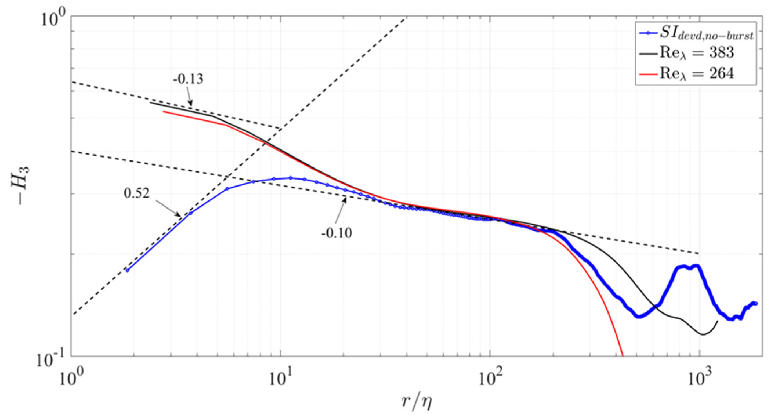
In
Figure 1, the canonical third-order structure function measured at a 6 m height from the ground was compared with the same structure functions evaluated for nearly isotropic turbulence obtained by classical box DNS computations [
14]. In the field, the
Reλ was 1250, whereas in the DNS computations the
Reλ was 264 and 383. While in the inertial subrange (
r/η = 20 ÷ 200), both the qualitative and quantitative agreements were very good, in the viscous subrange (
r/η ≤ 10) the results were conspicuously different, and the difference increased with the decrease in separation. It is worth noting that at small normalized separations
r/η < 10, the scaling exponents were even of different signs for the field and DNS data. Since, in the viscous subrange, one can expect linear dependence between velocity and separation, e.g., [
15], the scaling exponent for the conventional third-order structure function should be about zero to satisfy Kolmogorov’s Self-Similar Hypothesis (KSSH) [
16].
This difference of scaling exponents in the viscous subrange of field experiments and DNS is puzzling, especially when there is a clear agreement among the scaling exponents in the inertial subrange with each other and with the Kolmogorov inertial subrange scaling. To shed light on this perplexing behavior, the canonical normalized third-order structure function was computed at various separations; it is defined as the third-order structure function
L3 divided by the second-order structure function
L2 to the power 1.5, e.g.,
, which also represents the skewness of the structure function. In
Figure 2, we separately consider the third- and second-order structure functions, both normalized according to KSSH [
16].
The third-order structure function in
Figure 2a yields, in the viscous subrange, the expected linear dependence of the characteristic velocity increment
on the separation
r, e.g.,
~
r1. However, the second-order structure function in
Figure 2b corresponds to a different type of dependence, namely,
~
r5/6. This explains the scaling exponent observed for the canonical third-order structure function in
Figure 1.
However, as shown in
Figure 1, the power exponent of the canonical structure function is relatively small, ~−0.1 in the DNS computations of the approximately homogeneous isotropic turbulence, compared to ~+0.5 obtained in the field experiment. The determination of the separate scaling exponents from the DNS data, in a manner similar to that of the field data, as shown in
Figure 2, yielded the following dependencies,
~
r0.87 for third-order and
~
r0.91, for second-order structure functions. It is worth noting that the expectation of identical behavior by odd and even structure functions is generally unjustified, despite it being widely quoted and often used, in particular, in the Extended Self-Similarity (ESS) approach. In previous research [
4], we found that all even (second, fourth, and sixth in this study) structure functions yield
~
r5/6 in the viscous subrange. Then, it was found that all the odd structure functions (first, third, and fifth in this study) constructed using the modulus of velocity increment
yield a similar relation, namely,
~
r5/6 in the viscous subrange; here,
is the characteristic velocity increment at selected separation
r. The consistent and significant difference between the power exponents of the third- and second-order structure functions is responsible for the substantial power exponent 0.5 at the small scales of the conventional third-order structure function/skewness. In isotropic DNS, this power exponent is about −0.1, which is much closer to zero, though of a different sign. This result is somewhat perplexing, given the expectation that, due to the local isotropy at small scales, the power exponent tends to be zero. Even more puzzling is that, in the inertial subrange, the behavior of the canonical third-order structure function in the DNS and field experiments shows full (qualitative and quantitative) agreement.
This apparently contradicts with the postulate of local isotropy (PLI), which entails better isotropy whence the separation (
r/η) is diminishing. Cambon et al. [
17], however, predicted such behavior in cases where external anisotropic forces such as rotation (Coriolis) and stable stratification (buoyancy) do not produce turbulent energy. In particular, they state the following: “It is often considered that anisotropy only affects the largest scales of the turbulent flow, so that the cascade of anisotropy only mildly penetrates toward the scales in the inertial range, with eventually no direct impact on the dissipative range, according to the view inherited from Kolmogorov [
16]. In this scheme, the large-scale anisotropy induced by body forces and/or mean gradients is just considered as a particular modality of ‘forcing’ the largest scales. This viewpoint is radically questioned for flows in which the body force responsible for anisotropy is energy conserving.” Moreover, they state that “Anisotropy develops from isotropic initial conditions due to nonlinear energy transfer towards the plane of zero frequency in wave-vector space. However, two-dimensionalization does not occur: the fraction of energy at or near the zero-frequency plane remains small at all times. The cascade to small scales is strongly anisotropic, producing angle-dependent spectra which become more and more (not less) anisotropic, the smaller the scale considered”.
Obviously, in shear flows, turbulent energy is produced, notwithstanding, the laboratory experiments with homogeneous shear flow by Warhaft and their co-workers [
18,
19,
20] unambiguously showed that the return to isotropy expected at the small scales does not occur either at a lower
Reλ~O(100) [
18] or at a higher
Reλ~O(1000) [
19], which was again ascribed to shear penetrating to smaller scales. To quote [
19], “The results show that PLI is untenable, both at the dissipation and inertial scales, at least to
Rλ~1000, and suggest it is unlikely to be so even at higher Reynolds numbers.” See more considerations in the Discussion section.
Our results [
4] appear to strongly support the observation that stratified turbulence differs from nearly isotropic turbulence, even at small scales corresponding to the dissipation (viscous) sublayer, and raise a question about the PLI for this important case. It was very desirable to assert the validity of our results by independent measurements at a higher
Reλ~O(1000) or the DNS computations of stably stratified turbulence.
Unfortunately, the laboratory experiments of stably stratified turbulence are limited to a relatively low
Reλ (<100), and, thus, high-quality field experiments with continuous measurements at high sampling rates are called for. In fact, during the entire MATERHORN campaign, only a few records provided “clean” data sets for the nocturnal stably stratified turbulence strongly affected by thermal stratification. It should be stressed that these measurements were possible due to our novel calibration approach that enabled in situ calibration of a multi-hot-film probe based on the simultaneous measurements of low-frequency 3D-velocity data of a collocated sonic anemometer. Employing machine learning (neural network training) enabled the calibration of the hot-film probe in situ, thus avoiding problems with the hot-film’s potential deterioration in hostile field environments. The efficacy of this calibration method [
21] was tested in a series of papers [
22,
23,
24] and proved to be very efficient, even in the presence of noise to some degree.
In the current work, the neural network procedure was based on the Multi-Layer Perceptron (MLP) approach. MLP contains one input layer, one or two hidden layers, and one output layer. The number of nodes of the input layer and the number of input signals are the same. We used a fully connected network. In this case, each node of the input layer duplicates and sends its input signal to every neuron of the first hidden layer. The hidden layer consists of a number h of neurons. For the training of MLP, the Back Propagation and Conjugate Gradient Descent methods were sequentially used. In all cases, the number of epochs that was necessary for the generation of the neural network did not exceed 100.
The use of two collocated x-probes (oriented in the horizontal and vertical planes) at a very small separation allowed for the measurement of the full 3D velocity vector. Via the Taylor hypothesis, the time series of the velocity components could be converted into a velocity series in the mean wind direction. As expected, the processed data records were limited in time (about 1 min) to keep the mean transverse velocity components as small as possible. Directly after the end of the record, the probe was aligned with the mean horizontal velocity that was evaluated during the last 5 s of the record. Each record was flagged as successful if the mean wind direction differed by less than 10° from its value at the beginning of the record.
Stratified turbulence is essentially anisotropic (at least at large scales) and is characterized by horizontal pancake-like layering; thus, we posit that the surprising result observed in
Figure 1 is related to anisotropy and layering. The DNS of the stably stratified turbulent flow in a box could help in this regard, notwithstanding its idealized nature. DNS simulations were conducted by Jack Herring in collaboration with Yoshi Kimura and were presented in two seminal papers, one in the
Journal of Fluid Mechanics [
2] and the other in
Physica Scripta [
25]. The significance of their work is limited not only to the very detailed and comprehensive presentations of the spectra and structure functions obtained at a relatively high
Reλ but also to the elegant methodology of velocity data analysis based on Craya–Herring decomposition. The latter approach allows for the separation of the entire oscillating flow into 2 types of modes: horizontal and
vortical; vertical and
wavy [
2,
23]. In
Section 3.2, the puzzling results (the penetration of the anisotropy caused by stratification into small scales) of our study are discussed in light of [
2].
3.2. DNS of Stably Stratified Turbulence by Kimura and Herring 2012 [2]
As shown in [
2], the second-order structure function
St2(d, u, x) for the longitudinal velocity component
u at separation
d (
r in our notations) in the
x-direction can be presented as the superposition of two terms following Craya–Herring decomposition (expression 4.4 in [
2]).
where
and
are defined as energy densities; the
k⊥ and
kz components of vector number
k are in the horizontal plane and the vertical direction, respectively; and
J0 and
J1 denote the Bessel function of the corresponding order. While
contributes only to velocities in the horizontal plane and is determined by vertical vorticity component
ωz,
is contributing to both horizontal and vertical velocity components and can be determined using only the vertical velocity component
w, as presented in expressions 2.9 and 2.10, respectively [
2]. Since, in a stratified flow, the vertical direction coincides with gravitational acceleration
g, the second term of the decomposition may account for the internal waves. Indeed, the behavior of the second-order structure function due to the first term only, evaluated in [
2], is practically the same as that of the isotropic turbulence (see Figure 14 in [
2]), while adding the second term accounting for buoyancy leads to behavior of the second-order structure function that substantially differs from that of the isotropic turbulence.
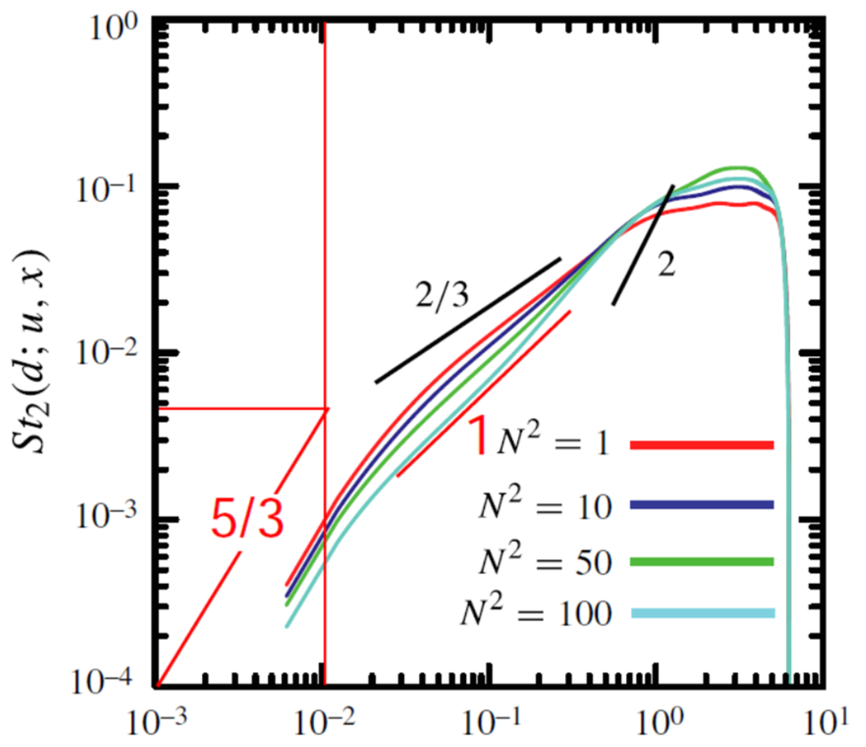
The second-order longitudinal structure function in the
x-direction (see Figure 15a in [
2]) is shown below in
Figure 3. Unfortunately, the authors do not use normalization that follows KSSH for data presentation as it is made in our
Figure 2b. Notwithstanding, it is clear that, in the inertial subrange, the scaling exponent is greater than Kolmogorov’s value of 2/3, which is similar to our result. With the addition of buoyancy effects (the second term), the viscous subrange scaling exponent for the velocity increment’s dependence on the separation is close to 5/6 (see the estimated slope 5/3 for the second-order structure at low separations). Unfortunately, [
2] does not present the third-order structure function, which could adumbrate Kolmogorov’s 4/5 law in the inertial subrange for the horizontal longitudinal third-order structure function of stratified turbulence.
In recent studies [
26,
27], the DNS of rotating turbulence in a box was reported as enabling the derivation of the third-order structure functions at different polar angles for examination of their shapes, in particular the penetration of anisotropy to scales in the viscous subrange. It is important to emphasize that rotation, similarly to stratification, leads to modifications, from isotropic to axisymmetric, of the turbulence structure, by generating columnar vortices around the rotation axis. The resemblance is, obviously, not exact and does not include horizontal layering by pancake structures in the horizontal plane, as predicted and observed in stably stratified turbulence. A mechanism of the formation of pancake structures from columnar vortices in stratified turbulence, as mentioned above, is often related to zig-zag instability.
An interesting result observed in the Ph.D. research of Vallefuoco [
27] is the development of the clear anisotropy of third-order moments as a function of the polar angle. While DNS without rotation yielded perfect isotropy with moments for polar angles
0 and
π/2 that practically coincided in both inertial and viscous subranges, when rotation is present the moments differ across the scales, including at very small scales on the order of the Kolmogorov scale (see Figure 4.31a,c in [
27]).
3.3. A Simplified Model
Inspired by the derivations and results of [
2], as presented in
Section 3.2., we suggest an (over)simplified model. This model assumes that the longitudinal velocity
u(
x) measured at a 6 m height consists of two contributions:
u1(
x), representing pure HIT (isotropic and asymmetrical), and
u2(
x), the strongly stratified turbulence (anisotropic and symmetric, with respect to the vertical), with a low correlation between the two. The PDF of
u1 is essentially asymmetrical for the longitudinal velocity derivative, while the PDF of
u2 may be assumed to be symmetrical. It follows that the third-order structure function for
is determined by
u1 only.
From below expression for
L3(r), following above assumptions,
it can be easily assessed that, at the right hand side, the second and third terms are zero, due to the lack of correlation between
u1 and
u2, and the fourth term is zero due to the symmetry of the probability density function of
u2, leaving the first term as the nonzero term. The situation is different for the higher-order odd longitudinal structure functions.
For example, in the fifth-order structure function, the first
and the third terms
are nonzero. This simplified model, therefore, may explain the intriguingly different behaviors in the
viscous subrange of the odd third- and fifth-order structure functions for
. That is, the expected linear dependence of velocity increment on separation
r for the third-order structure function (Figure 5a in [
4]) and an oscillating slope (scaling exponent) for the fifth-order structure functions (Figure 8a in [
4]).
The odd first-, third-, and fifth-order structure functions evaluated for
in the
viscous subrange yield the same
r5/6 dependence (i.e., scaling exponent
p*5/6; Figure 9 in [
4]) as
all the even structure functions. It is obvious that all the structure functions for the absolute velocity increments include both contributions (
u1 and
u2). Therefore, the scaling exponent, in general, can be different from that of the homogeneous turbulence. Relatively weak anomalies only start to appear at
p = 6. However, presently, we are unable to offer a sound explanation for the distinct shape (5/6 scaling exponent) in the above dependence.
Kimura and Herring [
2] obtained a surprising result: the ratio of potential energy to kinetic energy for
all N is about the same, about 0.1. According to [
2], “This potential energy is attributable to the three-dimensional turbulence that occupies the space between the quasi-horizontal layers.” They note the following: “Why this value asymptotes to ~0.1 of the kinetic energy is a mystery to us.” Our belief is that the characteristics of these quasi-horizontal layers are of the utmost importance for the strongly stratified turbulence in the viscous subrange, so the appropriate answer to each one of the above questions might be the key to the mystery. The low Reynolds number laboratory experiment by Fincham et al. [
28] illustrates that the interactions between the turbulence in the layers and strong shear between (highly dissipative) layers are characteristics of decaying stratified turbulence, similar to the observations noted by Métais and Herring [
29].
The model offered above is simplistic, so a more rigorous attempt to separate isotropic and anisotropic contributions can be made in the framework of
SO(3) formalism [
30], by conducting the decomposition of the appropriately measured structure or correlation functions into spherical harmonics. This is left for future work.


