

Review of Jackson Herring’s Early Work on Thermal Convection

Department of Mathematics, University of Warwick, Coventry CV4 7AL, UK
Atmosphere 2023, 14(6), 907; https://doi.org/10.3390/atmos14060907
Submission received: 6 April 2023
/
Revised: 19 May 2023
/
Accepted: 19 May 2023
/
Published: 23 May 2023
(This article belongs to the Special Issue Turbulence from Earth to Planets, Stars and Galaxies—Commemorative Issue Dedicated to the Memory of Jackson Rea Herring)
Abstract
:Jack Herring had three mid-1960s numerical papers on Rayleigh-Bénard thermal convection that might seem primitive by today’s standards, but already encapsulated many of the questions that are still being asked. All of them use severely truncated versions of the incompressible Navier–Stokes–Boussinesq equations with only one, or just a few, horizontal Fourier modes. In the first two papers, 1963 and 1964, the presented results used only one Fourier mode and three variables. The single mode’s variables are its vertical velocity profile , its temperature profile and the horizontally uniform vertical profile of the background temperature . All of the second- and third-order terms are ignored except the convective heat flux . The objective was to find asymptotic steady-state solutions. Each paper found evidence for the one-third Nusselt versus Rayleigh scaling of ∼, originally derived from Malkus’ maximum flux principle. The 1963 paper uses free-slip upper and lower boundaries, with magnitudes of that are a factor of three larger than the experiments. In the 1964 paper, by introducing no-slip/rigid boundary conditions, the magnitude of dropped to within 20% of the experimental values. Both relations are in good agreement with circa-1990 direct numerical simulations (DNS). This dependence upon the boundary condition at the walls suggests that to obtain physically realistic scaling, no-slip boundary conditions are necessary. The third paper is discussed only in terms of what it might have been aiming to accomplish and its relation to the earlier free-slip results.
1. Introduction
When Jack Herring’s mid-1960s convection papers [1,2,3] were published, there were already, as there are now, two primary predictions for the dependence of the dimensionless heat flux, the Nusselt number, , upon the Rayleigh number, . From Malkus [4,5] and Kraichnan [6], a scaling law for modest Rayleigh numbers was derived; from Kraichnan, an upper bound on the scaling for asymptotically large was derived, suggesting, respectively,
where the variables are as follows: is the linear coefficient of expansion; g is the gravitational acceleration; is the temperature difference between the hot and cold walls; d is the depth; is the thermal conductivity; and is the kinematic viscosity. A ∼ scaling law had also been suggested by Spiegel [7].
To obtain some numerical insight into whether either prediction might hold, Herring used very elementary numerics that incorporated the primary assumptions described by Malkus and Veronis [5]. Using a few horizontal Fourier modes at most, the variables of the reduced dynamics were the vertical profiles of the poloidal vertical velocities and temperatures. Velocities and the vertical vorticity from the toroidal component [8] were neglected. The goal was to find steady-state solutions by iterating in time. For the primary calculations, only one Fourier mode was used and, in each case, the ∼ scaling prediction was supported, with geometric and Reynolds-number-dependent coefficients, C, in approximate agreement with 1990s-era direct numerical simulations (DNS) for both free(-slip) [9] and no-slip (rigid) boundaries [10]. No evidence was found for an ultra-high Rayleigh number ∼ regime.
This review begins by describing the reduced equations and the iteration method and then the results. First the free-slip calculations will be discussed, and then we will move on to those with rigid boundaries. The 1966 paper is not discussed in any detail because the 1963 scaling results are repeated. Then there is a discussion of energy budgets, the relationships to the first DNS direct numerical simulations and the overall message.
2. Governing Equations
The full incompressible Navier–Stokes–Boussinesq equations for the velocity vector and temperature fields for Prandtl number are:
From these equations, the dimensional variables (denoted by primes) are made non-dimensional using the depth d of the convection cell and .
The double curl has eliminated the pressure from the equations and by considering only the poloidal component, one is left with only one velocity component: the vertical velocity . The temperature field is then separated into a fluctuating part and a horizontally uniform background field .
where is the horizontally averaged temperature. The boundary conditions at and on the temperature components are
Upon horizontally averaging the equations, and removing all except one of the horizontal advection and second-order fluctuation terms, the system can be reduced further, with the exception being the vertical heat transport that is forcing the horizontally averaged temperature and its derivative .
where . This is the later 1964 version of the reduced Equations [2].
The horizontally fluctuating terms are then decomposed into horizontal Fourier modes and , where represents a horizontal wavenumber .
There are two nonlinear terms. in (9) and in (10). Today, these terms would be found in physical space, transformed to Fourier space using an FFT, derivatives taken, then transformed back to z-profiles. These calculations were pre-FFT, so the derivatives in the nonlinear terms are included using convolution—that is, summing in Fourier space the nonlinear, multiplied terms.
Once the time derivatives are set, time-iteration using simple forwards Euler is applied to determine if a steady state can be reached. If a steady state is obtained, this question can be posed: Are the steady-state solutions for the two geometries, free-slip and rigid, consistent with our current understanding, numerical or experimental, of convection in those geometries?
3. Herring 1963 Results
In a 1963 paper [1], only one horizontal Fourier mode was used in each simulation and the vertical profiles of all the variables expanded as sums of vertical sine functions. This imposes free-slip boundaries at and 1 and makes the convolution sums for the nonlinear terms particularly easy.
Choosing values of and the Rayleigh number that would support convection and not be unstable was not trivial. One restriction due to marginal stability [8] is that the system will not support convection if
In Section 5 of Ref. [1], the stability is summarized with its Figure 17, including an observation that a small is enormously unstable. The figures below come from the stable range of and .
4. Herring 1964 Results
In the 1964 paper, rigid, no-slip boundary conditions were applied [2].
However, applying the sine function algorithms used for the free-slip calculations directly to the rigid case is impossible because at each wall the vertical velocity has two boundary conditions, not one.
To handle this, in the appendix of [2], inhomogeneous combinations of sinh and cosh functions [8] of are added to terms based upon sines. The inhomogeneous parts allow all four boundary conditions in (12) to be satisfied. Then, Green’s functions relating those inhomogeneous plus homogeneous functions to sines are computed.
With those Green functions, a time-advancing iteration procedure analogous to Equations (8)–(10) can be implemented.
Furthermore, to make things simpler, the Prandtl number limit →∞, →0 was taken, hoping that this would include the ∼1 of the air around us, an assumption that is partially borne out by the DNS of Kerr and Herring [11].
5. Discussion
In the first paper [1], it was shown how a single horizontal Fourier mode with simple parameterizations could generate the proposed ∼ scaling [4] for the heat flux. In the second paper [2], by imposing no-slip boundary conditions on the velocity, instead of free-slip, it was shown how two results could be generated and this was consistent with the observations: the coefficient on the scaling and the vertical profiles of w and .
However, this unanswered remains question: Does the asymptotic Kraichnan [6] upper bound for high Rayleigh number scaling, ∼, have any relevance? Today, this hypothetical regime is called the ultimate regime.
The third paper [3] was an attempt to pre-condition and accelerate the iteration towards a steady state in order to determine whether there might be additional scaling laws at much higher Rayleigh numbers, as suggested by that upper bound. The pre-conditioning was only applied to the free-slip geometry and there was no evidence for any new regimes as the earlier free-slip results [1] were reproduced.
Another concept being introduced to numerics was the role of what we now call the energy budget [1]. For Rayleigh-Bénard convection, there are two energy functions,
the kinetic energy [5] and the potential energy , which is called entropy in the paper. The v-subscripts indicate integration over the volume and the total energy is . The equation is
The energy flow in this reduced system of just , and is as follows:
- The inflow begins as the vertical velocity w interacts with the mean temperature gradient in (9), whose volume integral is .
- then flows to the kinetic energy through the term in (8).
- This is then dissipatively removed by inverting the term of (8):
- Meanwhile, is modified by (10).
Similarities and differences.Figure 1 and Figure 2 for no-slip boundaries have the following similarities with, and differences from, the free-slip results in Figure 3 and Figure 4,
- and profiles are similar. Except at the walls where ∼0.
- Similarly for and , except again at the walls.
- For no-slip (rigid) walls the coefficient in front of the given in the abstract is and is within 20% of the experiments. And consistent with DNS [10] for which ∼ if strictly ∼ scaling is assumed.
The overall message is that, even for these early calculations, to obtain physical convective heat fluxes, rigid (no-slip) boundary conditions were required. This influenced my decision [10] to skip free-slip boundaries and proceed straight to the task of simulating thermal convection with no-slip boundaries.
Funding
This research received no external funding.
Institutional Review Board Statement
Not applicable.
Informed Consent Statement
Not applicable.
Data Availability Statement
Not applicable.
Conflicts of Interest
The authors declare no conflict of interest.
References
- Herring, J.R. Investigation of problems in thermal convection. J. Atmos. Sci. 1963, 20, 325–338. [Google Scholar] [CrossRef]
- Herring, J.R. Investigation of problems in thermal convection: Rigid boundaries. J. Atmos. Sci. 1964, 21, 277–290. [Google Scholar] [CrossRef]
- Herring, J.R. Some Analytic Results on the Theory of Thermal Convection. J. Atmos. Sci. 1966, 23, 672–677. [Google Scholar] [CrossRef]
- Malkus, W.V.R. The heat transport and spectrum of thermal turbulence. Proc. R. Soc. A 1954, 225, 196. [Google Scholar]
- Malkus, W.V.R.; Veronis, G. Finite amplitude cellular convection. J. Fluid Mech. 1958, 4, 225. [Google Scholar] [CrossRef]
- Kraichnan, R.H. Turbulent thermal convection at arbitrary Prandtl number. Phys. Fluids 1962, 5, 1374–1389. [Google Scholar] [CrossRef]
- Spiegel, E.A. On the Malkus theory of turbulence. In Mecanique de la Turbulence; CNRS: Paris, France, 1962; pp. 181–201. [Google Scholar]
- Chandrasekar, S. Hydrodynamic and Hydromagnetic Stability; Oxford University, Clarendon Press: London, UK, 1961. [Google Scholar]
- Balachandar, S.; Maxey, M.R.; Sirovich, L. Numerical simulation of high Rayleigh number convection. J. Sci. Comp. 1989, 4, 219–236. [Google Scholar] [CrossRef]
- Kerr, R.M. Rayleigh Number Scaling in Numerical Convection. J. Fluid Mech. 1996, 310, 139–179. [Google Scholar] [CrossRef]
- Kerr, R.M.; Herring, J. Prandtl number dependence of Nusselt number in DNS. J. Fluid Mech. 2000, 419, 325–344. [Google Scholar] [CrossRef]
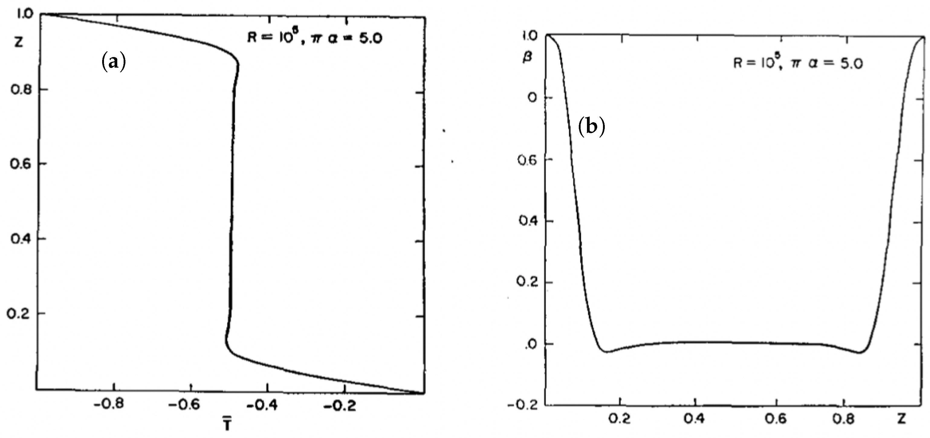
Figure 1.
Rigid (no-slip) boundaries with and . (a) Mean temperature . (b) Mean gradient . has been normalized by the total heat transport . Figure 6a,b from Ref. [2].
Figure 1.
Rigid (no-slip) boundaries with and . (a) Mean temperature . (b) Mean gradient . has been normalized by the total heat transport . Figure 6a,b from Ref. [2].

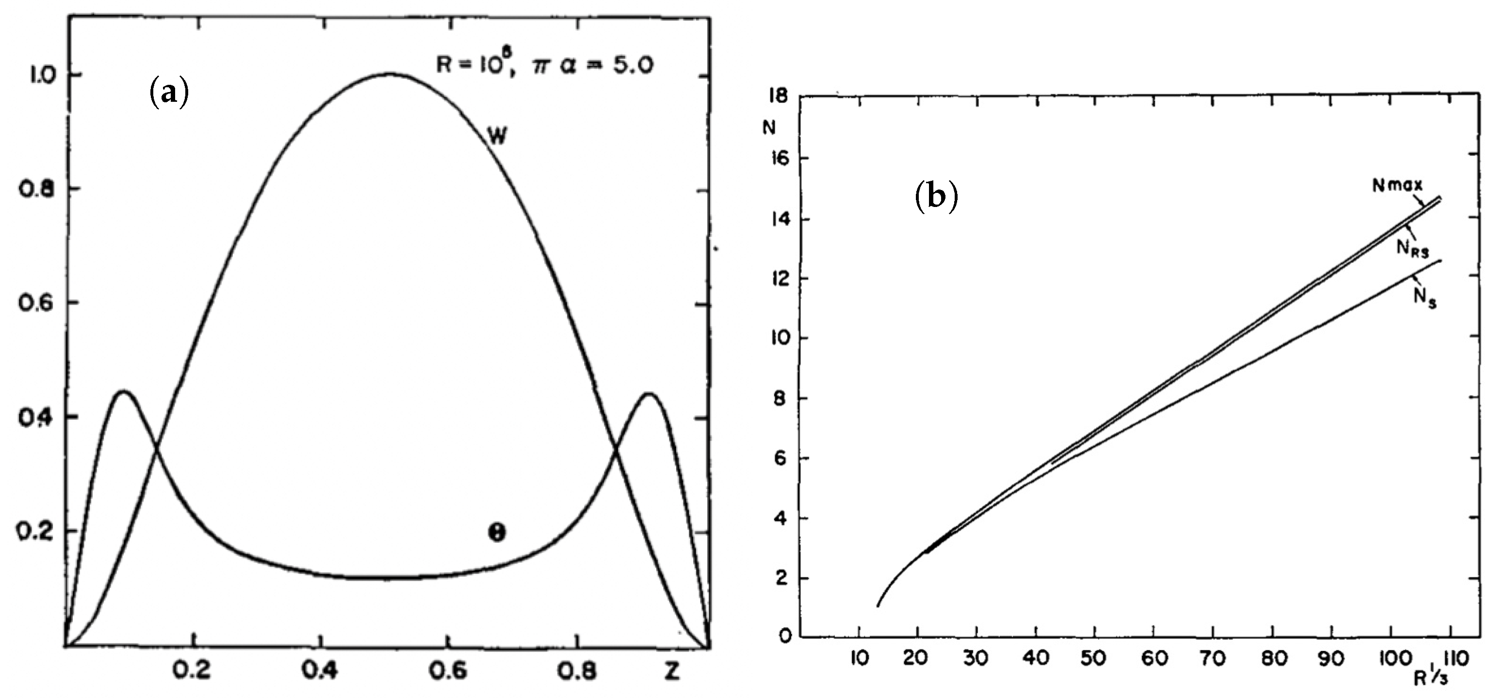
Figure 2.
(a) and for and . (b) The heat flux as a function of from three estimates: is the maximum value of (over different ) for each given . is the flux predicted by the relative stability criterion, and is the heat transported by stable single- solutions. The coefficient given in the abstract is . Figures 5 and 12 from Ref. [2].

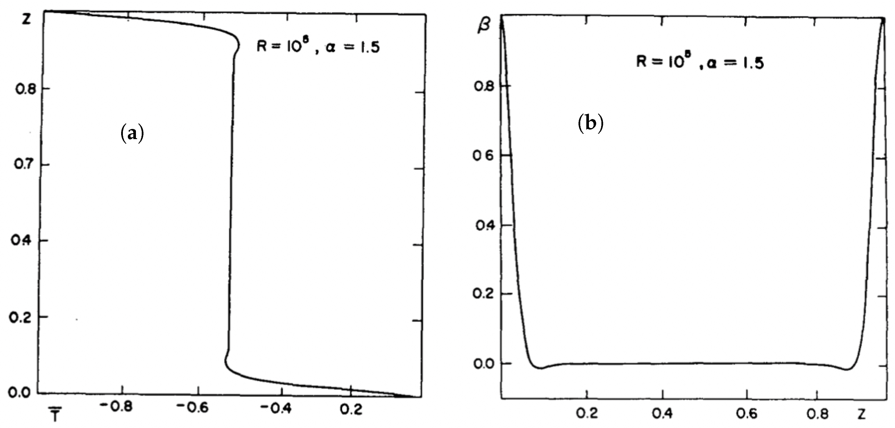
Figure 3.
h-slip with and . (a) Mean temperature . (b) Mean gradient . has been normalized by the total heat transport . Figure 7 from Ref. [1].
Figure 3.
h-slip with and . (a) Mean temperature . (b) Mean gradient . has been normalized by the total heat transport . Figure 7 from Ref. [1].

Figure 4.
(a) and for and . (b) Maximum total heat flux as a function of . Figures 6 and 16 from Ref. [1].
Figure 4.
(a) and for and . (b) Maximum total heat flux as a function of . Figures 6 and 16 from Ref. [1].

Disclaimer/Publisher’s Note: The statements, opinions and data contained in all publications are solely those of the individual author(s) and contributor(s) and not of MDPI and/or the editor(s). MDPI and/or the editor(s) disclaim responsibility for any injury to people or property resulting from any ideas, methods, instructions or products referred to in the content. |
© 2023 by the author. Licensee MDPI, Basel, Switzerland. This article is an open access article distributed under the terms and conditions of the Creative Commons Attribution (CC BY) license (https://creativecommons.org/licenses/by/4.0/).
Share and Cite
MDPI and ACS Style
Kerr, R.M. Review of Jackson Herring’s Early Work on Thermal Convection. Atmosphere 2023, 14, 907. https://doi.org/10.3390/atmos14060907
AMA Style
Kerr RM. Review of Jackson Herring’s Early Work on Thermal Convection. Atmosphere. 2023; 14(6):907. https://doi.org/10.3390/atmos14060907
Chicago/Turabian StyleKerr, Robert M. 2023. "Review of Jackson Herring’s Early Work on Thermal Convection" Atmosphere 14, no. 6: 907. https://doi.org/10.3390/atmos14060907
Note that from the first issue of 2016, this journal uses article numbers instead of page numbers. See further details here.