Article

Potential Vorticity Generation in Breaking Gravity Waves

by
Michael L. Waite
* and
Nicholas Richardson
Department of Applied Mathematics, University of Waterloo, Waterloo, ON N2L 3G1, Canada
*
Author to whom correspondence should be addressed.
Current address: Department of Mathematics, University of British Columbia, Vancouver, BC V6T 1Z2, Canada.
Atmosphere 2023, 14(5), 881; https://doi.org/10.3390/atmos14050881
Submission received: 18 April 2023 / Revised: 9 May 2023 / Accepted: 12 May 2023 / Published: 18 May 2023

Abstract

:
Potential vorticity (PV) is an important quantity in stratified flows because it is conserved following the flow in the absence of forcing and viscous and diffusive effects. However, as shown by previous work for unstratified turbulence, viscosity and diffusion, when present, are not purely dissipative and can create potential vorticity even when none is present initially. In this work, we use direct numerical simulations to investigate the viscous and diffusive generation of potential vorticity and potential enstrophy (integrated square PV) in stratified turbulence. Simulations are initialized with a two-dimensional standing internal gravity wave, which has no potential vorticity apart from some low-level random noise; as a result, all potential vorticity and enstrophy comes from viscous and diffusive effects. Significant potential enstrophy is found when the standing wave breaks, and the maximum potential enstrophy increases with increasing Reynolds number. The mechanism for the initial PV generation is spanwise diffusion of buoyancy perturbations, which grow as the standing wave three-dimensionalizes, into the direction of spanwise vorticity. The viscous and diffusive terms responsible are small-scale and are sensitive to under-resolution, so high resolution is required to obtain robust results.

1. Introduction

The Ertel potential vorticity (PV) is an important quantity in geophysical fluid dynamics. PV characterizes the component of vorticity normal to the isosurfaces of a conserved scalar, and it is materially conserved in the absence of forcing and molecular viscosity and diffusion. In quasi-geostrophic (QG) dynamics, where the PV can be inverted to find the velocity and buoyancy, conservation of PV is everything. Even for the primitive dynamics of the atmosphere and ocean, where large-scale QG turbulence interacts with inertia–gravity waves, weakly rotating stratified turbulence at intermediate scales, and isotropic turbulence at small scales, PV is a useful quantity for analyzing the vortical part of the flow. Indeed, PV is the basis of various decomposition methods for separating slow, quasi-horizontal vortical motion, which has PV, from fast, propagating inertia–gravity waves, which have no PV [1,2,3,4].
QG dynamics break down at intermediate length scales in the atmosphere and ocean, where stratification is strong but rotation is weaker than at large scales. Stratified turbulence is often used as an idealization of turbulent dynamics at these scales [5,6]. In stratified turbulence, PV is a useful diagnostic for quantifying the role of vortices and gravity waves. In the Craya–Herring decomposition [7] and the closely related vortical/wave mode decomposition [2], the vortical component of the flow accounts for the linear PV. Lilly [5] proposed that conservation of linear PV might constrain stratified turbulence and lead to an inverse energy cascade, as in two-dimensional turbulence. However, an inverse cascade does not occur in stratified turbulence [6,8], due to a leakage of energy from vortices to gravity waves [9] and the importance of nonlinear terms in the PV [10,11] due to the development of small vertical scales [6,12]. Nevertheless, the question of whether the downscale cascade of energy through such scales in the atmosphere and ocean is dominated by vortices or waves has not yet been fully resolved [13,14].
Since PV is used to diagnose and separate vortices and gravity waves in geophysical flows and stratified turbulence, it is important to know where PV comes from. In QG turbulence, the integrated square PV, called potential enstrophy, cascades conservatively to smaller scales, analogously to the enstrophy cascade in two-dimensional turbulence. As a result, the QG enstrophy cascade from the large-scale circulation is one source of PV at intermediate and small scales in the atmosphere and ocean, where QG breaks down and stratified turbulence may be present.
However, viscosity and diffusion can also create PV. Because PV depends nonlinearly on vorticity and buoyancy, viscous and diffusive effects are not purely dissipative or necessarily restricted to small length scales, as they are for regular vorticity. This effect was explored in unstratified turbulence with a passive scalar by Herring, Kerr, and Rotunno [15]. By analyzing the evolution of PV in decaying turbulence, they found that viscous and diffusive effects on PV may occur at large scales. By considering a Taylor–Green vortex oriented with zero initial PV, they demonstrated that viscosity and diffusion can create large-scale PV even when none is initially present. These findings raised doubts about whether the notion of a potential enstrophy cascade is meaningful in the absence of QG turbulence. Subsequent work suggested that a potential enstrophy cascade may be possible in certain parameter regimes of geophysical turbulence [16], but the role of viscous and diffusive generation of potential vorticity in stratified turbulence has not been explored.
In this paper, inspired by [15], we use direct numerical simulation (DNS) to investigate the role of viscosity and diffusion on the evolution of PV in stratified turbulence. Compared to [15], we explore the effects of stratification and the impact of larger Reynolds numbers. A two-dimensional standing internal gravity wave is used to initialize simulations of decaying stratified turbulence. A standing wave is a linear solution to the equations of motion, but instabilities and nonlinearities inevitably cause the wave to break down into smaller-scale turbulence. Standing waves have been used in laboratory [17] and numerical [18,19,20] studies of stratified turbulence. More generally, numerical simulation is an important tool for studying breaking gravity waves, which are a key source of turbulence in the atmosphere [21,22,23]. A breaking standing wave is a useful flow configuration for quantifying the viscous generation of PV because, like the Taylor–Green case in [15], the initial wave has no PV. As a result, any PV in the resulting turbulence must come from viscous generation. We will explore the magnitude and mechanisms of PV generation, the associated length scales, and the dependence on viscosity and stratification.

2. Materials and Methods

2.1. Equations

We use the uniformly stratified, non-rotating Boussinesq equations to describe stratified turbulence. The equations of motion are
D u D t = p + b z ^ + ν 2 u ,
· u = 0 ,
D b D t + N 2 w = κ 2 b ,
where D / D t = / t + u · is the material derivative, u = ( u , v , w ) is the velocity, b is the buoyancy, p is the pressure scaled by a reference density, N is the constant buoyancy frequency, ν is the kinematic viscosity, κ is the buoyancy diffusivity, and z ^ is the vertical unit vector. There is no forcing. The buoyancy b is proportional to the negative fluctuation of density from the linear basic state, and N 2 is proportional to the background density gradient; the total buoyancy b tot = N 2 z + b is proportional to the (negative) density.
The Ertel PV for (1)–(3) is
q = ω · N 2 z ^ + b = N 2 ω z + ω · b ,
where ω = × u = ( ω x , ω y , ω z ) is the vorticity [24]. The PV evolves according to
D q D t = ν N 2 z ^ + b · 2 ω + κ ω · 2 b = ν N 2 2 ω z + ν b · 2 ω + κ ω · 2 b .
In the absence of viscosity and diffusion, D q / D t = 0 and the PV is materially conserved. When ν , κ > 0 , the evolution of q is more complicated. Due to the nonlinear dependence of q on ω and b, the viscous and diffusive terms in the q Equation (5) are not simply diffusive. Viscous effects can modify q by viscous diffusion of the vorticity into the direction of the buoyancy gradient, either by diffusion of ω z along the background buoyancy gradient N 2 or by diffusion of ω in the direction of b . In addition, buoyancy diffusion can modify q by diffusion of the buoyancy gradient into the direction of the vorticity. As a result, as indicated by [15], viscosity and diffusion may create PV even when none is initially present.
The potential enstrophy is the integrated square PV, and is given by
V = 1 2 q 2 ,
= 1 2 N 4 ω z 2 + N 2 ω z ω · b + 1 2 ω · b 2 ,
where · denotes domain average. Assuming no flux through the boundary, the potential enstrophy satisfies
d V d t = ν N 2 q 2 ω z + ν q b · 2 ω + κ q ω · 2 b = D ν + D κ ,
where D ν is the term with viscosity ν and D κ is the term with buoyancy diffusivity κ . The viscous and diffusive terms are not necessarily dissipative, and may be a source or sink of potential enstrophy.

2.2. Scale Analysis

We can estimate the magnitude of the potential enstrophy in stratified turbulence using scale analysis. In stratified turbulence with large buoyancy Reynolds number R e b = ϵ / ( ν N 2 ) , where ϵ is the kinetic energy dissipation rate, there should be a Kolmogorov inertial range at small scales between the Ozmidov and Kolmogorov scales
L O = ϵ N 3 1 / 2 , η = ν 3 ϵ 1 / 4 ,
respectively [25,26,27], since L O / η ( R e b ) 3 / 4 [28,29]. Since the PV is a function of the velocity and buoyancy gradients, it should be dominated by the smallest scales when such an inertial range is present.
Consider the third term in (7), which is likely to be the largest term when the Reynolds number is large since it depends on the squared vorticity and squared buoyancy gradient. Using Kolmogorov scaling gives ω υ / η , where υ = ( ν ϵ ) 1 / 4 is the Kolmogorov velocity scale. We assume that the small-scale buoyancy fluctuations are b υ N . As a result, estimating V using the third term in (7) gives
V N 2 ϵ 2 ν 2 N 4 U 2 L 2 R e 2 F r 2 N 4 U 2 L 2 R e b R e ,
where the second and third ∼ use Taylor’s hypothesis ϵ U 3 / L [6], U and L are the large-scale velocity and length scales, R e = U L / ν is the Reynolds number, and F r = U / ( N L ) is the Froude number. Note that N 4 U 2 / L 2 is the magnitude of the potential enstrophy from the large energy-containing scales. This estimate suggests that stratified turbulence may have significant potential enstrophy at small scales, and that potential enstrophy increases with increasing R e and R e b .

2.3. Numerical Approach

Simulations are performed in a cubic domain with size 2 π and periodic boundary conditions. The initial conditions for a two-dimensional standing wave with unit wavenumber, following [19], are
u = a sin x cos z ,
w = a cos x sin z ,
b = 0 ,
where a > 0 is the amplitude and v = 0 . In the linear equations, these initial conditions excite a standing wave
u = a sin x cos z cos ( ω t ) ,
w = a cos x sin z cos ( ω t ) ,
b = a N 2 ω cos x sin z sin ( ω t ) ,
with frequency ω = N / 2 . Since the initial buoyancy and vertical vorticity are zero, the initial standing wave has no PV. Standing waves eventually break and generate small-scale turbulence [19,20]. In particular, the standing wave (14)–(16) is overturning and subject to convective instability when 2 a / N > 1 . In our simulations, the wave amplitude is fixed at a = 1 . Stratification and the overturning of the standing wave are controlled by varying N.
Equations (1)–(3) are simulated with a Fourier-based spectral transform model. Time-stepping is third-order Adams–Bashforth and the viscous and diffusion terms are handled with a Crank–Nicolson approach [30]. Aliasing is removed using the two-thirds rule, so with n 3 grid points, wave vectors k = ( k x , k y , k z ) are truncated at | k x | , | k y | , | k z | = k T = n / 3 , i.e., we keep n / 3 < k x , k y , k z < n / 3 . The resolution n is chosen to resolve the Kolmogorov scale with η k T 2.5 , where η is calculated using the maximum value of ϵ = ν | ω | 2 . As discussed below, high resolution is required to resolve the viscous terms in the q equation properly. While recent studies have shown that stratified turbulence may be sensitive to increasing Prandtl number P r = ν / κ at R e -values that are attainable in DNS [31,32], in this work we set P r = 1 for computational efficiency, so κ = ν . A small amount of random noise is added to the initial velocity, with uniform distribution and magnitude a / 100 , to facilitate three-dimensionalization. This noise introduces a small amount of initial q and V that is quickly removed by viscous and diffusion terms, as shown below.
Since the initial standing wave has unit velocity and unit wavenumber, Equations (1)–(3) can be interpreted as dimensionless with ν = 1 / R e , N = 1 / F r , and unit turnover time. We use ν , N and R e , F r interchangeably in what follows to distinguish stratification and viscosity. Several simulations at different R e and F r are discussed below and summarized in Table 1. The control simulation (Main) has n = 1024 , N = 1 ( F r = 1 ), ν = 0.0003 ( R e = 3333 ), and 2 a / N = 2 , so the standing wave overturns and quickly breaks down into stratified turbulence. Sensitivity to Reynolds number is explored in simulations High Visc and Low Visc, in which R e is decreased to 1667 and increased to 4500. Sensitivity to stratification is explored in simulations High Strat and Higher Strat, in which F r is reduced to 1 / 2 and 1 / 2 . Finally, sensitivity to resolution is investigated in simulations Low Res and High Res by reducing and increasing the resolution to 512 and 1536 grid points.

3. Results

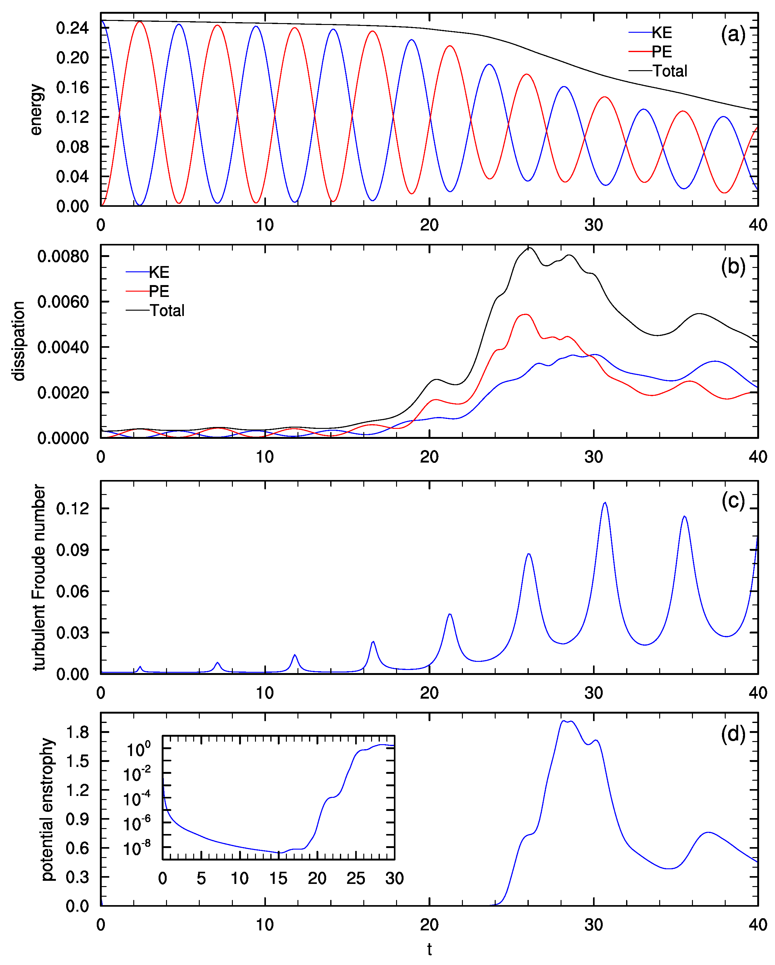
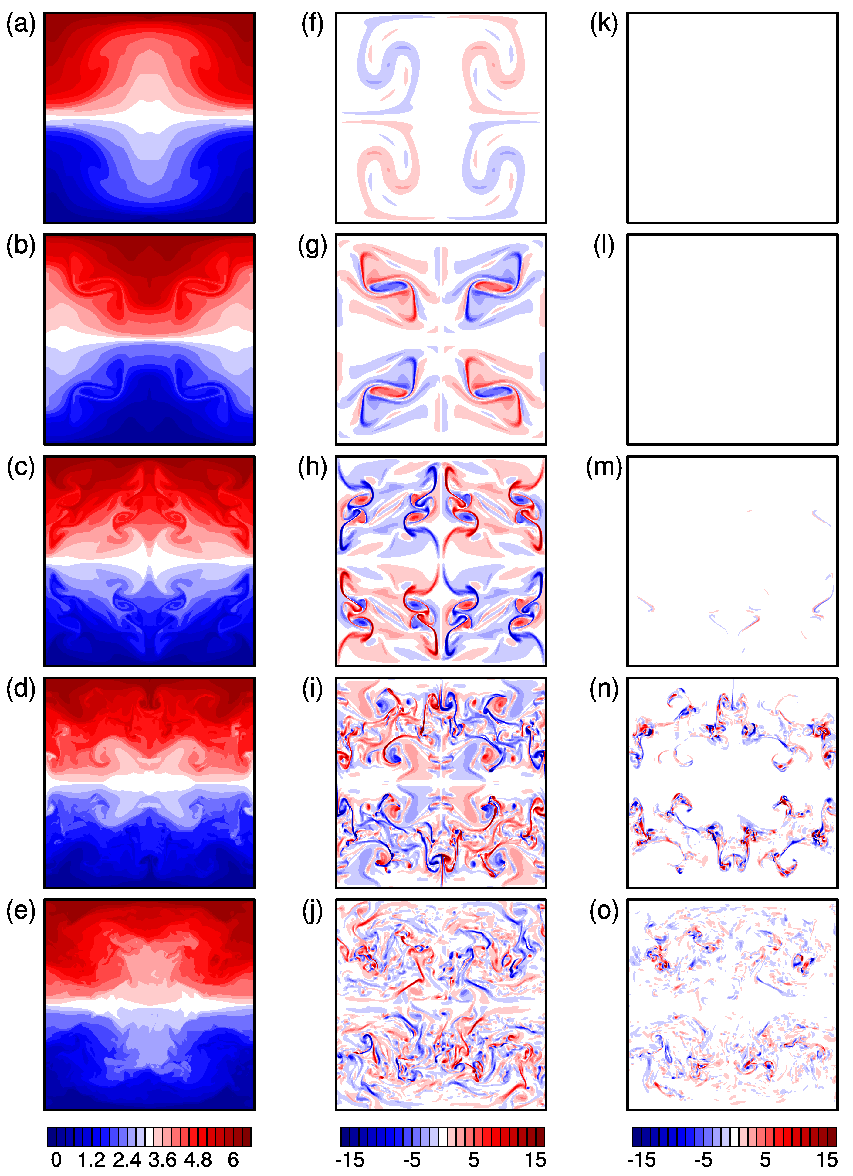
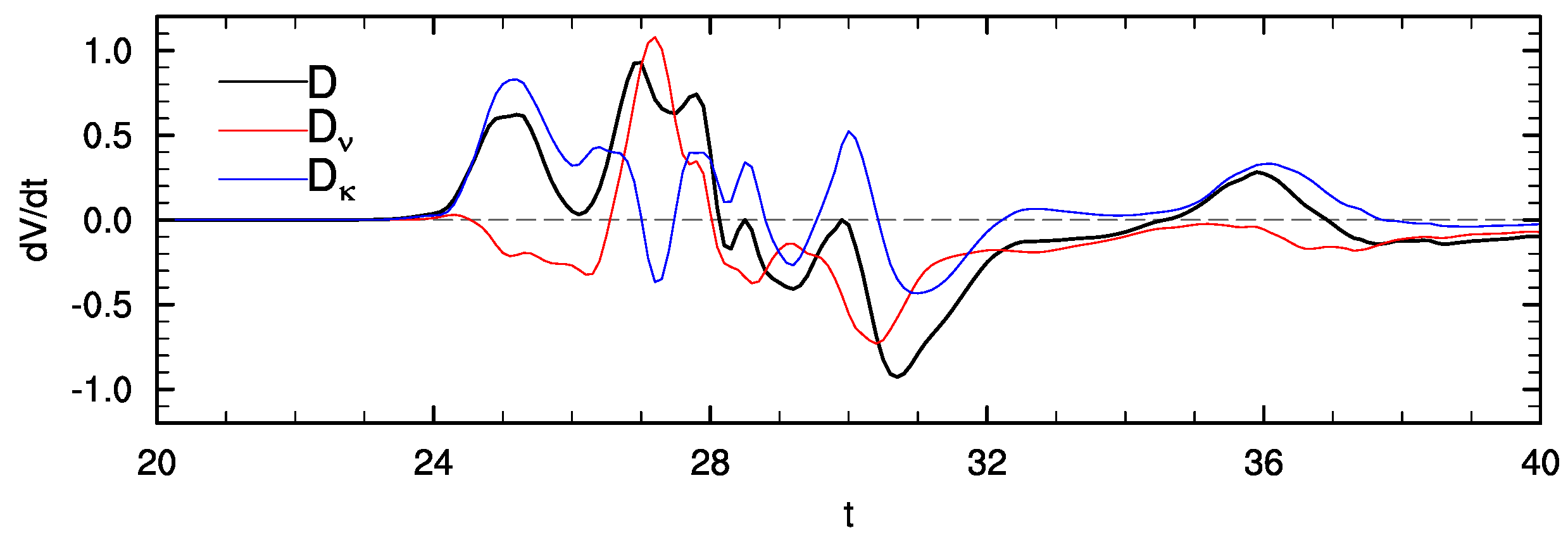
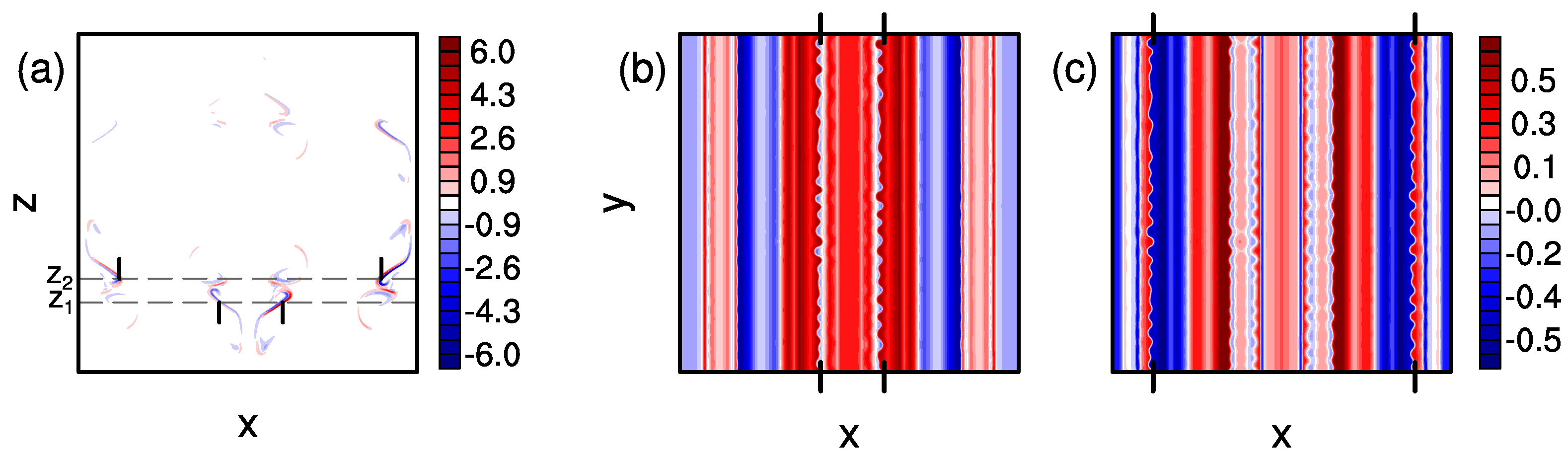
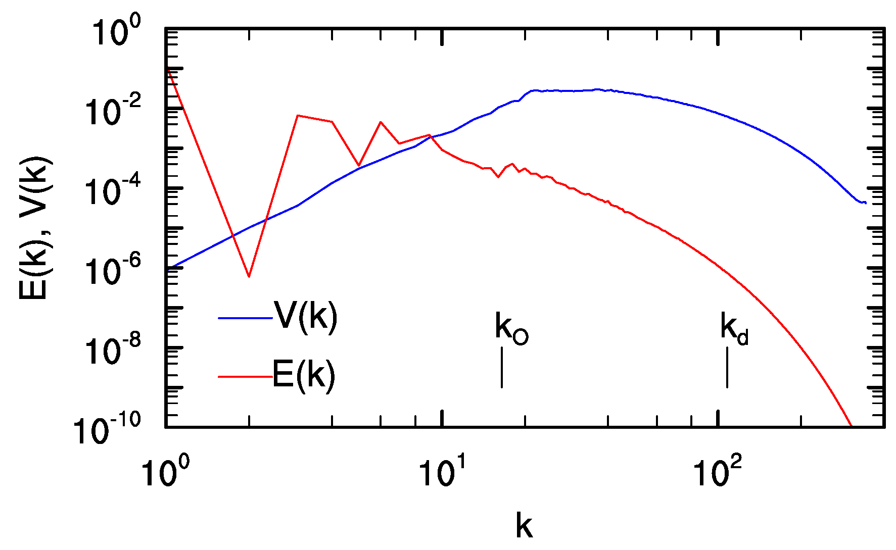
3.1. Main Simulation

We begin by examining the potential enstrophy evolution in the Main simulation, which has F r = 1 , R e = 3333 , and a large, overturning wave amplitude. Time series of kinetic and potential energy, energy dissipation, turbulent Froude number, and potential enstrophy are shown in Figure 1. The wave period for this simulation is T = 2 π 2 8.9 . The wave makes two periods with negligible dissipation. By t = 20 , the energy dissipation begins increasing and the energy begins to decrease more significantly. The potential energy dissipation reaches a maximum at t = 26 , followed by the maximum kinetic energy dissipation at t = 30 . Table 1 gives η k T = 3.2 and R e b = 12.2 , both of which are based on the maximum value of ϵ in the simulation, which is also given in Table 1. Figure 1c shows that the turbulent Froude number F r t = ϵ / ( N E K ) 0.1 , where F r t is defined using velocity scale E K , where E k is the domain-averaged kinetic energy, and length scale from Taylor’s hypothesis [29].
The potential enstrophy in this simulation is shown in Figure 1d. The potential enstrophy is negligible until t 24 . The inset shows V at early times with a log scale; the small potential enstrophy introduced by the random noise decays rapidly until t 15 , and then begins to increase. A maximum value of V = 1.9 is reached at t = 29 . To put this number in perspective, we can calculate the potential enstrophy that would be associated with the initial velocity field if it was rotated by 90 :
V 0 = 1 2 N 4 ω y 0 2 = 1 2 ,
where ω y 0 is the vorticity associated with (11)–(13). Therefore, we can see that significant potential enstrophy is generated in this simulation, about four times larger than what one would expect from the initial velocity field and stratification alone.
Vertical ( x , z ) slices of the total buoyancy b tot , normal component of vorticity ω y , and potential vorticity q are plotted in Figure 2 for a selection of times from t = 16 , before the onset of significant dissipation, to t = 36 , when the turbulence is decaying. First, we discuss the evolution of the buoyancy and normal vorticity (left and centre columns of Figure 2). At t = 16 , the buoyancy (Figure 2a) shows the structure of the standing wave with some overturning isopycnals, as expected. At t = 20 , the overturning isopycnals have collapsed (Figure 2b) with significant spanwise vorticity in the overturning regions (Figure 2g). By t = 24 , the buoyancy field of the standing wave has been significantly altered by breaking (Figure 2c), and smaller spanwise vortices are present (Figure 2h). At t = 28 and 36, the wave has largely broken down into turbulence, with the vorticity dominated by small scales (Figure 2d–e,i–j).
The potential vorticity is shown in the right column of Figure 2. There is no significant PV visible until t = 24 . At t = 24 , thin bands of positive and negative PV appear, mainly in the lower overturning region (similar bands are apparent in the upper overturning region at other y). By t = 28 , the PV structure has become more rich and complex, with both small-scale bands and vortex structures visible. At this time, the PV is still mainly located in the upper and lower breaking regions, avoiding z = 0 , π , and 2 π . This time corresponds to the maximum V in Figure 1d. The PV occupies more of the domain at t = 36 , but the amplitude is lower, consistent with the decay of V seen in Figure 1d.
To investigate the increase in PV around t 24 , time series of the terms in the potential enstrophy Equation (8) are shown in Figure 3. These terms are negligible for t 24 , but begin to deviate from zero for t 24 . From 24 < t < 26 , the buoyancy diffusivity term D κ dominates, and is responsible for the initial creation of V as the wave begins to break. At these times, the viscous terms are slightly dissipative. V grows rapidly from 24 < t < 26 , but the growth slows around t = 26 (Figure 1d). At t = 26 , the growth in V increases again, this time, as seen in Figure 3, due to a sharp increase in the viscous term D ν . After around t = 28 , the combined viscous and diffusion term is negative and V decreases, apart from a short increase in V around t = 36 .
Figure 3 indicates that the initial generation of PV, as seen in the rise in V, is a result of the κ term in the V equation, which corresponds to diffusion of the buoyancy gradient into the direction of vorticity. The κ term can be decomposed as
D κ = κ q ω · 2 ( b ) = κ q ω x 2 b x + κ q ω y 2 b y + κ q ω z 2 b z .
For 24 < t < 26 , D κ is dominated by the second term, which involves ω y and b / y (not shown). The mechanism of PV generation by this term is illustrated in Figure 4, which shows a vertical slice of q and two horizontal slices of b at t = 24 . The flow is still mainly two-dimensional at this time, but three-dimensionalization of the buoyancy field is visible along a few lines parallel to the y-axis in Figure 4b,c. The planes z = z 1 and z = z 2 cut through bands of PV in the lower breaking region. Along z 1 , the PV bands occur precisely where the buoyancy field is three-dimensionalizing, as seen in Figure 4b, where the ticks mark the locations of the PV along z 1 in Figure 4a. Similarly, the PV bands along z = z 2 occur at the same location as the buoyancy three-dimensionalization at that height. Three-dimensionalization of b promotes growth of b / y , which diffuses into the direction of ω y , which at this time is still the dominant component of the vorticity. Therefore, PV first emerges at the locations where three-dimensionalization of the buoyancy develops, via the second term in (18).
Kinetic energy spectra E ( k ) and potential enstrophy spectra V ( k ) , plotted as functions of the total wavenumber k = | k | , are shown in Figure 5. Spectra are calculated at t = 28 , which is the time of maximum potential enstrophy. As expected, the energy spectrum is peaked at the primary standing wave wavenumber k = 1 , oscillates at the lowest few wavenumbers, and then falls off like a power law until the Kolmogorov wavenumber, which is marked in the figure. By contrast, the potential enstrophy spectrum is peaked at large wavenumbers. It has a positive slope of around 3.3 for 1 k 20 . Despite the fact that V is generated by viscous and diffusive effects, V ( k ) has a broad peak around k 20 to 40, which is just beyond the Ozmidov wavenumber, which is marked in the figure. However, we will see below that this peak is not set by the Ozmidov wavenumber.

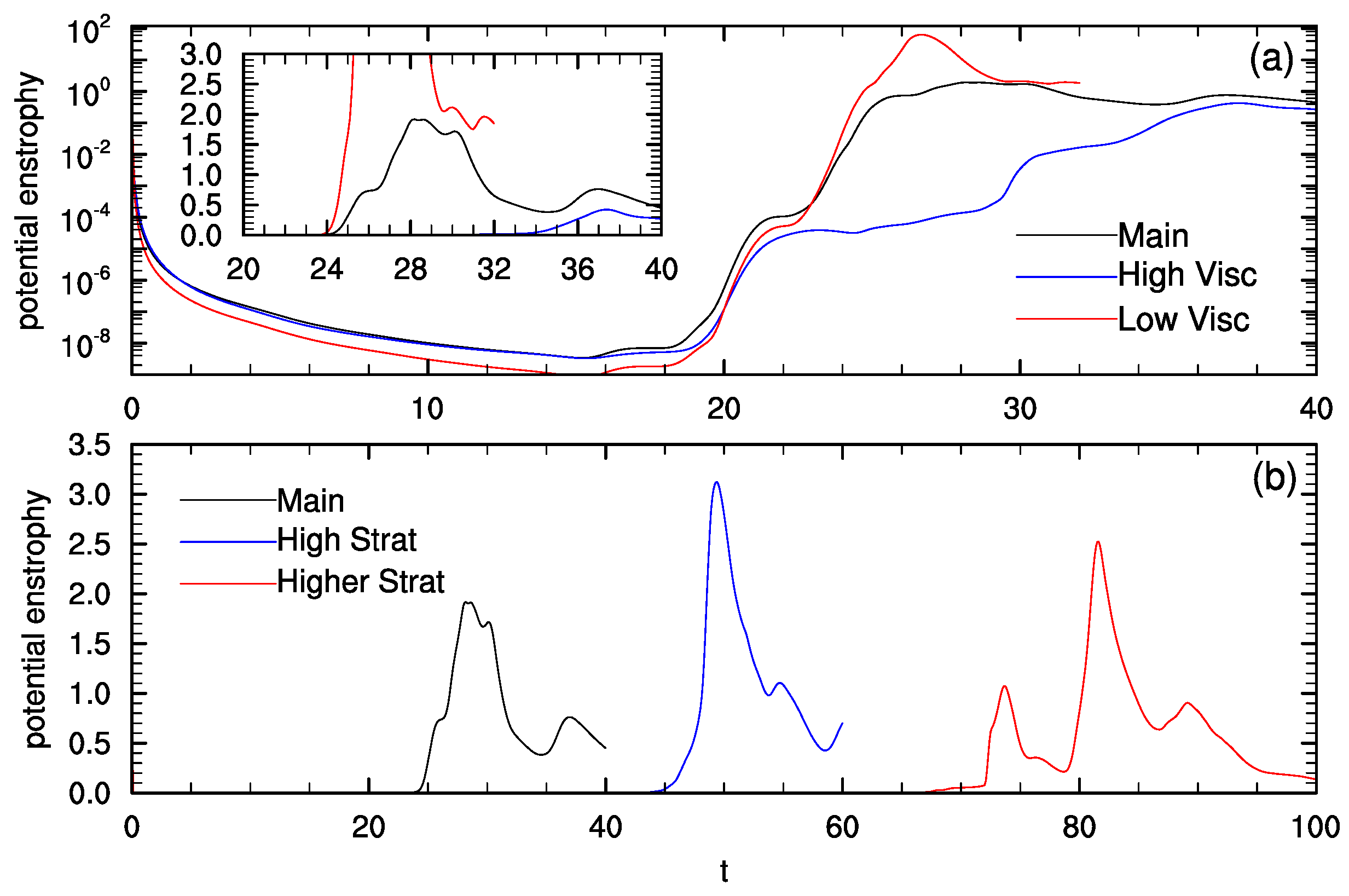
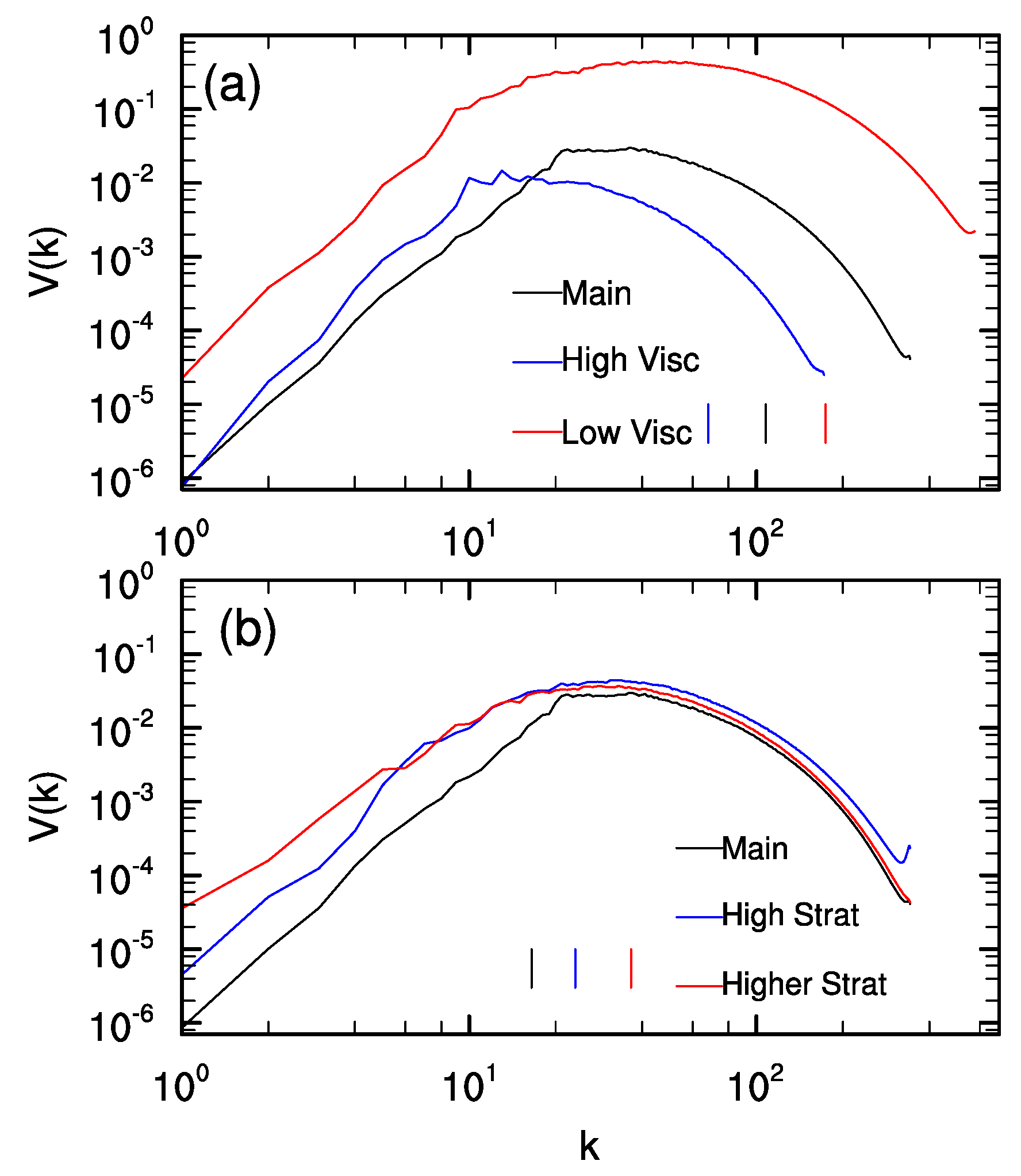
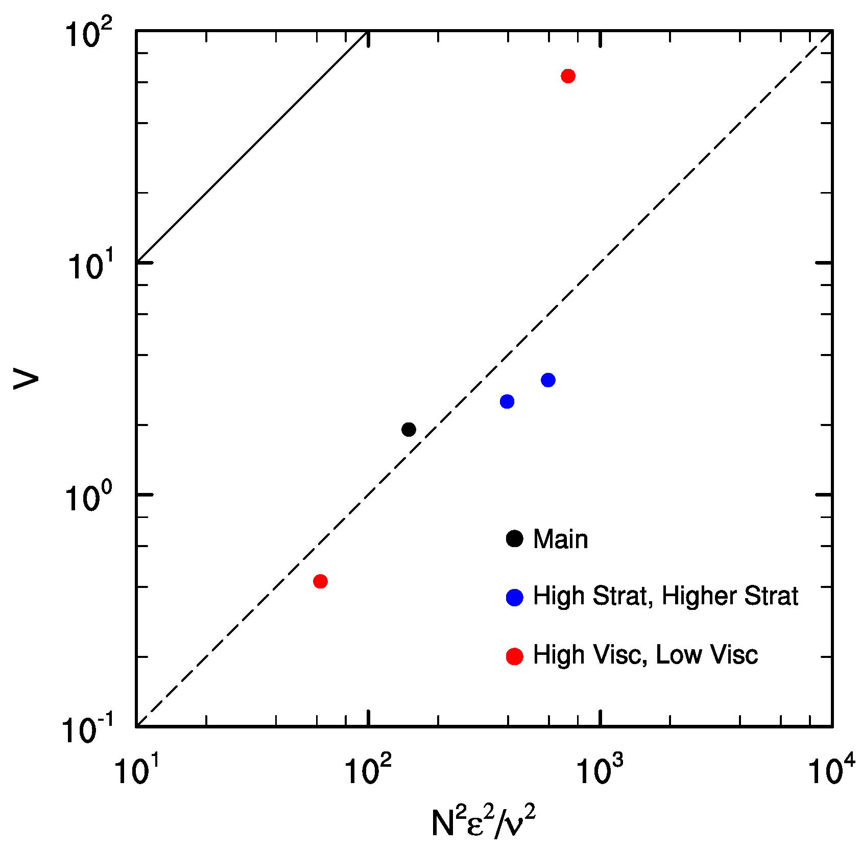
3.2. Sensitivity to Reynolds and Froude Numbers

We investigate the dependence of viscous and diffusive PV generation on Reynolds number with two additional simulations with lower and higher Reynolds numbers. The Reynolds number is varied by changing ν , and the resolution is adjusted to resolve the Kolmogorov scale. Time series of the potential enstrophy for these simulations, along with the Main simulation, are shown in Figure 6a. With smaller R e , the maximum potential enstrophy is reduced from around 1.9 to 0.4. The time of maximum potential enstrophy is also delayed, from around t = 28 in the Main simulation to t = 37 in the High Visc simulation. On the other hand, for the Low Visc simulation with larger R e , the maximum potential enstrophy is much larger, reaching a value of around 64 at t = 27 , which is slightly earlier than the Main simulation. Potential enstrophy spectra from these simulations are shown in Figure 7a. The potential enstrophy spectra for the Main and High Visc experiments are similar at small k but increase with increasing R e at larger k, indicating that the increased potential enstrophy with higher Reynolds number is primarily at small scales going from High Visc to Main. However, the potential enstrophy in the Low Visc case is increased at all scales, not just small scales.
Time series of potential enstrophy from simulations with increased stratification are shown in Figure 6b. Increasing the stratification delays the onset of wave breaking and, as a result, the growth in potential enstrophy is also delayed. The High Strat simulation has 2 a / N = 1 and is therefore on the threshold of convective instability; this simulation reaches a maximum potential enstrophy of 3.1 at t = 49 , which is larger and later than in the Main simulation. The Higher Strat simulation has 2 a / N = 1 / 2 and reaches a maximum V of 2.5 at t = 82 . This is a smaller maximum V than in the High Strat simulation, and it also occurs later. Potential enstrophy spectra from these simulations are shown in Figure 7b. The peak in potential enstrophy remains around k 20 to 40, even as the Ozmidov wavenumber, which is shown in the figure, increases from 16 to 37 with increasing stratification. The peak in the potential enstrophy spectrum therefore does not scale with the Ozmidov wavenumber. In addition, the large-scale potential enstrophy, with k < 20 , increases with increasing stratification.
To make sense of the dependence of V on viscosity and stratification, we can compare our simulation results with the prediction (10). The dependence on stratification in particular is difficult to understand, because the maximum V seems to increase, then decrease, with increasing stratification. However, analyzing the dependence of V on F r or N alone presents an incomplete picture, because the strength of the turbulence, as captured by the maximum ϵ , also changes with stratification (Table 1). Equation (10) suggests that the maximum V should depend on ν , N, and ϵ . Figure 8 shows the maximum V plotted against N 2 ϵ 2 / ν 2 , where the maximum value of ϵ is used (maximum ϵ generally occurs around the same time as maximum V). While the agreement with (10) is not particularly good, we do find that maximum V increases with increasing N 2 ϵ 2 / ν 2 , which accounts for the non-monotonic dependence on stratification. In all cases, the maximum potential enstrophy is less than what was predicted by (10), but the Low Visc case, which has the highest R e and R e b , is closest to (10).

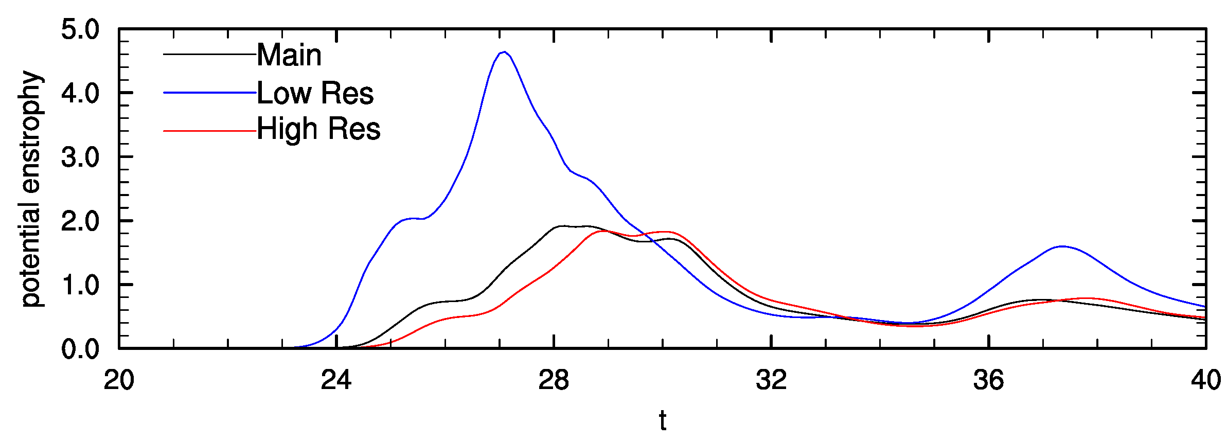
3.3. Sensitivity to Numerical Resolution

High spatial resolution is required to accurately resolve the viscous and diffusive terms in the PV equation. Under-resolution can lead to spurious generation of PV. The dependence on resolution is illustrated in Figure 9, which shows time series of V for the Main simulation and simulations with higher and lower resolution. The Low Res simulation, which has η k T = 1.5 , has a maximum V of around 4.6. This value is more than double the maximum V of 1.9 in the Main simulation, which has η k T = 3.2 . By contrast, the High Res simulation, which has η k T = 4.6 , has a maximum V of 1.8, which is just slightly smaller than the value in the Main simulation. The timing of maximum V is slightly accelerated in the Main simulation compared to the High Res simulation, but these simulations are much closer to one another than to the Low Res case. Inadequate resolution results in accelerated and artificially high potential enstrophy growth.

4. Discussion

A breaking standing gravity wave is a useful case for studying viscous and diffusive generation of PV in stratified turbulence because such flows have no initial PV. Any PV that develops must come from viscous and diffusive effects. Our simulations indicate that significant PV and potential enstrophy are created as these waves break, much more than would be expected from the velocity and length scales of the breaking wave. Indeed, more potential enstrophy is created at higher Reynolds numbers, because even though the viscosity and diffusion coefficients are smaller, the velocity and buoyancy gradients in the turbulence are correspondingly larger. The Reynolds numbers in this work, while large compared to what was possible in [15], are still small compared to geophysical fluid values. It therefore seems likely that viscous and diffusive generation of PV from breaking gravity waves may be even more significant in the atmosphere and ocean.
The mechanism of the initial PV generation is diffusion of spanwise buoyancy fluctuations, which develop as the waves three-dimensionalize, into the direction of the spanwise vorticity, which is initially dominant. As a result, the initial PV generation occurs at small length scales associated with three-dimensionalization of the flow. Once significant potential enstrophy is present, spectra are peaked at intermediate wavenumbers 20–40, corresponding to scales smaller than the wavelength of the breaking wave, but much larger than the Kolmogorov scale. Interestingly, this intermediate scale does not vary like the Ozmidov scale, and indeed does not change much with Reynolds or Froude number, indicating that it might be related to the scale of the breaking wave. The potential enstrophy at large scales, while relatively small, increases with increasing Reynolds numbers and decreasing Froude numbers.
The mechanism of PV generation in breaking standing waves is somewhat different from the Taylor–Green vortices considered by [15]. The Taylor–Green vortices were oriented so that they had no initial PV, like the standing wave. Potential enstrophy in their case was initially created at large scales, followed by more intense generation at small scales; they confirmed that the small-scale generation was due to viscous and diffusive effects rather than transfer from large scales. The standing wave does not have significant large-scale potential enstrophy at early times. However, for both the Taylor–Green vortex in [15] and our standing wave, viscous and diffusive effects are primarily a source of potential enstrophy; dissipation takes over only at late times. By contrast, for the decaying turbulence with Gaussian initial conditions considered in [15], viscous and diffusive effects were primarily dissipative. More work is required to determine if the differences between our results and the pioneering work of [15] are due to the different Reynolds numbers, initial configuration, or the presence of stratification. In addition, it would be interesting to examine the role of viscous and diffusive effects in stratified turbulence with large-scale PV from random initial conditions or forcing.
Viscous and diffusive generation of potential enstrophy is sensitive to numerical resolution. DNS requires resolution of the Kolmogorov scale. Resolutions with η k T 1 are typical for DNS of breaking gravity waves [23] and decaying stratified turbulence [33]. However, our findings show that under-resolution can lead to spurious generation of PV when η k T = 1.5 . Instead, larger values of η k T 2.5 are needed for robust simulations of potential enstrophy generation. Such high resolution is not routinely employed for DNS of stratified turbulence. This finding, while perhaps not surprising given the small-scale mechanisms at play, suggests that some DNS studies of stratified turbulence and gravity wave breaking may have unrealistically high potential enstrophy due to under-resolution of the viscous generation processes. More work is required to understand the implications on the dynamics of turbulence with artificially enhanced potential enstrophy.

Author Contributions

Conceptualization, M.L.W.; methodology, M.L.W.; software, M.L.W. and N.R.; validation, M.L.W. and N.R.; writing—original draft preparation, M.L.W.; writing—review and editing, M.L.W. and N.R.; visualization, M.L.W.; supervision, M.L.W. All authors have read and agreed to the published version of the manuscript.

Funding

This research was funded by the Natural Sciences and Engineering Research Council of Canada grant number RGPIN-07001-2020.

Data Availability Statement

Model data are available upon request to the corresponding author.

Acknowledgments

This research was enabled in part by support provided by Compute Ontario (www.computeontario.ca (accessed on 10 May 2023)) and the Digital Research Alliance of Canada (www.alliancecan.ca (accessed on 10 May 2023)).

Conflicts of Interest

The authors declare no conflict of interest.

References

  1. Staquet, C.; Riley, J.J. On the Velocity Field Associated with Potential Vorticity. Dyn. Atmos. Oceans 1989, 14, 93–123. [Google Scholar] [CrossRef]
  2. Lelong, M.P.; Riley, J.J. Internal Wave-Vortical Mode Interactions in Strongly Stratified Flows. J. Fluid Mech. 1991, 232, 1–19. [Google Scholar] [CrossRef]
  3. Bartello, P. Geostrophic Adjustment and Inverse Cascades in Rotating Stratified Turbulence. J. Atmos. Sci. 1995, 52, 4410–4428. [Google Scholar] [CrossRef]
  4. Kafiabad, H.A.; Bartello, P. Balance Dynamics in Rotating Stratified Turbulence. J. Fluid Mech. 2016, 795, 914–949. [Google Scholar] [CrossRef]
  5. Lilly, D.K. Stratified Turbulence and the Mesoscale Variability of the Atmosphere. J. Atmos. Sci. 1983, 40, 749–761. [Google Scholar] [CrossRef]
  6. Lindborg, E. The Energy Cascade in a Strongly Stratified Fluid. J. Fluid Mech. 2006, 550, 207–242. [Google Scholar] [CrossRef]
  7. Herring, J.R. Approach of Axisymmetric Turbulence to Isotropy. Phys. Fluids 1974, 17, 859–872. [Google Scholar] [CrossRef]
  8. Herring, J.R.; Métais, O. Numerical Experiments in Forced Stably Stratified Turbulence. J. Fluid Mech. 1989, 202, 97–115. [Google Scholar] [CrossRef]
  9. Waite, M.L.; Bartello, P. Stratified Turbulence Dominated by Vortical Motion. J. Fluid Mech. 2004, 517, 281–308. [Google Scholar] [CrossRef]
  10. Waite, M.L. Potential Enstrophy in Stratified Turbulence. J. Fluid Mech. 2013, 722, R4. [Google Scholar] [CrossRef]
  11. Rosenberg, D.; Pouquet, A.; Marino, R. Correlation Between Buoyancy Flux, Dissipation and Potential Vorticity in Rotating Stratified Turbulence. Atmosphere 2021, 12, 157. [Google Scholar] [CrossRef]
  12. Billant, P.; Chomaz, J.M. Self-Similarity of Strongly Stratified Inviscid Flows. Phys. Fluids 2001, 13, 1645–1651. [Google Scholar] [CrossRef]
  13. Callies, J.; Bühler, O.; Ferrari, R. The Dynamics of Mesoscale Winds in the Upper Troposphere and Lower Stratosphere. J. Atmos. Sci. 2016, 73, 4853–4872. [Google Scholar] [CrossRef]
  14. Li, Q.; Lindborg, E. Weakly or Strongly Nonlinear Mesoscale Dynamics Close to the Tropopause. J. Atmos. Sci. 2018, 75, 1215–1229. [Google Scholar] [CrossRef]
  15. Herring, J.R.; Kerr, R.M.; Rotunno, R. Ertel’s Potential Vorticity in Unstratified Turbulence. J. Atmos. Sci. 1994, 51, 35–47. [Google Scholar] [CrossRef]
  16. Kurien, S.; Smith, L.; Wingate, B. On the two-point correlation of potential vorticity in rotating and stratified turbulence. J. Fluid Mech. 2006, 555, 131–140. [Google Scholar] [CrossRef]
  17. Benielli, D.; Sommeria, J. Excitation of Internal Waves and Stratified Turbulence by Parametric Instability. Dyn. Atmos. Oceans 1996, 23, 335–343. [Google Scholar] [CrossRef]
  18. Bouruet-Aubertot, P.; Sommeria, J.; Staquet, C. Breaking of Standing Internal Gravity Waves Through Two-Dimensional Instabilities. J. Fluid Mech. 1995, 285, 265–301. [Google Scholar] [CrossRef]
  19. Bouruet-Aubertot, P.; Sommeria, J.; Staquet, C. Stratified Turbulence Produced by Internal Wave Breaking: Two-Dimensional Numerical Experiments. Dyn. Atmos. Oceans 1996, 23, 357–369. [Google Scholar] [CrossRef]
  20. Carnevale, G.F.; Briscolini, M.; Orlandi, P. Buoyancy- to Inertial-Range Transition in Forced Stratified Turbulence. J. Fluid Mech. 2001, 427, 205–239. [Google Scholar] [CrossRef]
  21. Fritts, D.C.; Isler, J.R.; Andreassen, Ø. Gravity Wave Breaking in Two and Three Dimensions 2. Three-Dimensional Evolution and Instability Structure. J. Geophys. Res. 1994, 99, 8109–8123. [Google Scholar] [CrossRef]
  22. Dörnbrack, A. Turbulent mixing by breaking gravity waves. J. Fluid Mech. 1998, 375, 113–141. [Google Scholar] [CrossRef]
  23. Remmler, S.; Fruman, M.D.; Hickel, S. Direct Numerical Simulation of a Breaking Inertia-Gravity Wave. J. Fluid Mech. 2013, 722, 424–436. [Google Scholar] [CrossRef]
  24. Pedlosky, J. Geophysical Fluid Dynamics, 2nd ed.; Springer: Berlin, Germany, 1987. [Google Scholar]
  25. Dougherty, J.P. The Anisotropy of Turbulence at the Meteor Level. J. Atmos. Terr. Phys. 1961, 21, 210–213. [Google Scholar] [CrossRef]
  26. Ozmidov, R.V. On the Turbulent Exchange in a Stably Stratified Ocean. Izvestia Akad. Nauk. SSSR Atmospheric and Oceanic Physics Ser. 1965, 1, 853–860. [Google Scholar]
  27. Davidson, P.A. Turbulence in Rotating, Stratified and Electrically Conducting Fluids; Cambridge University Press: Cambridge, UK, 2013. [Google Scholar]
  28. Gargett, A.E.; Osborn, T.R.; Nasmyth, P.W. Local Isotropy and the Decay of Turbulence in a Stratified Fluid. J. Fluid Mech. 1984, 144, 231–280. [Google Scholar] [CrossRef]
  29. Brethouwer, G.; Billant, P.; Lindborg, E.; Chomaz, J.M. Scaling Analysis and Simulation of Strongly Stratified Turbulent Flows. J. Fluid Mech. 2007, 585, 343–368. [Google Scholar] [CrossRef]
  30. Durran, D.R. Numerical Methods for Wave Equations in Geophysical Fluid Dynamics; Springer: Berlin, Germany, 1999. [Google Scholar]
  31. Legaspi, J.D.; Waite, M.L. Prandtl Number Dependence of Stratified Turbulence. J. Fluid Mech. 2020, 903, A12. [Google Scholar] [CrossRef]
  32. Riley, J.J.; Couchman, M.M.P.; de Bruyn Kops, S.M. The Effect of Prandtl Number on Decaying Stratified Turbulence. J. Turbul. 2023, 1–19. [Google Scholar] [CrossRef]
  33. Maffioli, A.; Davidson, P.A. Dynamics of Stratified Turbulence Decaying From a High Buoyancy Reynolds Number. J. Fluid Mech. 2016, 786, 210–233. [Google Scholar] [CrossRef]
Figure 1. Time series from the Main simulation of (a) kinetic and potential energy, (b) kinetic and potential energy dissipation, (c) turbulent Froude number, and (d) potential enstrophy. The inset in (d) shows potential enstrophy on a log scale to illustrate the decay of the initial potential enstrophy from random noise.
Atmosphere 14 00881 g001
Figure 2. Vertical ( x , z ) slices of (ae) b tot , (fj) ω y , and (ko) q at (from top to bottom) t = 16 , 20, 24, 28, and 36 from Main simulation. All slices are shown at y = 0 .
Atmosphere 14 00881 g002
Figure 3. Time series of the terms in the potential enstrophy Equation (8) from the Main simulation.
Atmosphere 14 00881 g003
Figure 4. (a) Vertical ( x , z ) slice of q, and horizontal ( x , y ) slices of b through (b) z = z 1 and (c) z = z 2 , for the Main simulation at t = 24 . Note that z 1 and z 2 are shown in (a). The vertical line segments in (a) mark the locations of significant PV along z = z 1 and z = z 2 ; these locations are marked with ticks in (b) for z 1 and (c) for z 2 , respectively.
Atmosphere 14 00881 g004
Figure 5. Energy and potential enstrophy spectra from the Main simulation at t = 28 . The Ozmidov and Kolmogorov wavenumbers k O = 1 / L O and k d = 1 / η are shown.
Atmosphere 14 00881 g005
Figure 6. Time series of potential enstrophy from simulations with (a) different R e and (b) different F r . A log scale is used in (a) with a linear scale in the inset.
Atmosphere 14 00881 g006
Figure 7. Potential enstrophy spectra from simulations with (a) different R e and (b) different F r , at the time of maximum potential enstrophy. The vertical line segments mark the Kolmogorov wavenumbers in (a) and the Ozmidov wavenumbers in (b).
Atmosphere 14 00881 g007
Figure 8. Maximum potential enstrophy V plotted against N 2 ϵ 2 / ν 2 , where the maximum value of ϵ is used, for the Main simulation (black), simulations with different stratifications (High Strat and Higher Strat, in blue), and simulations with different viscosities (Low Visc and High Visc, in red). The reference lines are V = N 2 ϵ 2 / ν 2 (solid) and V = 0.01 N 2 ϵ 2 / ν 2 (dashed).
Atmosphere 14 00881 g008
Figure 9. Time series of potential enstrophy from simulations with different resolutions.
Atmosphere 14 00881 g009
Table 1. Summary of simulations.
Run Fr 2 a / N Re nMax  ϵ η k T Max Re b
Main1 2 333310240.00373.212.2
High Visc1 2 16675120.00472.57.9
Low Visc1 2 450017280.00603.826.9
High Strat 1 / 2 1333310240.00522.98.6
Higher Strat1/2 1 / 2 333310340.00303.32.5
Low Res1 2 33335120.00411.513.8
High Res1 2 333315360.00404.613.2
Disclaimer/Publisher’s Note: The statements, opinions and data contained in all publications are solely those of the individual author(s) and contributor(s) and not of MDPI and/or the editor(s). MDPI and/or the editor(s) disclaim responsibility for any injury to people or property resulting from any ideas, methods, instructions or products referred to in the content.

