Assessment of Mechanical Draft Cooling Tower Thermal Emissions from Visual Images of Plumes

Abstract

Using a one-dimensional code, we computed the power (enthalpy discharge rate) of a twelve-cell mechanical draft cooling tower (MDCT) using over two hundred visible condensed water vapor plume volume measurements derived from images, weather data, and tower operating conditions. The plume images were simultaneously captured by multiple stationary digital cameras surrounding the cooling tower. An analysis technique combining structure from motion (SfM), a neural-network-based image segmentation algorithm, and space carving was used to quantify the volumes. Afterwards, the power output was computed using novel techniques in the one-dimensional code that included cooling tower exhaust plume adjacency effects implemented with a modified version of the entrainment function, weather data averaged from eleven stations, and fan operations at the times when plume volumes were measured. The model was then compared with the averaged observed power output, and it validated well with an average error ranging from 6 to 12%, depending on the meteorological data used in the simulations. This methodology can possibly determine power plant fuel consumption rates by applying visible imagery.

1. Introduction

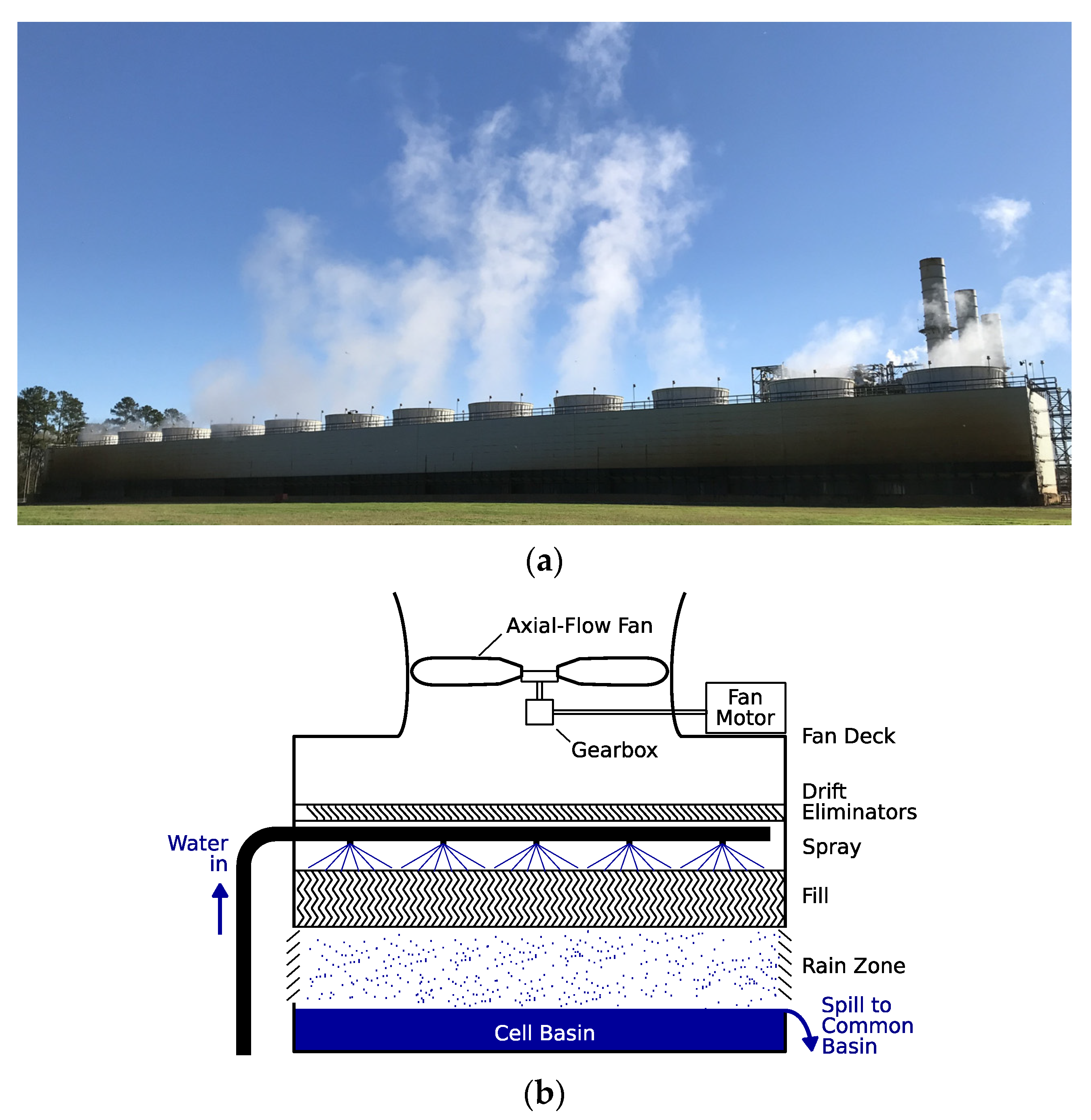
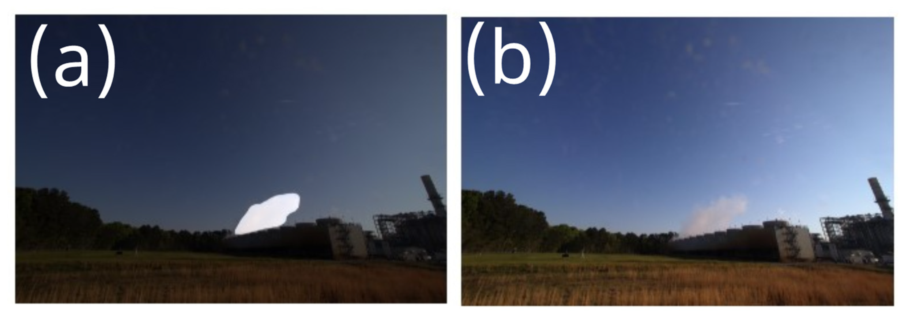
Mechanical draft cooling towers (MDCT) transfer heat from industrial cooling water to the atmosphere via forced convection and evaporation driven by fans. They are typically arranged with multiple independent cells in a row, as seen in Figure 1a. Heated water is sprayed evenly into the top of the fill structure where most of the heat and mass transfer occurs, as illustrated in Figure 1b. The fill structure is made of hard plastic with a honeycomb geometry that optimizes heat and mass transfer from the water to the air. After passing through the fill, the cooling water falls into a common basin from which it returns to the industrial process. Water temperature may be regulated by changing the number of fans operating or, in some facilities, the speed of individual fans. Individual cells can operate in free convection mode (fan off) which reduces the enthalpy transfer rate.

The exhaust created by an MDCT is initially a forced jet which transitions to a buoyant plume higher up. An MDCT operating close to design specifications often produces a visible plume of water droplets that form when the saturated exhaust air mixes with cooler ambient air. Visible MDCT plume droplets grow to only 2 to 3 microns in diameter during their short existence. Drift eliminators prevent large droplets from leaving the tower, so the visible exhaust plume is almost entirely composed of very small droplets that start to form as the exhaust exits the cell. Additional entrainment of sub-saturated ambient air eventually causes the droplets to evaporate. The exhaust plume will continue to rise after all droplets have evaporated until entrainment and expansion in a stable atmosphere eliminate the plume’s buoyancy. The maximum height and volume attained by the visible plume is a strong function of ambient relative humidity, which produces a strong diurnal cycle in plume height. The droplets evaporate almost instantly when entrainment of ambient air causes the relative humidity of the air around the droplet to drop below 100%. For this reason, when the visible plume disappears, the droplets have completely evaporated.

Visible cooling tower plumes and the means of modeling them have been occasionally studied for the purposes of visual impact and the practical impacts of fogging and deposited water in relationship with the enthalpy in the atmosphere. Plume emissions from volcanic eruptions have been measured and quantified to estimate volcanic discharge, analogous to what we propose in this paper [1]. Cizek and Noicka studied how plume volumes were affected by the stack diameters as well as the temperatures of the ambient air and exhaust [2]. Three-dimensional computational fluid dynamics (CFD) studies of cooling tower plumes have appeared in recent literature. CFD modeling has been used to further investigate the plume volume, length, and width with and without a wind velocity, which has also inspired other studies on plume volume flux [3,4,5,6]. Takata et al. used a Reynolds-averaged Navier–Stokes model to predict wind effects on a rising visible plume from an MDCT in the absence of nearby buildings [3], while Fan et al. similarly modeled an MDCT near a complex building environment [7]. Chahine et al. simulated plume dispersals from four large, collocated natural draft cooling towers to determine the long-range visual impact of the facility [8].

Although completely realistic simulations of the plume originating from a multi-cell MDCT requires three-dimensional simulations (multiple plume shielding, plume merging, etc.), the difference in length scale between the size of the plume and the important features of the tower’s stacks become computationally expensive. On one hand, if the CFD model domain does not have the necessary spatial resolution, the code inaccurately simulates the entrainment and transformation from a forced jet to a buoyant plume. Conversely, CFD simulations of MDCTs with many cells whose exhaust jets are adequately resolved require millions of nodes, which is impractical for long-term monitoring of many sites due to their computationally expensive analysis. For that reason, this study used a one-dimensional model based on older literature with adjustments to account for the interactions of multiple adjacent plumes.

The one-dimensional code is based on theoretical and empirical models. The theoretical model developed by Wessel and Wisse was used to attempt to calculate the size of cooling tower plumes, followed by an additional study on the effective source height of both the cooling tower and the plume [9,10]. An empirical study of cooling tower plume lengths showed that plumes were shorter in the summer and longer in the winter, because average relative humidity is higher in the winter [11]. Based on the theoretical models and empirical equations, many one-dimensional models have simulated plumes from single or multiple cells, which was the main part of this work [12,13,14,15,16].

The application of plume modeling focuses on many of the most intensive users of fossil fuel, such as power stations, refineries, and chemical plants, which discharge significant and predictable portions of their combustion heat to cooling towers. These towers often produce visible emissions, which are easily observable from commercially available satellite imagery. With a means to quantify the plume size and its relationship to the enthalpy discharge rate, such imagery could monitor the accuracy of CO₂ emission reporting from these industrial sectors. This could complement direct CO₂ concentration measurements from satellites with site-specific data [17,18].

This paper describes our initial research, which used a one-dimensional entraining plume model that incorporates condensation and evaporation to simulate MDCT exhaust plumes. The one-dimensional model also includes the effects of plume overlap in multi-cell MDCTs and wind on the entrainment of ambient air. This analysis is supported by an experimental effort to obtain a large and unique collection of data on plume volumes developed by our collaborators [19]. The plumes were first captured using eight stationary ground digital cameras that surrounded a cooling tower and shot thousands of images. The plume volumes were then measured using the Region Based Convolution Neural Network (Mask R-CNN) [20], a model that is based on extending the framework Faster R-CNN and used for segmentation. It has also been previously applied in a variety of topics ranging from medical imaging [21,22], to wildfire smoke [23], and gas plume detection [24]. Therefore, this model was extended to this study by identifying the plume boundary from a series of photos with manually annotated data, followed by a space carving technique that calculated plume volumes. For validation, this study considered 289 plume volumes, plant operational data, and weather data averaged from several weather stations. The next steps in future research will investigate the potential of three-dimensional modeling to aid in our understanding of interactions between adjacent plumes when the cooling tower cells are in a row. Artificial Intelligence (AI) methods will be used to compensate for some of the limitations of one-dimensional models.

2. Methods and Modeling

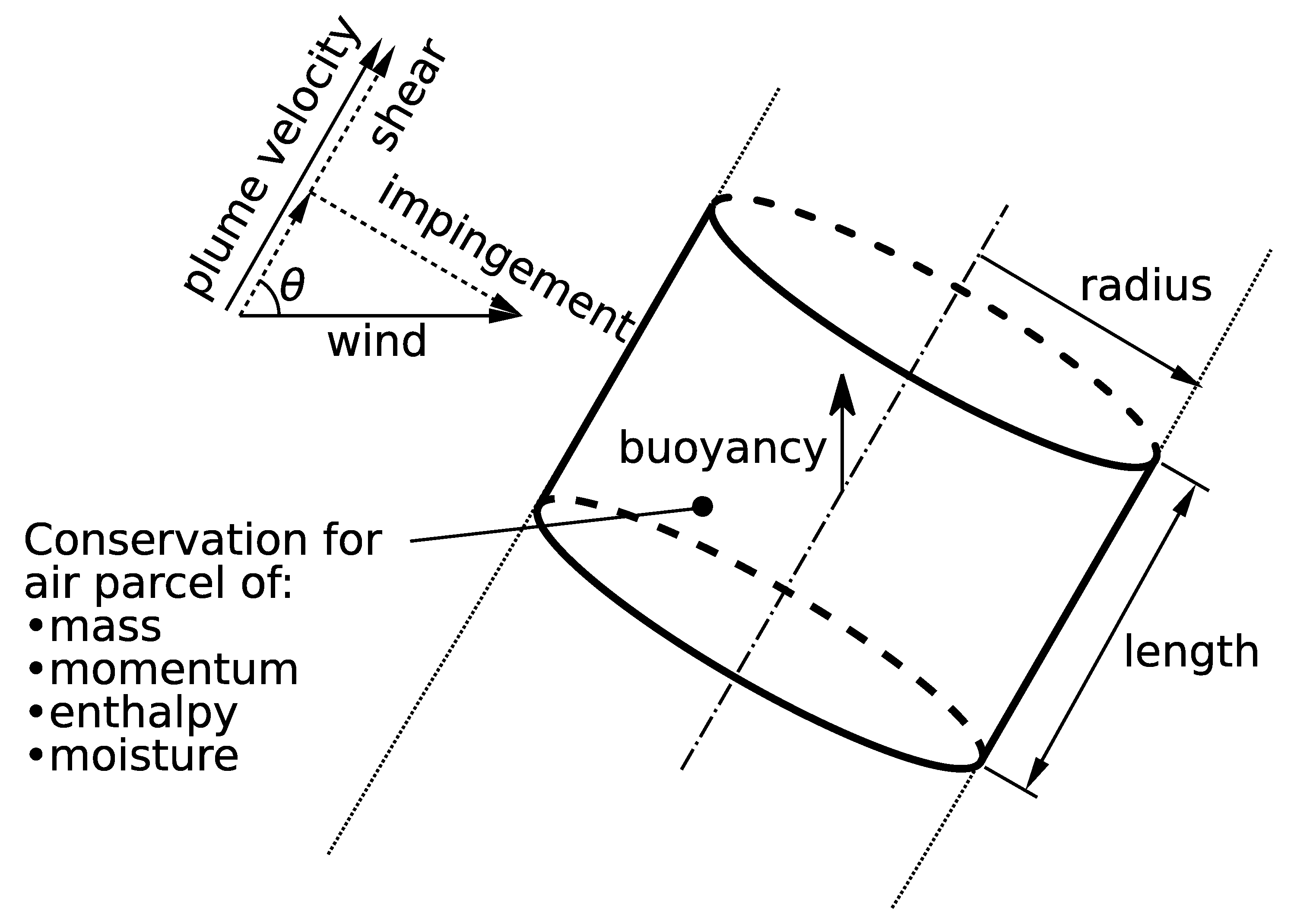
A one-dimensional model that integrates the conservation equations for mass, momentum, and energy along the plume axis (Figure 2) simulated a twelve-cell cooling tower where the cells are identical (Figure 1a). The cooling tower studied in this research is a GEA model 545436-12I-33-FCF that discharges 400 to 700 MW waste heat from a natural gas-fueled power plant in the southeastern United States that generates 500 to 900 MW of electricity. The cooling water line that connects the power plant to the cooling tower has a constant flow rate of 13.9 m³/s and is 6 to 11 °C warmer than the cooling water exiting the MDCT. Furthermore, the Hudson Tuf-Lite APT-32K-12 fans all run at a single RPM and the fan blades are set at a uniform pitch of 9 degrees. The twelve plumes in Figure 1a did not merge before they evaporated, but plume mergers do occur in calm conditions with high ambient relative humidity. The one-dimensional model simulated a row of individual cooling cells, where the height above the fill was 5.0 m. Each of the twelve cooling tower cells had a radius of 5.0 m and an area-averaged exhaust velocity of 6.0 m/s. The cell edges were 6.5 m from each other. Coordinate positions for each cell were used to combine individual plume simulations into a three-dimensional volume.

The model initially assumes a top-hat profile within the plume at a given elevation. A constant wind speed and direction, a flat terrain, and no obstacles such as buildings, vehicles, or trees were also assumed. The rate at which the cooling tower transfers thermal energy to the atmosphere via the cooling tower is given by:

$$Q_{liq}={\rho }_w{c}_{pw}{F}_{cw}\left(T_{cwin}-T_{cwout}\right),$$

(1)

where $Q_{liq}$ is the rate at which heat is removed from the process cooling water and transferred to the air passing through the cooling tower, ${\rho }_w$ is the density of water, $c_{pw}$ is the specific heat capacity of water, $F_{cw}$ is the process cooling water flow rate, $T_{cwin}$ is the process cooling water temperature entering the cooling tower, and $T_{cwout}$ is the process cooling water temperature exiting the cooling tower. The variables $F_{cw}$, $T_{cwin}$, and $T_{cwout}$ cannot be measured remotely, so Equation (1) cannot be used to find $Q_{liq}$. The corresponding energy budget equation for the air passing through the cooling tower remotely estimates $Q_{air}$, which is equal to $Q_{liq}$, aside from small radiative and conductive losses that occur as the air and water pass through the tower.

The entraining plume model requires lower boundary conditions to start the simulation. The required information is the enthalpy flux (sensible plus latent heat transfer rate to the atmosphere), MDCT exhaust volumetric airflow, and radius. The exhaust air is assumed to be saturated at the exhaust temperature. The following equation gives the starting conditions for the plume model:

$$Q_{air}={\rho }_a{C}_{pa}w\pi R_{ct}^2\left(T_{pl}-T_{air}\right)+{\rho }_{a}Lw\pi R_{ct}^2\left(q_{pl}-q_{air}\right),$$

(2)

where $Q_{air}$ is the enthalpy transfer rate (power), ${\rho }_a$ is the density of air, $C_{pa}$ is the specific heat of air, $w$ is the updraft velocity, $R_{ct}$ is the exhaust radius, L is the latent heat of vaporization, $T_{air}$ is the ambient air temperature, $T_{pl}$ is the exhaust air temperature, $q_{pl}$ is the specific humidity of exhaust, and $q_{air}$ is the specific humidity of ambient air. Equation (2) used increasing values of the exhaust air temperature until the enthalpy transfer rate was large enough to produce a simulated plume equal in size to the measured plume size.

The standard set of the one-dimensional entraining plume model equations was also taken from Carazzo et al. Conservation equations for water vapor and liquid water were added to the Carazzo et al. equations [1]:

$$\frac{dV}{dz}=2{\alpha }_e,$$

(3)

$$\frac{dM}{dz}=\frac{BV}{M},$$

(4)

$$\frac{dB}{dz}=-V{\mathsf{\Gamma }}_{air}\frac{g}{T_{air}},$$

(5)

$$\frac{d{T}_{pl}V}{dz}=\frac{dV}{dz}{T}_{air},$$

(6)

$$\frac{d{q}_{pl}V}{dz}=\frac{dV}{dz}{q}_{air+Evap-Cond},$$

(7)

$$\frac{d{q}_{liq}V}{dz}=Cond-Evap,$$

(8)

$$\frac{d{v}_{pl}V}{dz}=\frac{v_{air}dV}{dz}.$$

(9)

In the equation set above,

$$V=w{R}^2,$$

(10)

$$M=w^2{R}^2,$$

(11)

$$B=g^{\prime }w{R}^2,$$

(12)

where R is the radius of the plume, ${\mathsf{\Gamma }}_{air}$ is the ambient air potential temperature lapse rate, $v_{air}$ is the horizontal ambient wind speed, $v_{pl}$ is the horizontal component of the plume air velocity, q is the specific humidity, and the subscripts pl, air, and liq are for the exhaust, ambient, and liquid phases (visible droplets), respectively. Potential temperature accounts for differences in static air pressure density with height. It is incorporated into ${\mathsf{\Gamma }}_{air}$ by adding the dry adiabatic lapse rate (9.73 °C/km) to the actual lapse rate. The equation set was then solved from the bottom, starting with the boundary conditions at the top of the tower. The vertical discretization was 0.1 m. A predictor–corrector method solved the finite-difference equations, and the iterations were updated until the convergence criterion was obtained (plume temperature changes less than 0.001 °C in an iteration). A separate convergence criterion was applied to updraft momentum: the change in momentum in the most recent iteration relative to the previous iteration was required to be less than 0.01% of the previous momentum. The plume simulations are repeated with increasing initial exhaust air temperatures until the enthalpy discharge rate is sufficient to produce a simulated condensed water vapor (visible) plume with a volume equal to the measured volume. The air coming out of the cooling tower is assumed to be saturated.

The entrainment function, α_e, models entrainment of the ambient air for conditions where there was wind from the data set [25]:

$${\alpha }_e=R\left(\varphi \left|\sqrt{{v_{pl}^2+w}^2}-v_{air}cos\left(\theta \right)\right|+\beta \left|v_{air}sin\left(\theta \right)\right|\right).$$

(13)

In Equation (13), ϕ and β are entrainment coefficients with values of 0.085 [1] and 0.71 [25], respectively. The variable θ is the elevation angle of the plume axis relative to a horizontal surface. The first term in Equation (13) models the entrainment caused by velocity shear in the direction of the plume axis. The second term models the entrainment caused by velocity differences in the direction transverse to the plume axis.

The saturated plume exiting the top of the cooling tower will initially condense water vapor into small droplets with very small fall velocities, which are carried upward in the plume. As discussed above, some liquid water will be in the cooling tower updraft before it reaches the top of the stack. Unless the atmosphere is saturated, these droplets eventually evaporate. Condensation adds sensible heat to the plume and evaporation removes it. A realistic simulation of the plume includes droplet condensation/evaporation because a plume with condensed water vapor has higher temperature and greater buoyancy than the same plume without condensation. The evaporation/condensation in the plume is therefore calculated through an iteration loop until the water mass and thermal energy are conserved.

Visible plumes composed of water droplets initially increase in width as they rise but then contract before evaporating entirely. This implies that liquid water density is significantly greater in the core of the plume than in the periphery. Laboratory measurements by Kotsovinos demonstrated that the radial profiles of temperature, velocity and other plume parameters fit a normal probability (Gaussian) function [16]. This means that the inner core of an entraining turbulent plume created by MDCT exhaust will have higher temperatures, specific humidity (gas and liquid), and velocities than the edges.

The clear implication of the radial Gaussian profiles in turbulent jets is that the turbulent mixing of properties from the core of the plume to the adjacent environmental air is accomplished by randomly distributed turbulent eddies. The random fluctuations in plume properties will average out, resulting in the well-known Gaussian plume. It is expected that individual model predictions differ significantly from any individual plume, but the average model prediction for many plumes should be close to the average measured values.

The model described above produces single average values of plume properties at a given elevation. Since the actual plume variables will decrease with the distance from the center, it is expected that the predicted model average will be lower than the core values, including liquid water content, which means that the model should, on the average, under-predict the maximum visible plume elevation. Application of the Gaussian profile should correct this. The plume radial temperature and water concentration profiles are then defined by:

$$q_{plm}=\left(q_{max}-q_{amb}\right)\mathit{exp}\left(-\frac{r^2}{2{\sigma }^2}\right)+q_{amb},$$

(14)

$$T_{plm}=\left(T_{max}-T_{amb}\right)\mathit{exp}\left(-\frac{r^2}{2{\sigma }^2}\right)+T_{amb}.$$

(15)

Define:

$$∆q=q_{max}-q_{amb},$$

(16)

and

$$\overline{q_{plm}}=\frac{{\int }_0^{R_{plm}}{q}_{plm}\left(r\right)dr}{R_{plm}}=\frac{∆q}{R_{plm}}{\int }_0^{R_{plm}}exp\left(-\frac{r^2}{2{\sigma }^2}\right)dr+q_{amb},$$

(17)

where $R_{plm}=2\sigma$ and is converted to the standard error function erf $\left(r\right)=\frac{2}{\sqrt{\pi }}{\int }_0^{r}exp\left(-\frac{t^2}{2}\right)dt$, $t=\frac{r}{\sqrt{\raisebox{1ex}{$1$}\!\left/ \!\raisebox{-1ex}{$2$}\right.}{R}_{plm}}$ where $r=R_{plm}$, and where $q_{max}=1.67\left(\overline{q_{plm}}-q_{amb}\right)+q_{amb}$ with corresponding equation for $T_{amb}$. As a condition, a plume is considered visible until $q_{max}<q_{sat}$.

It is noted that some MDCTs, including the site of our empirical measurements, have ten or more cells in a row. Individual cell plumes in a row with many cells will not develop as they would if they were far from the other plumes in the row because as the plumes rise and spread, they will mix and interact. Relative to a single isolated cell, multiple plumes shield each other, to some degree, from entrainment of drier environmental air. The shielding will cause the maximum heights of plumes in a row, on the average, to be somewhere between the height that an equivalent area single-cell plume would reach and the height that an individual cell in the row would reach if it was isolated from the rest of the cells and their plumes.

The following approach was developed to extend the one-dimensional code to account for plume interactions: run the one-dimensional model as a single cell with an area equal to the combined areas of all cells and account for the increased entrainment experienced by the row of smaller plumes relative to a single large plume. Generally, the semi-empirical, heuristic extension of the one-dimensional model should depend only on the basic geometric features of an MDCT, such as cell number, diameter, and spacing. All 12 cells of the MDCT have radii of 5.0 m ($r_0$), and the combined area of these 12 cells is equal to a single cell with a radius, $r_{00}$, of 17.3 m:

$$r_{00}=\sqrt{{N_{c}r}_0{r}_0},$$

(18)

where N_c is the numbers of cells (12). In this approach, the simulation starts with the plume radius $r=r_{00}$. The twelve cells have a greater combined perimeter than the equivalent single cell: $p_1=N_{c}2\pi r_0$ is larger than $p_2=N_{c}2\pi r_{00}$. Since the twelve plumes have a larger initial “boundary” with the surrounding atmosphere, the entrainment of ambient air into the 12 cells will be greater than the entrainment into the equivalent single cell. However, since the cells are arranged in a row, the additional entrainment will be a function of the wind direction relative to the orientation of the axis of the cell row. There exists shielding of downwind cells when the wind direction is parallel to the cell axis, and less when it is normal to the cell axis. To account for this effect, several parameters are defined. The first is a radius equal to the radius of a plume with the combined areas of the N_c plumes:

$$r_{eq}=\sqrt{N_c{r}_{sh}{r}_{sh}},$$

(19)

where $r_{sh}$ is the radius of an individual cell plume.

The next parameter is ${\theta }_d$, which is the difference between the wind direction and the azimuth of the row of MDCT cells relative to north. A parameter, $b_1$, is next defined as:

$$b_1=\left(\pi r_{sh}+d_l\left|sin\left({\theta }_d\right)\right|\right)/\left(\pi r_{sh}+d_l\right),$$

(20)

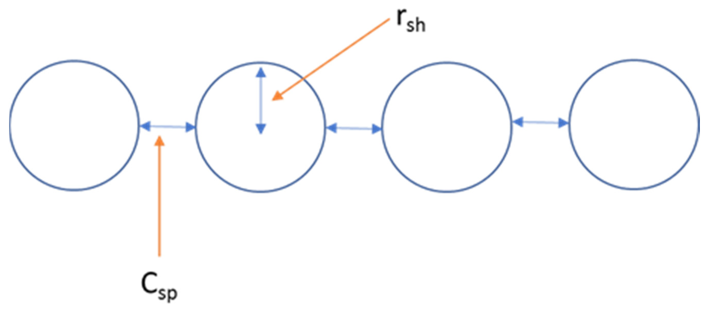
where $d_l$ is a length scale for the row of cells:

$$d_l=\pi \left(N_c-1\right)r_{sh}+\left(N_c-1\right)C_{sp}.$$

(21)

In this equation, $C_{sp}$ is the gap between the edges of adjacent cell shrouds as shown in Figure 3. The parameter $b_1$ is designed to maximize entrainment when the wind is blowing perpendicular to the row of MDCT cells and minimizes it when the wind is blowing parallel to the row of MDCT cells. The next parameter, $a_1$, is designed to account for the additional entrainment that a row of plumes will experience relative to a single cell that started with the equivalent area to the N_c cells combined:

$$a_1=\frac{\left(2\pi N_c{r}_{sh}\right)}{2\pi r_{eq}}=\sqrt{N_c}.$$

(22)

Equation (13) is therefore modified by incorporating $a_1$ and $b_1$:

$${\alpha }_{em}=R\left(a_1\varphi \left|\sqrt{{v_{pl}^2+w}^2}-v_{air}cos\left(\theta \right)\right|+b_1\beta \left|v_{air}sin\left(\theta \right)\right|\right).$$

(23)

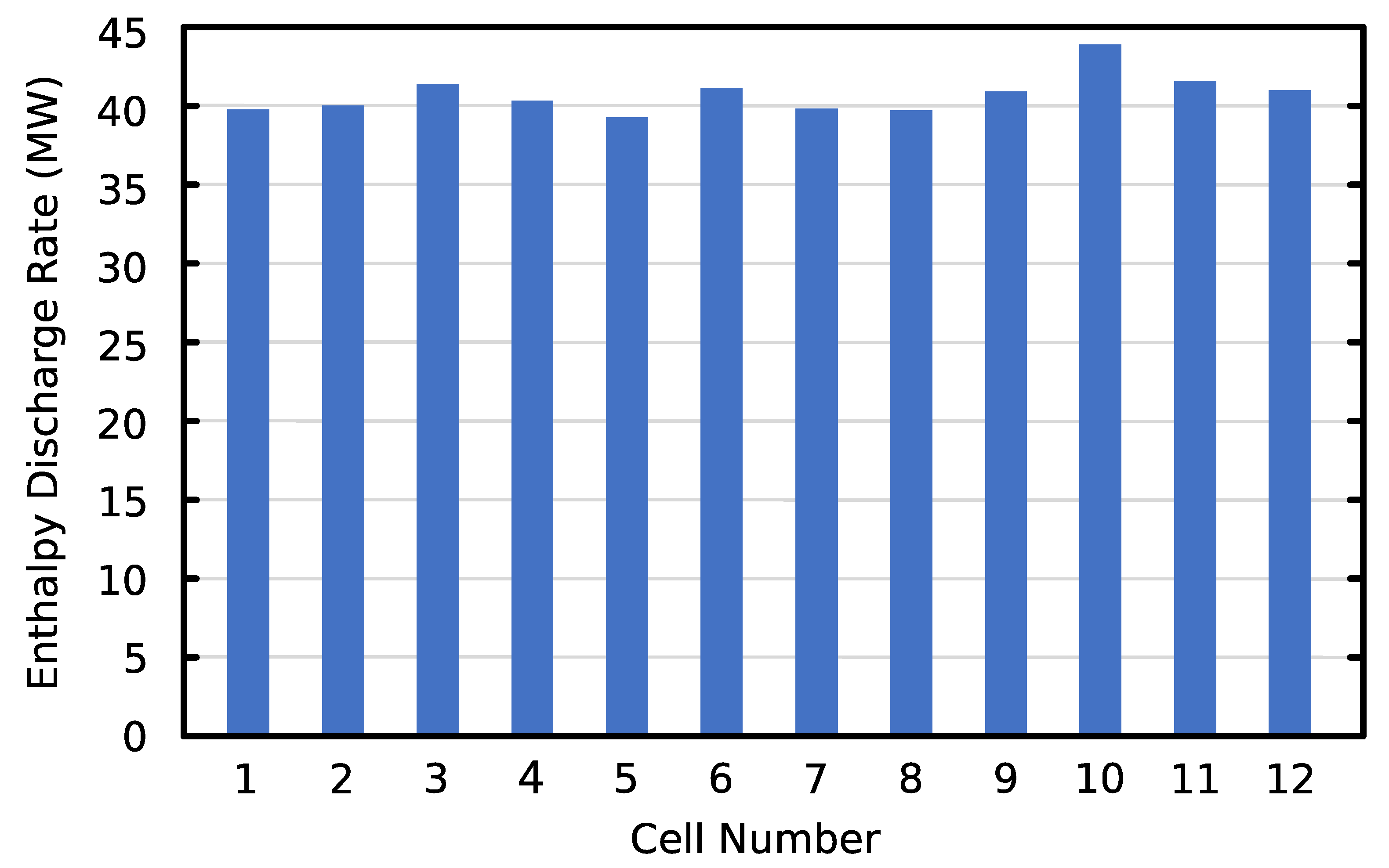
We note that inside water-cooling towers, there can exist maldistribution of water flows as demonstrated by previous authors [26,27], but at the twelve-cell water cooling tower site in the southeastern U.S., the enthalpy transfer rates for all twelve cells are nearly identical with variations of 2 to 3% except for the tenth cell, which was 8% higher than the average as seen in Figure 4. This indicates that on a cell-by-cell basis, the thermal energy transferred from the cooling water to the air flowing through the cooling tower is the same to within a few percent. Although the figure shows slightly unequal distribution of the flow in the tower, it is small and assumed uniform for the purpose of this study. The MDCT analyzed in this paper operates at a humid subtropical site in the southeastern U.S., which has very low average wind speeds (~1 m/s). This model can also be used for winter and summer applications, but it does not account for the impact of freezing conditions on plume thermodynamics and does not simulate precipitation, which can be produced by very large plumes in cold weather.

3. Plume Volume Measurements

Plume volumes were measured using imagery from 8 stationary camera stations deployed around the cooling tower as illustrated in Figure 5. Because off-the-shelf three-dimensional reconstruction tools, based on Structure from Motion, are poorly suited to the plume’s indistinct features and changing shape over time, a novel analysis was developed to determine plume volumes. This technique, detailed by our collaborators in Connal et al., uses a neural network-based image segmentation algorithm to identify the plume in each image and a space carving technique to estimate the volume of the plume [19]. Cameras were each calibrated, and camera pose (location and orientation of the installed camera) was determined using Structure from Motion on the solid structures in the scene. A model, based on Matterport Mask R-CNN, was trained to identify the plume in each image, using manually annotated data [28]. As visualized in Figure 6 and in Connal et al.’s study, the image segmentation model determines both a boundary box for the plume and classifies the pixels as plume or not-plume within the boundary box [19]. Different results of Mask R-CNN performances were also displayed in Connal et al.’s study [19]. Finally, the plume volume was estimated by dividing the domain into voxels and “carving” away any portion of the domain on a line of sight identified as not-plume from the image segmentation in any of the 8 camera angles, also seen in Figure 5. The project has also collected imagery for plume volume measurement via unmanned aerial vehicle flights, but ground station data have been used for plume model development due to the greater number of samples and wide variety of weather conditions seen during the continuous field study. A total of 289 data points—each based on analysis of images from all of the 8 ground station cameras—were used in this study. The data yielded plume volumes from 1274 to 2,247,000 m³.

The 8 camera stations deployed around the site each contained identical hardware consisting of a Canon M200 mirrorless camera, solar charging, a Raspberry Pi-based GPS timing and communications module, and weatherproof case. The stations were distributed around the perimeter of the cooling tower site to capture all sides of the plume and distances as far as practical within the open space around the cooling tower. Prior to deployment, the field of view from each camera was modeled in Blender [29], resulting in the selection of a Canon 10–18 mm ultra-wide-angle lens to obtain an acceptable height of plume capture.

4. Weather Data and Model Inputs

The one-dimensional model used averaged weather data from 11 regional airports. Some of these stations are in urban areas (Charleston and Columbia, SC, USA; Savannah, GA, USA; and Jacksonville, FL, USA), some are associated with military bases (Beaufort, SC and Hunter Field, GA, USA) and others are smaller, more rural airfields (Walterboro, Orangeburg, Barnwell, and Hilton Head, SC; and Waycross, GA, USA). The National Oceanic and Atmospheric Administration (NOAA) has primary responsibility for weather data collection, but management of smaller airfields is often the responsibility of the Federal Aviation Administration (FAA). An onsite weather station’s data were not used because the measurements were made near a floodplain forest which affected both relative humidity and wind speed. Airport weather stations are in open areas with no nearby buildings or trees and thus are more representative of conditions at the discharge level of an MDCT, which is typically 10 to 15 m.

Simulations of the measured plume volumes require input files for the weather and MDCT layout (number of cells, cell diameter, cell spacing) as well as entrainment coefficient data (Equation (23)). The main input file contains ten variables such as date/time, ambient air temperature, dewpoint temperature, wind direction (degrees from north), wind speed (m/s), air pressure, measured plume volume, number of cells with fans on, cell-area average exhaust velocity at 6.3 m/s, and vertical temperature gradient at −6.5 °C/km (the NOAA standard atmospheric lapse rate). The model validation data are average cell exhaust air temperature and measured power. Another input file includes entrainment coefficients and cooling tower geometric parameters such as number and spacing of cells.

5. Model Simulations Results and Discussion

For each of the 289 measured plume volumes, multiple one-dimensional model runs were performed using ascending exhaust air temperatures until the simulated combined plume volume exceeded the measured value. Each of the simulated plume volumes had a corresponding enthalpy discharge rate (power) to the atmosphere (exhaust air was assumed to be saturated). The simulated plume volume greater than the measured volume and the volume from the preceding iteration were used to linearly interpolate the corresponding powers to the value expected for the measured volume.

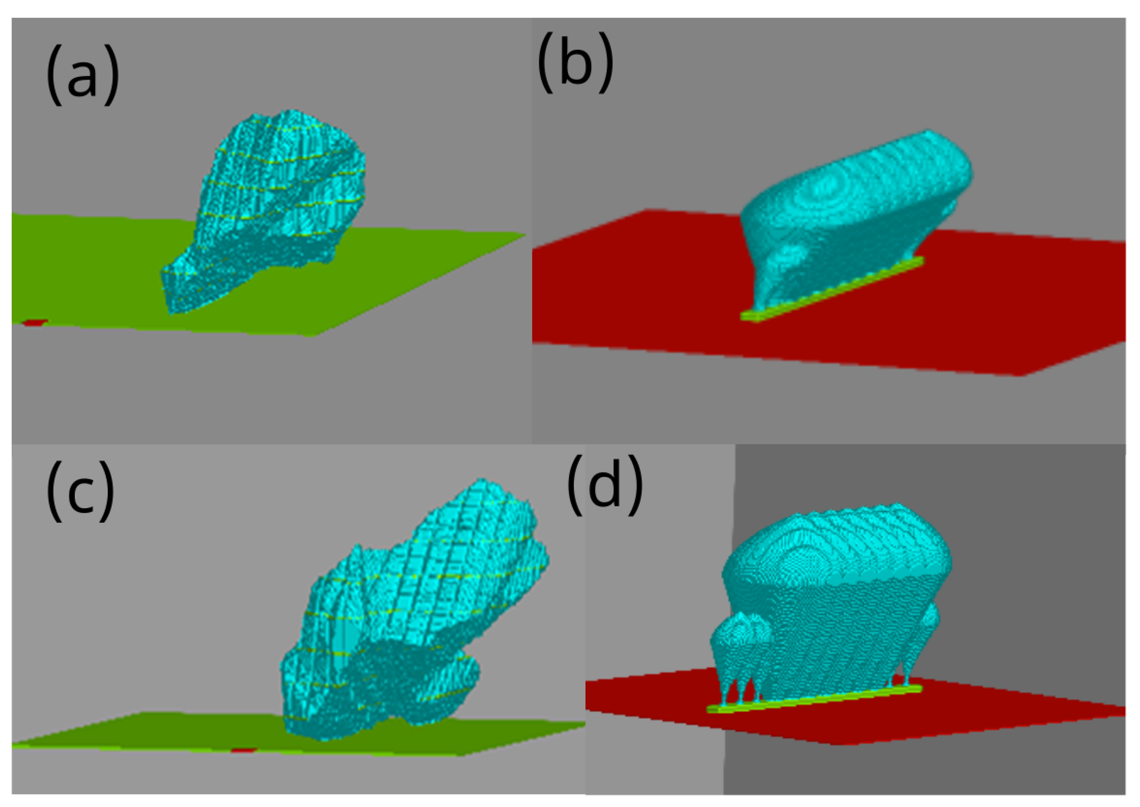
Figure 7 compares plumes created by combining multiple simultaneous digital photos to corresponding plumes created by combining multiple simulations of one-dimensional plumes into a single volume representing twelve cells. The measured plumes are highly irregular and appear to capture the denser parts of the plume but not the fringes, when compared to Figure 1. Eight cell fans were on when the digital imagery was taken and created the plume shown in Figure 7a,b. Figure 7c,d show images for a time when seven fans were on and five were off. The cells with fans off are obvious in Figure 7b,d because buoyant convection produces a much smaller plume relative to forced convection. There is some evidence of smaller buoyant plumes at the ends of the measured volume in Figure 7a,c, but they are much less obvious. The shapes of the simulated and measured plumes can only roughly agree because the simulations are from a one-dimensional code, and because the measured plume is irregular due to turbulent eddies in the wind that constantly deform the plume from the idealized simulated plume that was created using regionally averaged weather data.

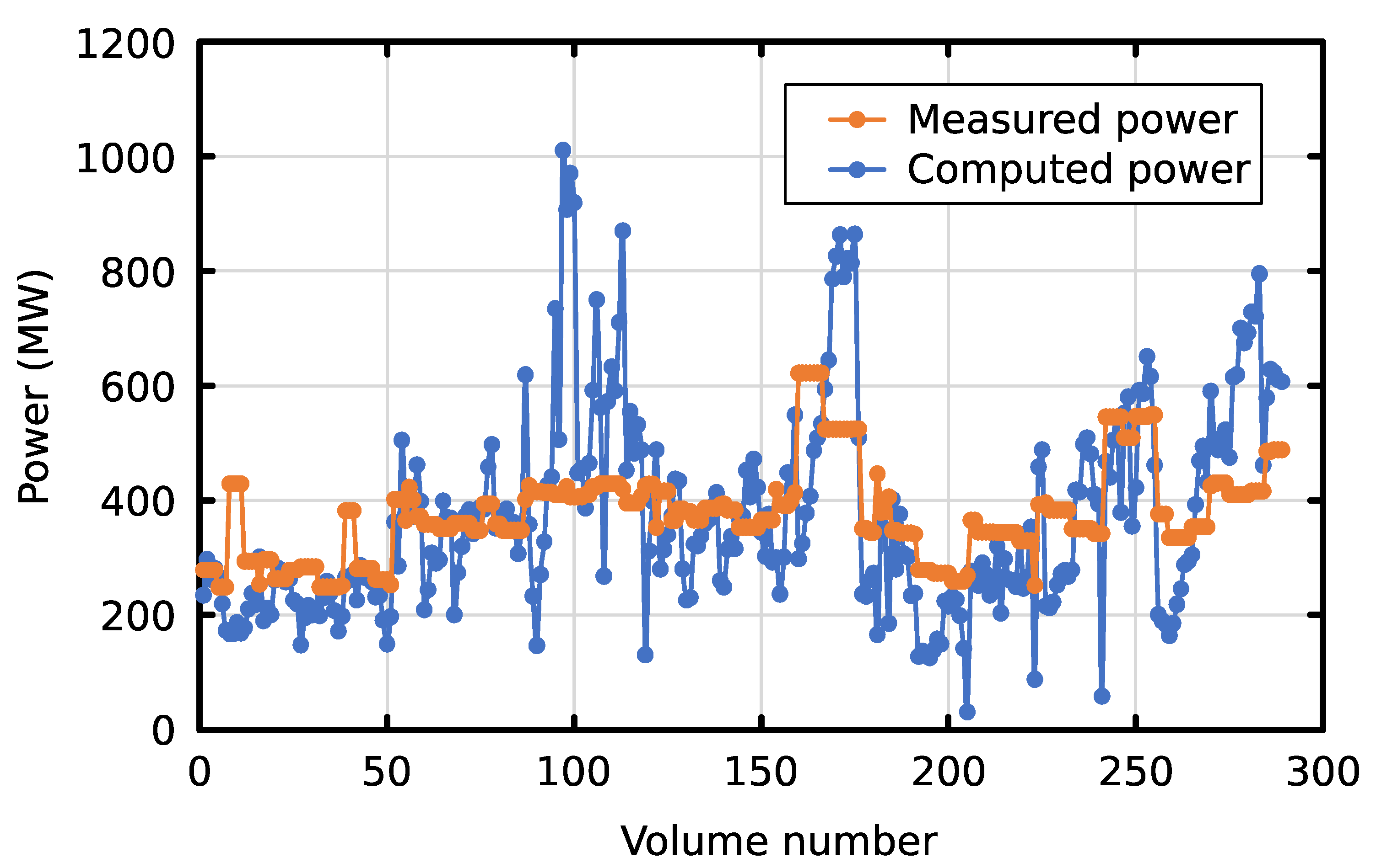
The model was primarily validated based on the averaged computed and measured powers. Figure 8 shows that on an individual plume volume basis, the one-dimensional model could greatly over or underestimate observed power output. However, when the average meteorological data for all 11 stations were used as model input, the averaged power from the calculated and measured powers were 343 MW and 378 MW, respectively, giving an error of about −10%. The correlation coefficient for measured and computed pairs was 0.60 and the average absolute error was 103 MW. The large error for individual pairs of measured and computed powers is mostly attributable to the uncertainty in the meteorological data, specifically the dewpoint temperature depression (DPTD).

The one-dimensional model assumes a Gaussian distribution of properties (updraft velocity, temperature, liquid water content) around the centerline of the plume. It is well known that time-averaged turbulent plumes have Gaussian distributions of properties. So, it is appropriate to expect that the average of many measured plume volumes will be close to the average simulated volume, even though on an individual basis the simulated volume may be very different from the measured volume. This implies that the average computed power will also be closer to the average measured power than individual pairs of measured and computed powers. The larger standard deviation of the simulated powers in Figure 8 relative to the measured power standard deviation is the consequence of using a one-dimensional model that can only simulate Gaussian (average) plume shapes and volumes. Sometimes, the simulated powers will be greater than the measured powers and sometimes they will be smaller, as can be seen in Figure 8. If the regional meteorology is representative of the average weather conditions at the cooling tower, and the enthalpy flux from the cooling tower is correct, the average measured powers should be about equal to the average simulated powers because the average measured plume will be Gaussian, like the model plume.

Figure 9 shows how the one-dimensional model’s ability to predict average power varied according to which of the 11 regional airport meteorological data sets were used as code input. Results are also shown from simulations that used average weather data from all 11 stations and from the six more urban or military sites (Charleston, Columbia and Beaufort, SC, USA; Savannah and Hunter Field, GA, USA; and Jacksonville, FL, USA). The meteorological variable that is plotted is the DPTD at the time the digital imagery of the cooling tower plumes was collected. The DPTD was chosen because it has the greatest meteorological impact on plume volume (correlation coefficient of 0.79). The average ratio of computed-to-measured power for the six urban or military sites is 0.98 and the average ratio for all eleven sites is 0.91. The five more rural sites produced an average ratio of 0.79. The reason for the difference in model performance as a function of which stations were used in the averages is not known. It could be an effect of urban heat islands which would increase air temperature and lower dewpoint temperature, both of which increase DPTD and cause the model to require more power to produce the same volumes. Alternatively, the smaller, more rural airports may be more influenced by nearby forests which would lower air temperatures and raise dewpoint temperatures relative to the more urban airports.

The computed power ratios are less than 1.0 for all three average meteorological datasets (all 11 stations, 6 NOAA/DOD stations, 5 rural stations). This bias may be attributable to model deficiencies or the average plume volume measurements may be low. When Figure 1 is compared to Figure 7, it would appear feasible that the wispy edges of the visible plumes are not captured by the space carving technique. More plume volume measurements will be available in the future, which may make it possible to determine if, for the same meteorological conditions and power, plume images with sharp edges produce larger volumes than plume images with wispy, less distinct edges. This topic is discussed further in the next section.

6. Uncertainty Analysis

Several variables contribute to the uncertainty of the one-dimensional model predictions of enthalpy transfer rate (power) from the cooling tower to the atmosphere: measured plume volume, meteorological data, entrainment coefficients, and other limitations of a one-dimensional model. The DPTD is highly correlated with the computed power as shown in Figure 9 (R² = 0.79), and this meteorological variable is the largest source of uncertainty in the weather data inputs. Correlation of the 11 individual station power ratios with dewpoint temperature depression in Figure 9 shows that a 1 °C error in average DPTD produces a 17% error in the average computed power. The averaged meteorology produced smaller errors than 17%, so it appears that the averaging produced an average DPTD error of less than 1 °C.

Data presented by Carazzo et al. shows a range from about 0.06 (buoyant convection) to about 0.13 (forced convection) for the entrainment coefficient ϕ in Equations (13) and (23) [1]. The one-dimensional model simulations described in this paper used a value of 0.085, which is intermediate between buoyant and forced convection but closer to the buoyant convection values. The value of 0.085 was chosen because the plumes are observed to transition rapidly from forced to free convection. A survey of experimental results for the other entrainment parameter (β) in Equations (13) and (23) found a wide range of values from 0.3 to 2.0 [25,30,31,32,33,34]. A sensitivity run was conducted with the one-dimensional code using a value of ϕ of 0.12 and a value of β of 1.0. Since these values are higher than the baseline values of 0.085 and 0.71, they increased entrainment of ambient air which required higher powers to produce the observed plume volumes. The ratio of computed to observed power rose from 0.91 to 0.97 when the 11-station average station meteorology was used.

When Equation (13) was used to simulate the 289 volumes instead of Equation (23), the computed-to-measured power ratio dropped from 0.97 to 0.91 (using average meteorology from the six NOAA or DOD stations). When meteorology averaged from all 11 stations was used, the power ratio dropped from 0.91 to 0.84. The power ratio dropped in both cases because entrainment of ambient air was reduced. This suggests that the alterations in Equation (23) to model adjacency effects of multiple plumes in a row moderately improved model performance by more correctly computing entrainment.

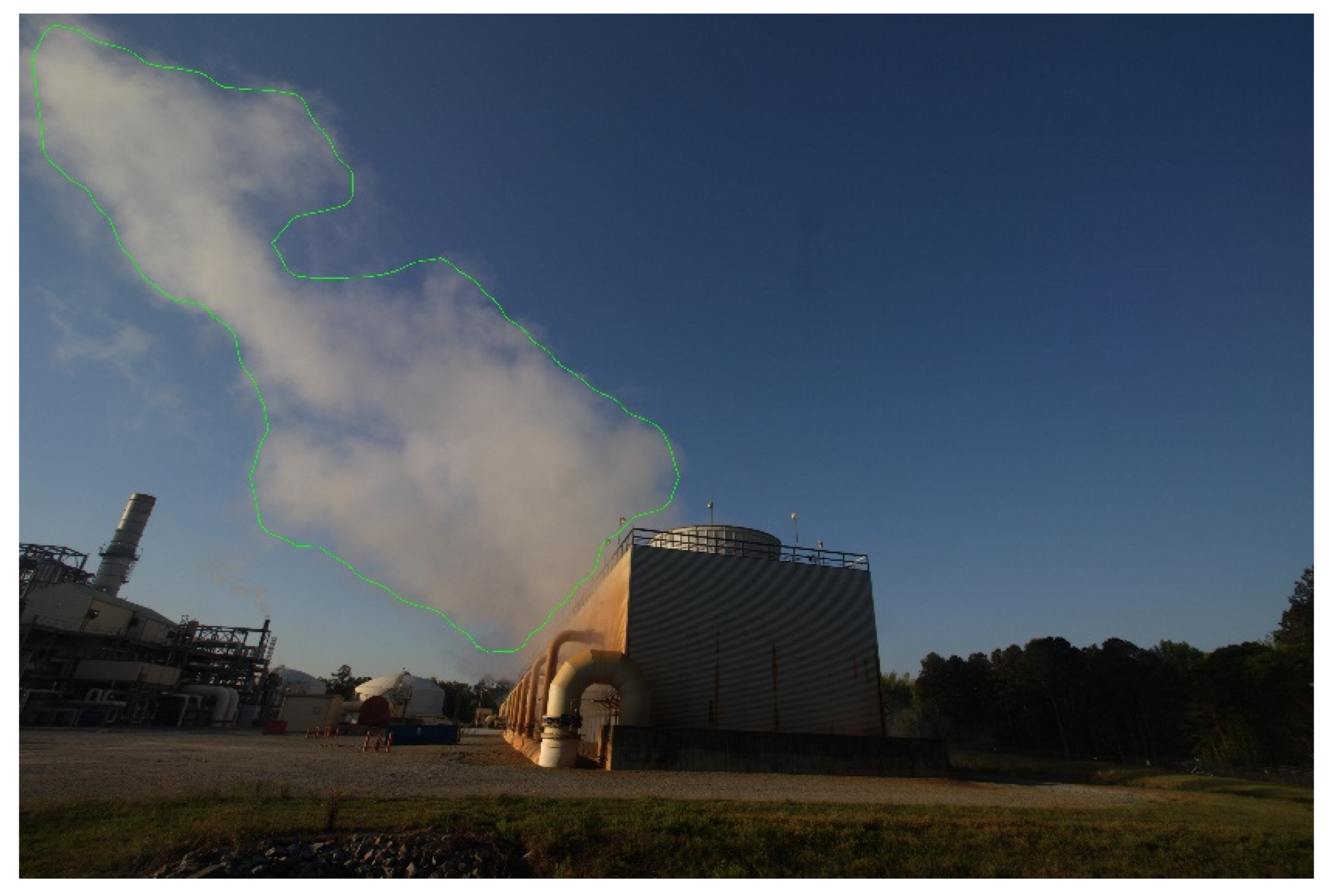
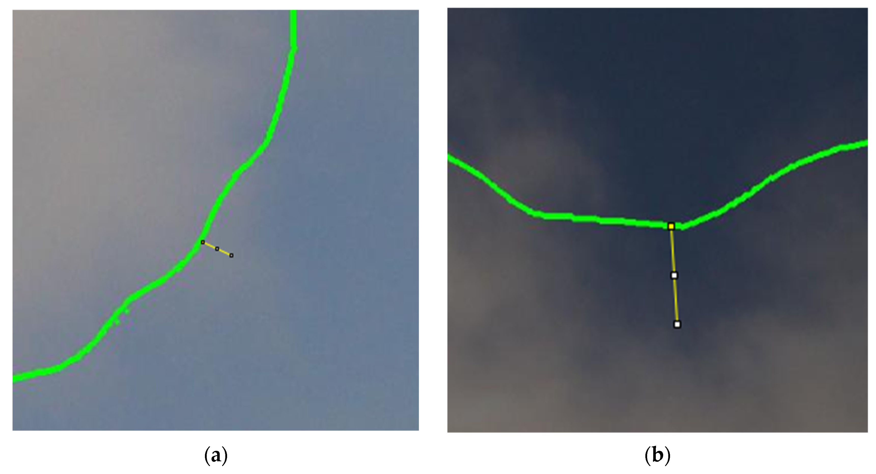
Figure 10 is an example of a ground-based digital image of a cooling tower plume with the mask for that plume outlined in green. Small areas of the plume that are separate from the main body of the plume are not within the mask boundary. Within the mask boundary some parts of the plume are more optically thick than others.

The uncertainty estimation of the plume volume measurements lies within the plume mask generation for boundary decision and space carving voxel density with uniform volumes for reconstruction. While considering the initial boundary of three-dimensional voxels, the individual volume of all voxels within this space can affect the resulting volume. Plume volume estimates were based on space carving voxel densities where a uniform size of voxels ranged between 0.1 and 1.0 m³. For plume mask generation, the model inferences produced by Mask R-CNN provide estimates of the plume boundary. For the uncertainty procedure, 60 plume images with the model inference mask were analyzed, in which 30 locations were sampled along the border of each mask. At each location, the distance in pixels from the edge of the model inference mask to the visible plume boundary was measured. A positive distance indicated the plume boundary was outside of the mask at that sample location, a negative distance for when the boundary fell within the mask, and zero when the two were aligned. Based on 1800 pixel distance measurements, the average distance from the model inference segmentation mask to the observed plume boundary was 11.2 pixels. A negative measurement would indicate that on average the model is overcompensating, but the result was positive, which reveals that the average inference mask needed to be expanded by approximately 11 pixels uniformly along the edge of the entire boundary. Figure 11 shows examples of mask boundary adjustments that were made to more correctly track the true plume boundary.

The volume uncertainty procedure uses the morphology operation of dilation to uniformly expand the model inference masks by 11 pixels and compare against the plume volumes produced by the model. This analysis was conducted on 50 cases, where the volumes produced by the dilated masks were treated as the ground truth. The volumes were calculated and averaged from the voxel densities ranging between 0.1 and 1.0 m³ for all cases. To uniformly expand the masks by 11 pixels, a 23-pixel by 23-pixel kernel was used to implement a dilation operation, which adds pixels to the boundary of the mask. By operating on pixels centered at the origin of the kernel, the mask is expanded uniformly in all directions within a distance of 11 pixels.

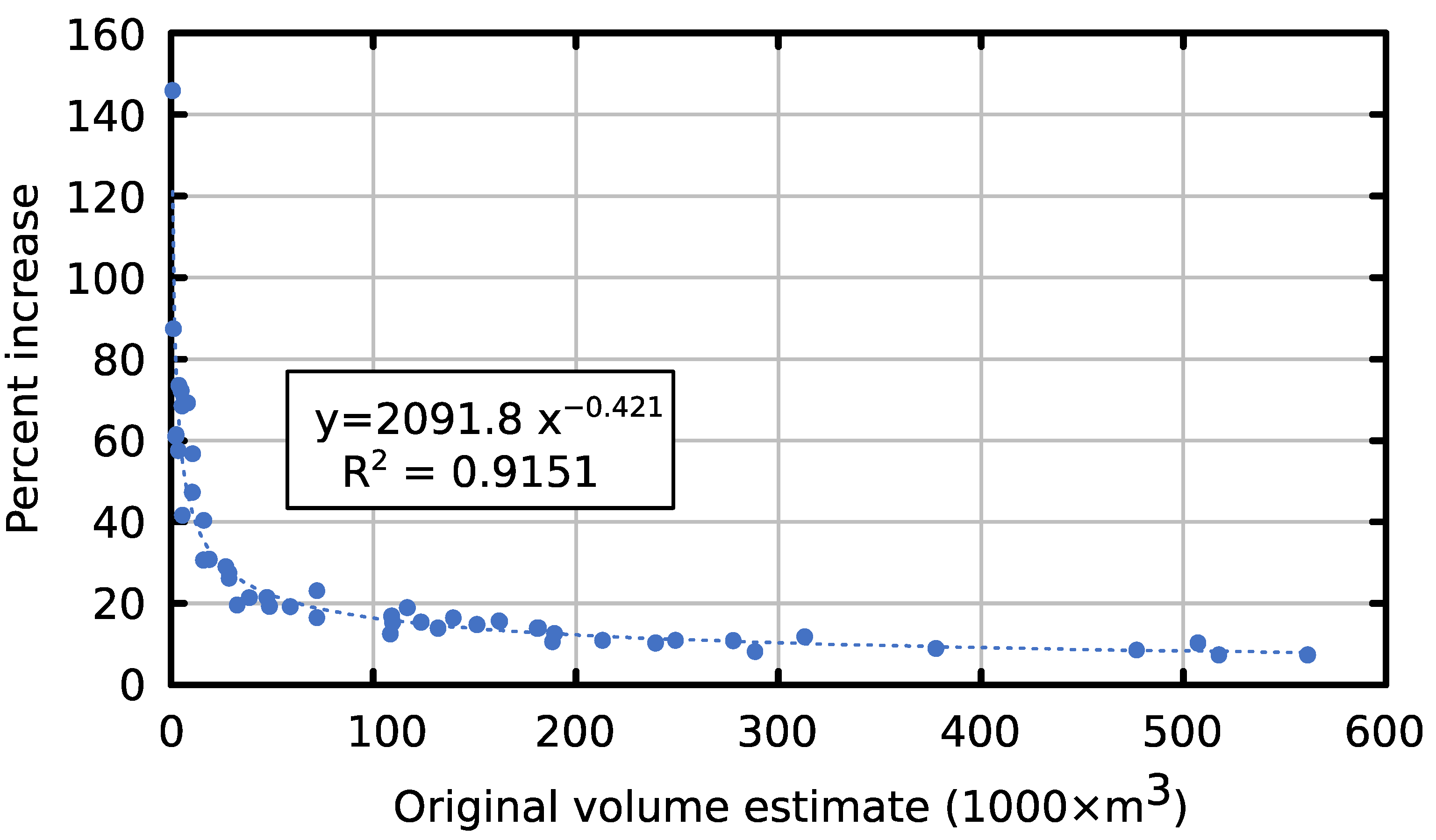
The differences between the original 50 plume volumes produced by Mask R-CNN and the dilated volumes are shown in Figure 12. The differences are expressed as percent increase in volume relative to the original volumes. The large percent increases are associated with the smallest volumes. This is attributed to the rapidly decreasing percentage of an 11-pixel surface layer on a volume relative to the total plume volume as it increases. The power law fit to the data in Figure 12 represents the uncertainty in the plume volume measurements expressed as percent increase in plume volume from the original undilated measurements.

The power law fit to the data in Figure 12 was used to increase the original 289 volume estimates. The one-dimensional plume model was run with the 289 modified volumes, which produced the average power estimates for different meteorological data sets as discussed and shown in the previous section of this paper. When the one-dimensional model was run with what is believed to be the best meteorological data (average of six NOAA and DOD stations) the average power computed from the undilated volumes was 94% of the measured average. The average power computed from the dilated volumes was 98% of the measured average. Based on this uncertainty analysis, it appears that the plume volume measurement uncertainty is a small contributor to the uncertainty of the average power estimate derived from the plume volume measurements and other model input variables.

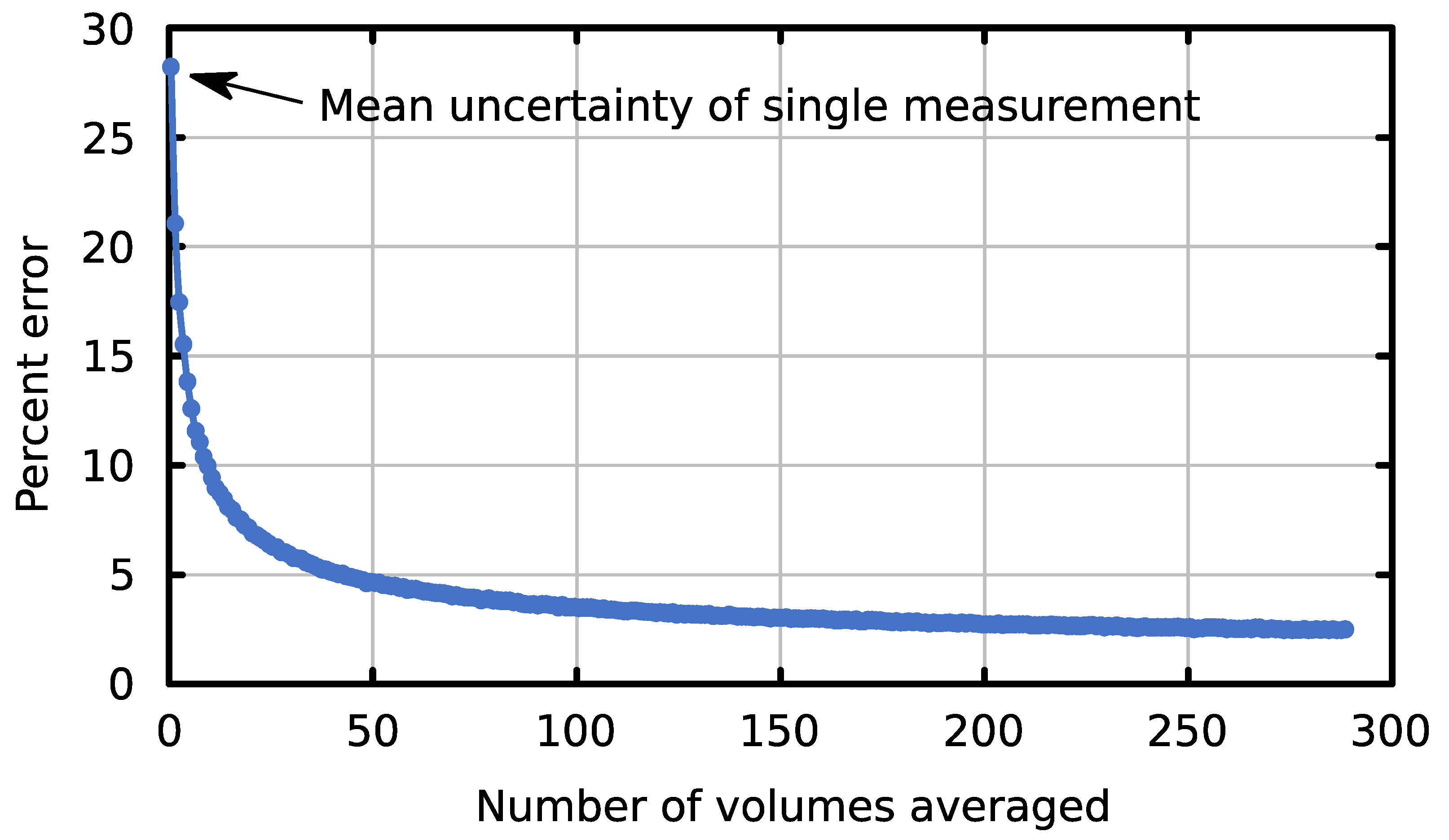
The average rate of power generation is a more reliable indicator of fuel consumption than an estimate based on a single plume volume. The effect of random errors in the meteorological data and plume volume measurements largely average out when many plume volumes are used to compute the average power. This is clearly apparent in Figure 13, which shows the results of averaging the differences between pairs of measured and computed powers. Averages were computed by randomly selecting pairs from the 289 available. The procedure started by selecting single pairs 10,000 times and computing the average. Then two pairs were selected and averaged 10,000 times and the 10,000 averages were averaged. This process was repeated for three pairs, four pairs on up to 289 pairs. Figure 13 shows that 50 pairs produce an average error of 4.5% which is only slightly larger than the average error for all 289 pairs (2.4%).

The current uncertainty analysis of the plume volume, based on ground-based imagery and the method for volume quantification, is an initial investigation that may require additional comparisons for future research. For example, three-dimensional ray tracing combined with realistic water droplet distributions generated by three-dimensional simulations may produce more accurate plume boundaries with Mask R-CNN. The inclusion of a three-dimensional plume study could use a variety of mesh adaptations/distributions (i.e., a mesh-independent study) and additional physics-based models to accurately simulate the plume boundary.

7. Conclusions

A modified one-dimensional entraining plume model predicted average MDCT enthalpy discharge rate to the atmosphere (power) to within about 9% (343 MW computed versus 378 MW measured). These results were based on 289 measured plume volumes derived from multiple simultaneous digital images of the visible plumes. A one-dimensional plume model used average meteorology from 11 regional weather stations to predict cooling tower enthalpy dissipation rate (power). When average meteorology was computed from six urban or military sites the ratio improved to 0.98. The power ratio dropped to 0.79 when the average meteorology from five rural airfields was used. The correlation coefficient for individual pairs of measured and computed powers was 0.60. Since accurate average CO₂ emissions are needed for assessment of potential climate impacts, the one-dimensional model average power determinations are of primary interest. While the power output is essential to investigate emissions, issues regarding power consumption needs to be further investigated in a future project paper. The results presented here appear to justify further research: three-dimensional modeling to determine the importance of fundamentally three-dimensional phenomena such as plume mergers, and AI (artificial intelligence) applications to improve model performance and improved meteorological input.