
Simulation and Estimation of the Inter-Source Category and/or Inter-Pollutant Emission Offset Ratios for a Heavy Industry City

Department of Safety, Health and Environmental Engineering, National Yunlin University of Science and Technology, Yunlin 64002, Taiwan
*
Author to whom correspondence should be addressed.
Atmosphere 2023, 14(4), 748; https://doi.org/10.3390/atmos14040748
Submission received: 20 March 2023
/
Revised: 11 April 2023
/
Accepted: 18 April 2023
/
Published: 20 April 2023
(This article belongs to the Section Air Quality)
Abstract
:Kao-Ping Air Basin (KPAB) is a heavy industrial area, and also the first and only air quality total quantity control district in Taiwan. Pollutant emission offsetting is an important tool to reduce pollution source emissions and improve air quality in the total quantity control district. In this study, an air quality model was employed to evaluate the sensitivity of SOX, NOX, and primary PM2.5 emissions from point, mobile, and fugitive sources on PM2.5 concentrations in KPAB. The findings show that the emission offset ratios of mobile PM2.5-to-point PM2.5 and fugitive PM2.5-to-point PM2.5 were both greater than one in urban areas (1.3 and 2.0, respectively) and both less than one in non-urban areas. The offset ratios of point SOX-to-point PM2.5 and point NOX-to-point PM2.5 were significantly greater than one, especially those in urban areas (20 and 60, respectively) were higher than those in non-urban areas by more than 2–4 times. No matter whether in urban or non-urban areas, the offset ratio of mobile NOX-to-point NOX was close to one, and the offset ratios of point NOX-to-point PM2.5 and mobile NOX-to-point PM2.5 were similar. The above findings were closely related to the proximity of point sources to densely populated urban areas in KPAB.
1. Introduction
In Taiwan, autumn and winter are the seasons with the worst air quality, and fine suspended particles (PM2.5) are one of the main pollutants causing poor air quality. KPAB (Kao-Ping Air Basin) is a heavy industry area with intensive petrochemical, steel, and power industries. On top of that, its topography and climatic conditions make the PM2.5 and ozone concentrations higher than that observed in other parts of Taiwan [1]. To this day, KPAB is still an area that does not meet the PM2.5 air quality standard. Its average PM2.5 concentration in 2021 was 19.7 μg/m3, and its annual unhealthy (>35 μg/m3) station day occurrence percentage was as high as 10.1% [2]. To better improve the air quality in KPAB, Taiwan Environmental Protection Administration (TEPA) announced KPAB as a total quantity control district [1]. According to the Air Pollution Control Act revised in 2018 [3] and the Offset Principles for the Increased Air Pollutant Emissions Caused by Development Activities enacted in 2009 [4], revised in 2022 [5], and promulgated by TEPA, in total quantity control districts, new or existing stationary sources that increase emissions beyond a certain level must employ the best available control technologies but can obtain sufficient emissions from stationary, mobile, or fugitive sources in the same district to offset their increased emissions.
According to the original offset principles (enacted in 2009) in Taiwan, the offset ratios between pollutants are provided as follows: 200 tons of NOX (nitrogen oxides) emissions could offset 1 ton of primary PM2.5 emissions; 40 tons of SOX (sulfur oxides) emissions could offset 1 ton of primary PM2.5 emissions [4]. These offset ratios were primarily based on the United States EPA’s 2008 Nonattainment New Source Review Act [6]. The method of determining the offset ratios is described as follows: (1) the effects of the emission reduction of NOX, SOX, and primary PM2.5 from stationary sources on PM2.5 concentrations were evaluated separately using a three-dimensional grid model; (2) the calculations of the impact of unit pollutant emission reduction on PM2.5 concentration were made; and (3) the calculations of the offset ratio of inter-pollutant emissions could be conducted [7,8]. As can be seen from the above description, the offset ratios for inter-pollutant species are only applied to stationary emission sources. However, the offset principles in Taiwan allow that newly increased pollutant emissions from stationary sources can also be offset with pollutant emissions from different source categories. In such a case, can the above ratios still be used directly? Furthermore, the offset ratio will vary depending on the emission height, emission rate, season, spatial location, and grid resolution [8]. Not to mention that there are also significant differences in terrain, climate, and emission sources between Taiwan and the United States. Therefore, is it suitable for Taiwan to directly use the offset ratios of the United States?
The main purpose of this study is to find out the offset ratios suitable for Taiwan, not only the offset ratios between pollutant emissions from stationary sources but also the offset ratios between emissions across source categories and pollutant species. In addition, Taiwan’s latest announcement of the offset principles [5] is an amendment made with reference to the results of this research.
2. Materials and Methods
2.1. Air Quality Modeling System
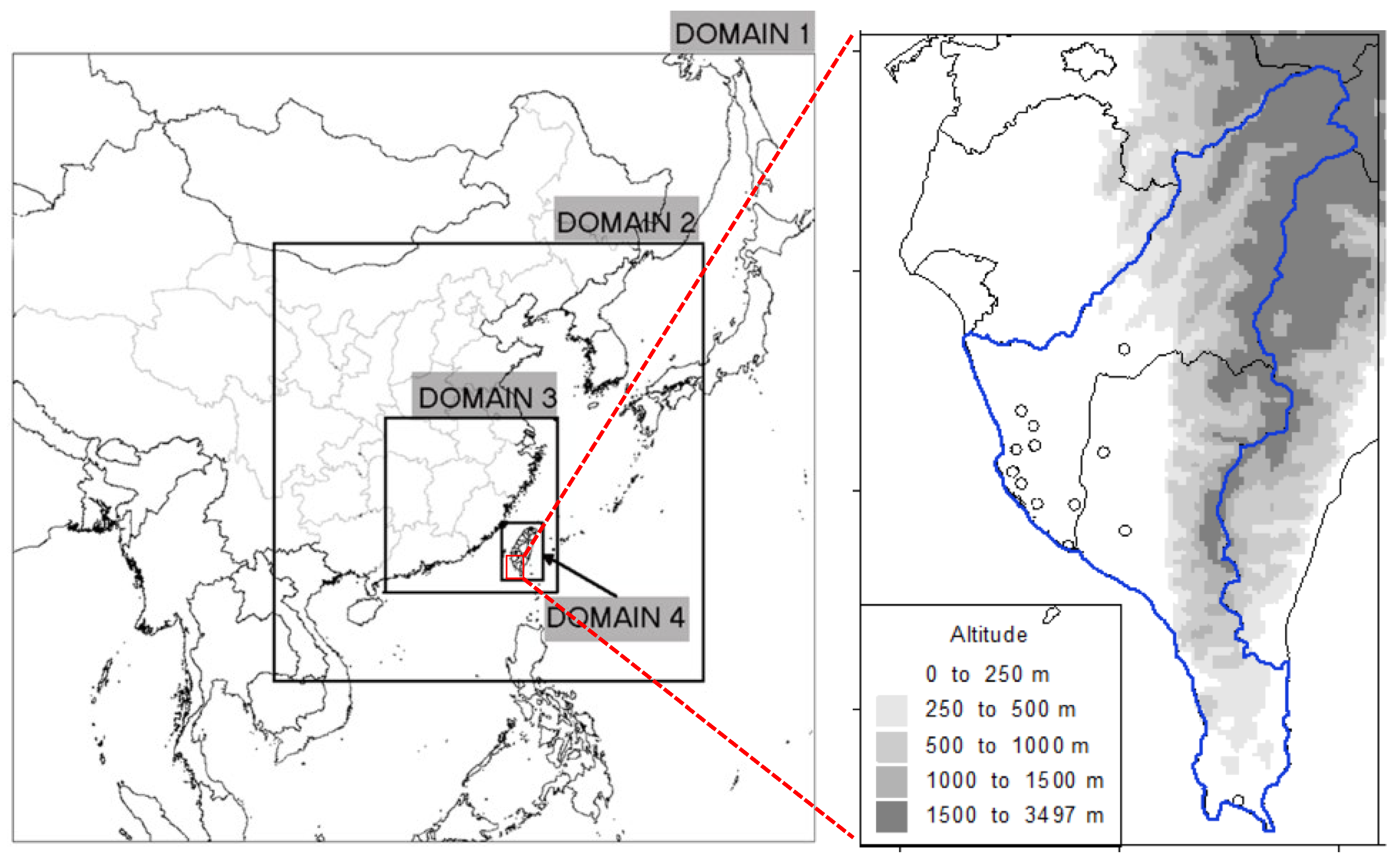
In this study, the air quality simulation system of CMAQ v5.0.2 [9] was adopted. The system was used to perform a four-level nested grid simulation. The coverage of the simulation grid is depicted in Figure 1. Domain 1 (D1) covered Greater East Asia, the scope of D2–D4 gradually decreased but the grid resolution gradually increased, and D4 covered the entirety of Taiwan. The grid resolution was 81, 27, 9, and 3 km, respectively. The simulation period was January, April, July, and October 2013, and the average result of these four months represented the annual average. The initial and boundary conditions used by the simulation system were based on the built-in data sets in the model. Therefore, this study enabled the reduction of the impact of incorrect initial conditions by several days of pre-running and enabled the reduction of the impact of faulty boundary conditions by the four-level nested simulation mentioned above. The meteorological input data for CMAQ were obtained from the WRF model’s output (Weather Research and Forecast model) [10]. Since the simulation scope covered Greater East Asia, the emission data involved in the simulation system should include the anthropogenic and biogenic emission sources in this region. As for anthropogenic emission data, the data for Taiwan anthropogenic source emissions was the 2013 base year emission data (Taiwan Emission Database System version 9.0) published by TEPA, the data for Chinese anthropogenic source emissions was from the MEIC-2012 database (Multi-resolution Emission Inventory for China) [11], and data for anthropogenic emission sources in other parts of East Asia was from the MIX database [12]. As for biogenic emission data, the hourly biogenic emissions in Taiwan were estimated using the Taiwan Biogenic Emission Inventory System [13] with meteorological data, and the hourly biogenic emissions in China and other parts of East Asia were estimated using the East Asia Biogenic Emission Inventory System [14] with meteorological data. Figure S1 illustrates the spatial distribution of pollutant emissions from D1–D4. Table S1 summarizes the CMAQ and WRF configurations that were used in this study.
2.2. Case Simulation and Offset Ratio Calculation
The base case considered emissions from all of the sources. In addition to the base case, this study also simulated the zero-emission cases of SOX, NOX, and primary PM2.5 from the point, mobile, and fugitive sources of KPAB for a total of nine control cases. The difference between the base and control cases is the impact on PM2.5 concentration by specific pollutant emissions from a specific emission source category. This simulation method is a Brute Force Method (BFM) [15,16,17]. This method and the other two methods, the Decoupled Direct Method (DDM) [18,19,20] and the Source Apportionment Technology (SAT) [21,22,23], are commonly used sensitivity analysis methods [24]. In general, the SAT cannot capture the nonlinear response of PM2.5 concentration to emissions [21], so this method was not used in this study. The DDM is not suitable for situations where the disturbance is too large [21]. The BFM is common and easy to operate, although it is more computationally demanding [24]. The response to secondary PM2.5 precursor emissions predicted by the BFM method will be greater than that predicted by the DDM method, while the response to primary PM2.5 emissions predicted by the BFM method will be similar to that predicted by the DDM method [21]. It can be inferred from this that the offset ratios of primary PM2.5 emissions for inter-source categories (mobile to point and fugitive to point) calculated by the estimation results of the DDM method should be similar to those of the BFM method, and the inter-pollutant offset ratios (SOX-to-PM2.5, NOX-to-PM2.5) calculated by the estimation results of the DDM method should be greater than those of the BFM method.
In this study, modifications of the equation proposed by Boylan and Kim [8] were made to generate the following equation, through which the sensitivity of PM2.5 concentration to specific pollutant emissions from a specific source category () can be calculated.
In which i is the station/grid, t is the emission source category (point, mobile, or fugitive source), s is the pollutant species (SOX, NOX, or primary PM2.5) emitted by the emission source category, and is the emission reduction of pollutant species s from the source category t. is the impact on the PM2.5 concentration of station/grid i by the emission reduction of pollutant species s from the source category t. The equation for the relative sensitivity (offset ratio) of different pollutant species (s2 to s1) from different emission source categories (t2 to t1) to station/grid i is expressed as follows:
For example, the reduction of point source SOX emissions can be converted to the increase of the PM2.5 emissions of point sources through the following equation, so that the PM2.5 concentration of station/grid i can remain unchanged:
The reduction of mobile source NOX emissions can be converted into the increase of the PM2.5 emissions of point sources through the following equation, so that the PM2.5 concentration of station/grid i can remain unchanged:
Finally, calculations of the different statistics of of all stations/grids were made, including maximum, minimum, and several percentile values. In addition, this study also treated all stations/grids (N) in KPAB as one to calculate the offset ratio (RCAVE) of different pollutant types (s2 to s1) from different emission source categories (t2 to t1):
Most of the air quality observation stations in Taiwan are located in densely populated areas, so the statistics for the station data can best represent most of the living areas (urban areas). There are 13 stations in KPAB, as presented in Figure 1. The statistics of the grid data were calculated based on the land cover grid of KPAB (631 grid cells in total), representing the entire air basin.
3. Results and Discussion
3.1. Base Case Simulation Results and Their Performance Evaluation Results
Figure S2 shows the spatial distribution of the annual average PM2.5 concentration in D1–D4. High PM2.5 concentrations in mainland China (D2) mainly occurred in Hebei, Shandong, Hunan, and Sichuan, which were greater than 100 μg/m3. Based on the spatial distribution of Taiwan’s annual average PM2.5 concentration (D4), the concentration on the western plain was higher than that in the eastern region. The highest concentration in the western plain of Taiwan occurred in KPAB, which could reach more than 30 μg/m3, and the concentration in other areas was mostly between 10–26 μg/m3, while the concentration in the eastern region of Taiwan, in contrast, was between 6–16 μg/m3.
Table S2 shows the quantified error analysis results of the simulated and observed PM2.5 daily average concentrations at air quality stations in KPAB. As can be seen in the table, the Mean Fractional Bias (MFB) and Mean Fractional Error (MFE) for most months met the PM2.5 simulation performance goals (the level of accuracy that is considered to be close to the best a model can be expected to achieve) proposed by Boylan and Russell [25], i.e., MFB ≤ ±30% and MFE ≤ 50%. Only the MFE in July (52%) did not meet the goal, but it still met the suggested PM2.5 simulation performance criteria (the level of accuracy that is considered to be acceptable for modeling applications) from the same article, namely MFB ≤ ±60% and MFE ≤ 75%. The Index of Agreement in each month met the standard of greater than or equal to 0.5 recommended by Hurley et al. [26]. In addition, this study also calculated the Correlation and Root Mean Square Error, the former falling between 0.56–0.71 and the latter between 10.7–17.7 μg/m3. Overall, the simulated performance of PM2.5 in January, April, July, and October 2013 should be acceptable.
3.2. Sensitivity of PM2.5 Concentrations to the Emissions of Different Pollutants from Different Source Categories over KPAB
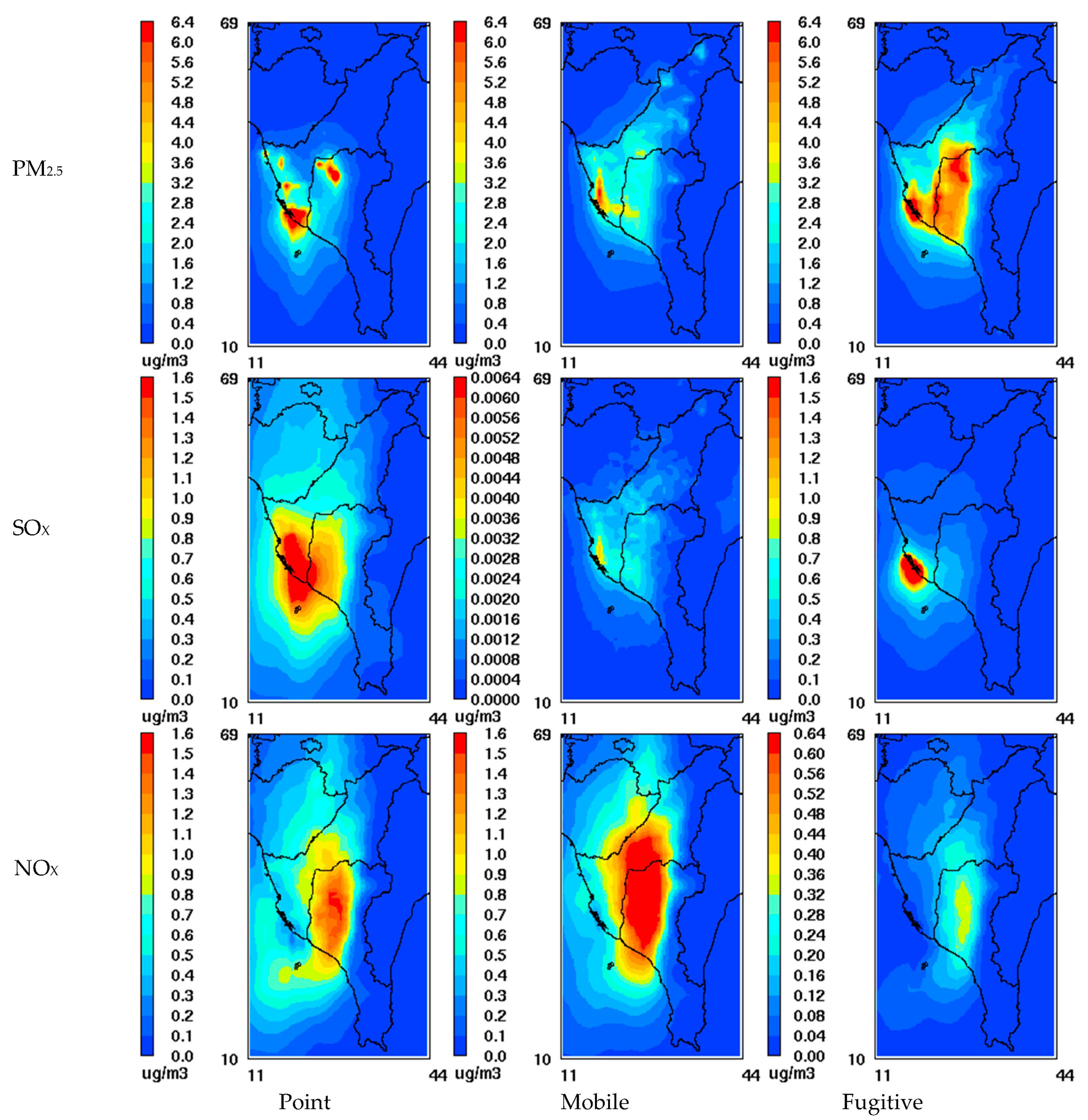
Figure 2 depicts the spatial distribution of various pollutant emissions from point, mobile, and fugitive sources in KPAB. The high emissions of SOX, NOX, and PM2.5 from point sources were mostly located in significant point sources, such as power plants and steel plants, and industrial areas. These areas were also quite close to densely populated urban areas. The significant emission locations of NOX and PM2.5 from mobile sources were primarily along highways and urban areas, and their SOX emissions were very low. The distribution range of PM2.5 emissions from fugitive sources was relatively wide, and their higher emissions appeared in densely populated urban areas, while their SOX and NOX emissions were concentrated but not high. Regarding the total emissions of pollutants, as provided in Table 1, nearly half of the PM2.5 emissions were mainly generated from fugitive sources, while point and mobile sources evenly contributed to the rest. The emissions of SOX were mainly attributed to point sources, while the emissions of NOX were particularly significant in both mobile and point sources.
The spatial distribution and quantification of the effects of various pollutants from KPAB’s point, mobile, and fugitive sources on the annual average concentration of PM2.5 are shown, respectively in Figure 3 and Table 2. Regarding the impact of primary PM2.5 emissions from emission sources, the primary PM2.5 emissions can directly affect the PM2.5 concentration without undergoing chemical reactions. Therefore, the high-impact areas were mainly located around the emission source. Moreover, as can be seen from the figure, the impact of point sources was more concentrated, whereas mobile and fugitive sources had a wider area of influence. In addition, due to the high-altitude discharge of point sources, pollutants can be transported to farther locations. Since the prevailing wind direction was northerly, there was a high-impact concentration in the southern seas of urban Kaohsiung. From the comparison of the quantified results, the station average shows that the total impact of point and fugitive source emissions ( in the table) were similar and higher than that of mobile emissions. However, when the impact was converted (divided by total emission) into the effectiveness of unit emission reduction ( in the table) for comparison, it was found that the point source was the highest and that the fugitive source was the lowest. By referring to the results of the region average, fugitive sources tended to have the highest total emission impact, and mobile sources had rather the highest effectiveness per unit emission reduction. This part of the finding indicates that reducing point source emissions should be a priority option as this led to better concentration improvements in urban areas, whereas improvements in concentration in non-urban areas relied more on reducing emissions from mobile sources.
From Figure 3, the high-impact concentration range of SOX emission was greater than that of primary PM2.5. This was because SO2 (sulfur dioxide) is a precursor of secondary PM2.5. Due to the large amount of SO2 emissions from point sources, their impact concentration was higher than both that of mobile sources and that of fugitive sources; mobile sources had a meager impact on the PM2.5 concentration because the emission was too small. By comparing the quantified results, fugitive sources had the highest unit emission reduction benefits, and point sources had the lowest ones. However, mobile and fugitive sources could only emit relatively small emissions, and the total impact concentration was insignificant, thereby making them unsuitable objects for SOX reduction.
The high impact of NOX emission on PM2.5 concentration mainly occurred in the downwind areas far away from the emission sources. That was because NH3 (ammonia) reacts with H2SO4 (sulfuric acid) first, then the remaining NH3 reacts with HNO3 (nitric acid) to form nitrate [27]. In addition, there was a large amount of NH3 emission from livestock farming in the downwind areas (Figure S1), resulting in a more significant increase in nitrate concentration in the downwind areas. Therefore, the spatial distribution of impacts of NOX emissions from the three categories of emission sources was similar. Simply stated, the high impact in this regard was expected to be near the non-urban areas, while the urban areas were relatively unaffected. Moreover, based on the obtained quantified results, the unit emission reduction benefits of the three categories of emission sources were almost the same in both the station average and the regional average. However, the emission from fugitive sources was relatively small, and the total impact concentration was insignificant, thus making them unsuitable objects for NOX reduction.
3.3. Calculation of Emission Offset Ratios for KPAB
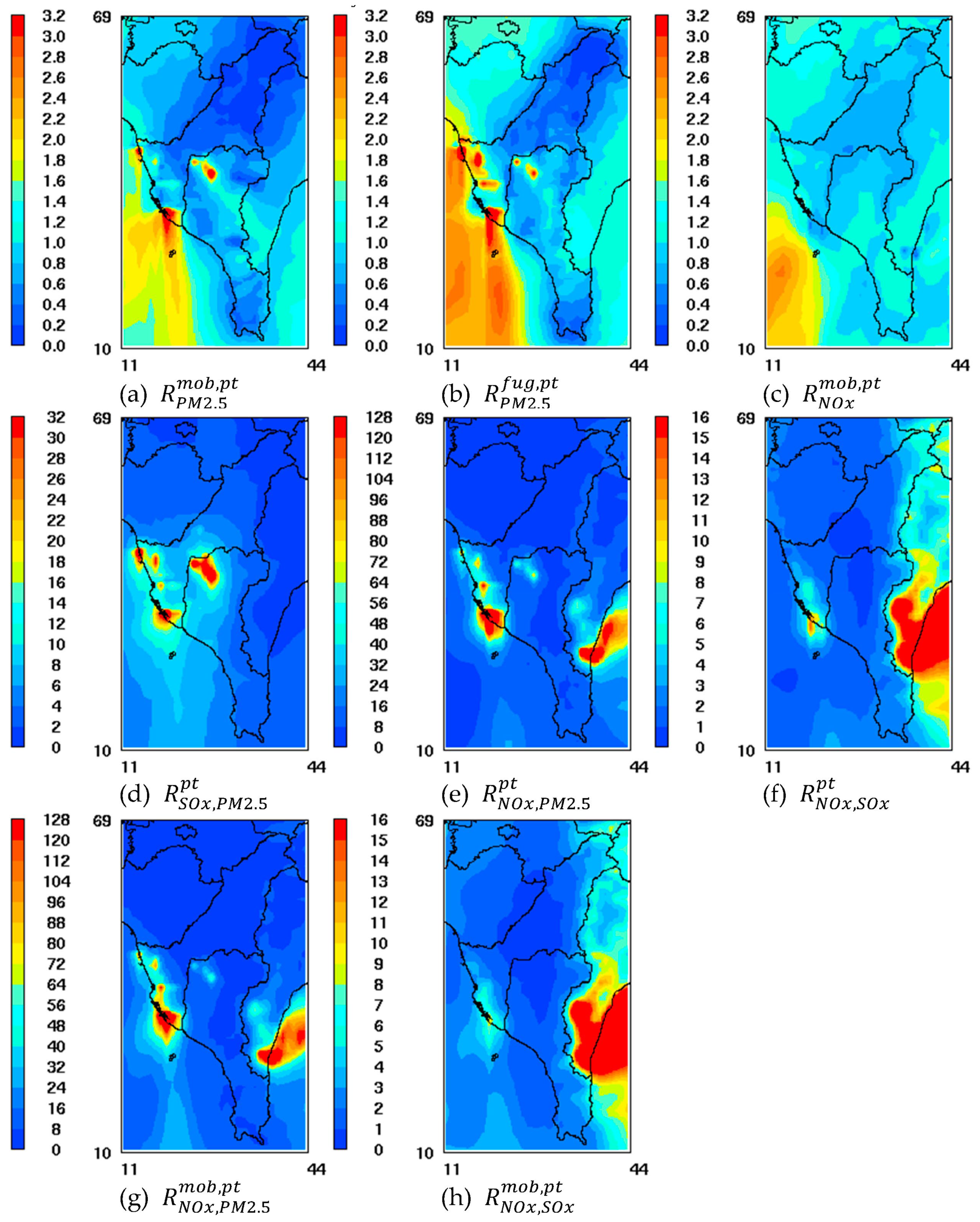
Various inter-source categories and/or inter-pollutant emission offset ratios can be calculated using Equation (2). However, it was unnecessary to calculate some offset ratios, including the emissions of the offset objects that were too low or offset objects not required by regulations. Offset objects with insignificant emissions included mobile source SOX and fugitive source SOX and NOX. The regulation is that emissions from stationary, mobile, and fugitive sources can be offset for emissions from stationary sources. Therefore, the eight needed offset ratios are listed in Figure 4 and Table 3 and Table 4.
Figure 4 shows the spatial distribution of the eight offset ratios, while Table 3 shows the distribution of the eight offset ratios within the KPAB area. It has been shown in the previous section that the region’s average benefits of unit primary PM2.5 emissions reduction from mobile and fugitive sources were both more significant than those from point sources. Therefore, as can be seen in Table 3 and Figure 4, across 75% of all the KPAB area, the offset ratios of primary PM2.5 emissions for inter-source categories (mobile to point, fugitive to point) were less than one. The ratio of mobile source NOX to point source NOX was also less than one in more than 75% of this particular area. Meanwhile, as noted in the previous section, the reduction benefit of unit primary PM2.5 emissions from point sources was significantly greater than both that of SOX and that of NOX. Moreover, the reduction benefit of SOX was greater than that of NOX. Therefore, the inter-pollutant offset ratios for the point source listed in Table 3 (SOX-to-PM2.5, NOX-to-PM2.5, NOX-to-SOX) all had an offset ratio greater than one in almost all the grids of KPAB. Among these, the NOX-to-PM2.5 ratio was the highest with a significant difference between high and low values. The NOX-to-SOX ratio was the smallest. Of the inter-source category and inter-pollutant offset ratios, mobile NOX-to-point PM2.5 ratios and mobile NOX-to-point SOX ratios had similar values and distribution to point NOX-to-point PM2.5 ratios and point NOX-to-point SOX ratios, respectively, as clearly depicted in Figure 4. This was mainly due to the similarity between the unit emission reduction benefits of point source NOX and those of mobile source NOX (Table 2).
Table 4 presents the distribution of the eight offset ratios across the stations in KPAB. In the comparison of it in Table 3, most stations were located in the high-ratio areas of KPAB. This suggests that the urban areas usually had a higher offset ratio. In contrast with this, the non-urban areas somehow had a low offset ratio. This is clearly illustrated in Figure 4. To be specific, to actively improve the PM2.5 pollution in KPAB, the offset ratios over the stations should be considered to develop the recommended offset ratios; however, to better improve both the PM2.5 pollution and the economic development, the offset ratios over KPAB should be considered to develop the recommended offset ratios. In addition, as given in Figure 4, parts of the high-value offset ratios appeared not only in the urban area but also in downwind areas further away from the emission sources, sometimes even outside KPAB. This situation usually occurred during the inter-pollutant offsets involving NOX, such as point NOX-to-point PM2.5, point NOX-to-point SOX, mobile NOX-to-point PM2.5, and mobile NOX-to-point SOX (Figure 4e–h). That was because the impact of PM2.5 concentration caused by NOX emission in downwind areas further away from the emission sources was significantly lower than both that of the primary PM2.5 emissions and that of the SOX emissions. This part of the results is consistent with that derived from the study conducted by Boylan and Kim [8].
In Table 3 and Table 4, various statistics for can be selected to set the preferred offset ratios for KPAB. Generally, the higher the selected percentile, the more conducive to the improvement of PM2.5 concentration. However, we should pay attention to the exchangeability between the pollutant emission offset ratios. For example, if the column 75th percentile of Table 4 was selected, the point SOX-to-point PM2.5 offset ratio was about 12, and the point NOX-to-point PM2.5 offset ratio was about 46, and the point NOX-to-point SOX offset ratio should be set at 3.8 (46/12), instead of 4.5, to make the offset emissions of the three pollutants exchangeable. Another method for calculating the offset ratio in this study was to treat all stations/grids as one, which was calculated according to Formula (5), and the results are listed in column CAVE of Table 3 and Table 4. This method does not have the hassle of equivalent substitution, and most of the calculated offset ratios were higher than the median values or even the 75th percentile values. It means that the use of RCAVE could make the PM2.5 concentration of more than 50% or even more than 75% of the areas/stations in KPAB not deteriorate or even improve. If RCAVE was selected to set the offset ratios for KPAB, even the conservative offset ratios (ratio of point SOX/NOX to point PM2.5 = 20/60) were significantly lower than the original offset principles (ratio of SOX/NOX to PM2.5 = 40/200) in Taiwan. This result indicates that the original offset principles did need to be modified. In fact, the original offset principles have been revised based on the results of this study.
4. Conclusions
In this study, the air quality simulation system was adopted to estimate the impact and the offset ratios of the three pollutants (PM2.5, SOX, and NOX) emissions from the three source categories (point, mobile, and fugitive) in KPAB, a heavy industrial area. After excluding the emissions of offset objects that were too low or the offset objects that were not required by regulations, there were eight remaining inter-source categories and/or inter-pollutant emission offsets. In KPAB, because point sources are located in close proximity to densely populated urban areas, coupled with the differences in the chemical reaction characteristics of different pollutants to form PM2.5 in the atmosphere, the impact and the offset ratios were estimated as follows. (1) The impact of unit primary PM2.5 emission from point sources on urban PM2.5 concentration was higher than both that of mobile sources and that of fugitive sources, while its impact on non-urban PM2.5 concentration was lower than both that of mobile sources and that of fugitive sources. This result makes the offset ratios (RCAVE) of mobile PM2.5-to-point PM2.5 and fugitive PM2.5-to-point PM2.5 both greater than one in urban areas (1.3 and 2.0, respectively) and both less than one in non-urban areas. (2) The impact of unit primary PM2.5 emission from point sources on urban and non-urban PM2.5 concentrations was significantly higher than that of unit SOX emission and that of unit NOX emission. This result makes the offset ratios of point SOX-to-point PM2.5 and point NOX-to-point PM2.5 significantly greater than one, especially the offset ratios in urban areas (20 and 60) were significantly higher than those in non-urban areas by more than 2–4 times. (3) The impact of unit NOX emission from point sources on PM2.5 concentrations whether in urban and non-urban areas was similar to that of unit NOX emission from line sources. This result, no matter in urban or non-urban areas, makes the offset ratio of mobile NOX-to-point NOX close to one and makes the offset ratios of point NOX-to-point PM2.5 and mobile NOX-to-point PM2.5 close to each other.
Supplementary Materials
The following supporting information can be downloaded at: https://www.mdpi.com/article/10.3390/atmos14040748/s1, Table S1: Selection of CMAQ and WRF configuration options for this study; Table S2: Quantified error analysis results of the simulated and observed PM2.5 daily average concentrations at air quality stations in KPAB; Figure S1: Spatial distribution of various pollutant emissions in D1–D4 for the base case in the year of 2013; Figure S2: Spatial distribution of the annual average concentration (average of January, April, July, and October) of PM2.5 in D1–D4 for the base case in the year of 2013.
Author Contributions
Conceptualization, T.-F.C. and K.-H.C.; methodology, T.-F.C. and B.-Y.C.; Software, T.-F.C. and B.-Y.C.; writing—original draft, T.-F.C. and B.-Y.C.; writing—reviewing and editing, T.-F.C. and K.-H.C. All authors have read and agreed to the published version of the manuscript.
Funding
This research was supported by the Taiwan Ministry of Science and Technology (MOST-111-2221-E-224-009) and the Taiwan Environmental Protection Administration (EPA-112-F-095).
Institutional Review Board Statement
Not applicable.
Informed Consent Statement
Not applicable.
Data Availability Statement
All the data are present in the manuscript.
Acknowledgments
This research was carried out with the support from the Taiwan Ministry of Science and Technology (MOST-111-2221-E-224-009) and the Taiwan Environmental Protection Administration (EPA-112-F-095).
Conflicts of Interest
The authors declare no conflict of interest.
References
- TEPA. Total Air Pollutants Quantity Control Plans for Kaohsiung-Pingtung Area. In Executive Yuan Gazette; Taiwan Environmental Protection Administration: Taipei, Taiwan, 2015; Volume 21. (In Chinese) [Google Scholar]
- TEPA. Air Quality Annual Report of R.O.C. (Taiwan), 2021; Taiwan Environmental Protection Administration: Taipei, Taiwan, 2022. (In Chinese)
- TEPA. Air Pollution Control Act (Amendment). In Presidential Office Gazette; Taiwan Environmental Protection Administration: Taipei, Taiwan, 2018. (In Chinese) [Google Scholar]
- TEPA. Offset Principles for the Increased Air Pollutant Emissions Caused by Development Activities. In Executive Yuan Gazette; Taiwan Environmental Protection Administration: Taipei, Taiwan, 2009; Volume 28. (In Chinese) [Google Scholar]
- TEPA. Offset Principles for the Increased Air Pollutant Emissions Caused by Development Activities (Amendment). In Executive Yuan Gazette; Taiwan Environmental Protection Administration: Taipei, Taiwan, 2022; Volume 15. (In Chinese) [Google Scholar]
- USEPA. Implementation of the New Source Review (NSR) Program for Particulate Matter Less Than 2.5 Micrometers (PM2.5). In Federal Register; U.S. Environmental Protection Agency: Research Triangle Park, NC, USA, 2008; Volume 73, pp. 28321–28350. [Google Scholar]
- NACAA. PM2.5 Modeling Implementation for Projects Subject to National Ambient Air Quality Demonstration Requirements Pursuant to New Source Review: Report from NACAA PM2.5 Modeling Implementation Workgroup; National Association of Clean Air Agencies: Washington, DC, USA, 2011. [Google Scholar]
- Boylan, J.; Kim, B. Development of PM2 5 interpollutant trading ratios. In Proceedings of the 2012 Community Modeling & Analysis System (CMAS) Conference, Chapel Hill, NC, USA, 16 October 2012. [Google Scholar]
- USEPA. CMAQ Version 5.0.2. Available online: https://zenodo.org/record/1079898 (accessed on 2 June 2015).
- Skamarock, W.C.; Klemp, J.B.; Dudhia, J.; Gill, D.O.; Barker, D.M.; Duda, M.G.; Huang, X.Y.; Wang, W.; Powers, J.G. A Description of the Advanced Research WRF Version 3 NCAR/TN-475+STR; National Center for Atmospheric Research: Boulder, CO, USA, 2008. [Google Scholar]
- Zheng, B.; Tong, D.; Li, M.; Liu, F.; Hong, C.; Geng, G.; Li, H.; Li, X.; Peng, L.; Qi, J.; et al. Trends in China’s anthropogenic emissions since 2010 as the consequence of clean air actions. Atmos. Chem. Phys. 2018, 18, 14095–14111. [Google Scholar] [CrossRef]
- Li, M.; Zhang, Q.; Kurokawa, J.I.; Woo, J.H.; He, K.; Lu, Z.; Ohara, T.; Song, Y.; Streets, D.G.; Carmichael, G.R.; et al. MIX: A mosaic Asian anthropogenic emission inventory under the international collaboration framework of the MICS-Asia and HTAP. Atmos. Chem. Phys. 2017, 17, 935–963. [Google Scholar] [CrossRef]
- Chang, K.H.; Yu, J.Y.; Chen, T.F.; Lin, Y.P. Estimating Taiwan biogenic VOC emission: Leaf energy balance consideration. Atmos. Environ. 2009, 43, 5092–5100. [Google Scholar] [CrossRef]
- Chen, T.F.; Chen, C.H.; Yu, J.Y.; Lin, Y.B.; Chang, K.H. Estimation of biogenic VOC emissions in East Asia with new emission factors and leaf energy balance considerations. J. Innov. Technol. 2020, 2, 61–72. [Google Scholar]
- Streets, D.G.; Fu, J.S.; Jang, C.J.; Hao, J.; He, K.; Tang, X.; Zhang, Y.; Wang, Z.; Li, Z.; Zhang, Q.; et al. Air quality during the 2008 Beijing Olympic Games. Atmos. Environ. 2007, 41, 480–492. [Google Scholar] [CrossRef]
- Xing, J.; Zhang, Y.; Wang, S.; Liu, X.; Cheng, S.; Zhang, Q.; Chen, Y.; Streets, D.G.; Jang, C.; Hao, J.; et al. Modeling study on the air quality impacts from emission reductions and atypical meteorological conditions during the 2008 Beijing Olympics. Atmos. Environ. 2011, 45, 1786–1798. [Google Scholar] [CrossRef]
- Lee, D.; Choi, J.-Y.; Myoung, J.; Kim, O.; Park, J.; Shin, H.-J.; Ban, S.-J.; Park, H.-J.; Nam, K.-P. Analysis of a severe PM2.5 episode in the Seoul Metropolitan area in South Korea from 27 February to 7 March 2019: Focused on estimation of domestic and foreign contribution. Atmosphere 2019, 10, 756. [Google Scholar] [CrossRef]
- Cohan, D.S.; Hakami, A.; Hu, Y.; Russell, A.G. Nonlinear response of ozone to emissions: Source apportionment and sensitivity analysis. Environ. Sci. Technol. 2005, 39, 6739–6748. [Google Scholar] [CrossRef] [PubMed]
- Itahashi, S.; Uno, I.; Kim, S. Source contributions of sulfate aerosol over East Asia estimated by CMAQ-DDM. Environ. Sci. Technol. 2012, 46, 6733–6741. [Google Scholar] [CrossRef] [PubMed]
- Yu, S.; Su, F.; Yin, S.; Wang, S.; Xu, R.; He, B.; Fan, X.; Yuan, M.; Zhang, R. Characterization of ambient volatile organic compounds, source apportionment, and the ozone–NOx–VOC sensitivities in a heavily polluted megacity of central China: Effect of sporting events and emission reductions. Atmos. Chem. Phys. 2021, 21, 15239–15257. [Google Scholar] [CrossRef]
- Koo, B.; Wilson, G.M.; Morris, P.E.; Dunker, A.M.; Yarwood, G. Comparison of source apportionment and sensitivity analysis in a particulate matter air quality model. Environ. Sci. Technol. 2009, 43, 6669–6675. [Google Scholar] [CrossRef] [PubMed]
- Kwok, R.H.F.; Napelenok, S.L.; Baker, K.R. Implementation and evaluation of PM2.5 source contribution analysis in a photochemical model. Atmos. Environ. 2013, 80, 398–407. [Google Scholar] [CrossRef]
- Siouti, E.; Skyllakou, K.; Kioutsioukis, I.; Patoulias, D.; Fouskas, G.; Pandis, S.N. Development and application of the SmartAQ high-resolution air quality and source apportionment forecasting system for European urban areas. Atmosphere 2022, 13, 1693. [Google Scholar] [CrossRef]
- Cohan, D.S.; Napelenok, S.L. Air quality response modeling for decision support. Atmosphere 2011, 2, 407–425. [Google Scholar] [CrossRef]
- Boylan, J.W.; Russell, A.G. PM and light extinction model performance metrics, goals, and criteria for three-dimensional air quality models. Atmos. Environ. 2006, 40, 4946–4959. [Google Scholar] [CrossRef]
- Hurley, P.; Blockley, A.; Rayner, K. Verification of a prognostic meteorological and air pollution model for year-long predictions in the Kwinana region of Western Australia. Atmos. Environ. 2001, 35, 1871–1880. [Google Scholar] [CrossRef]
- Seinfeld, J.H.; Pandis, S.N. Atmospheric Chemistry and Physics: From Air Pollution to Climate Change, 3rd ed.; John Wiley & Sons: Hoboken, NJ, USA, 2016. [Google Scholar]
Figure 1.
Configuration of four-level nesting domains (left picture), KPAB district (area surrounded by blue frame in right picture), and air quality monitoring locations within KPAB (circles in right picture).
Figure 1.
Configuration of four-level nesting domains (left picture), KPAB district (area surrounded by blue frame in right picture), and air quality monitoring locations within KPAB (circles in right picture).

Figure 2.
Spatial distribution of various pollutant emissions from point, mobile, and fugitive sources in KPAB.
Figure 2.
Spatial distribution of various pollutant emissions from point, mobile, and fugitive sources in KPAB.

Figure 3.
Spatial distribution of the influence of various pollutant emissions from point, mobile, and fugitive sources in KPAB on PM2.5 concentrations (μg/m3).
Figure 3.
Spatial distribution of the influence of various pollutant emissions from point, mobile, and fugitive sources in KPAB on PM2.5 concentrations (μg/m3).

Figure 4.
Spatial distribution of the eight needed offset ratios, including (a) mobile PM2.5-to-point PM2.5 ratio, (b) fugitive PM2.5-to-point PM2.5 ratio, (c) mobile NOX-to-point NOX ratio, (d) point SOX-to-point PM2.5 ratio, (e) point NOX-to-point PM2.5 ratio, (f) point NOX-to-point SOX ratio, (g) mobile NOX-to-point PM2.5 ratio, and (h) mobile NOX-to-point SOX ratio.


Table 1.
Total emissions of pollutants from point, mobile, and fugitive sources in KPAB (103 ton/year).
Table 1.
Total emissions of pollutants from point, mobile, and fugitive sources in KPAB (103 ton/year).
| t= | Point | Mobile | Fugitive | |
|---|---|---|---|---|
| s | ||||
| PM2.5 | 2.69 | 2.53 | 5.11 | |
| SOX | 16.4 | 0.02 | 0.33 | |
| NOX | 22.8 | 27.4 | 3.14 |
Table 2.
Quantification of the impact empty( ) and sensitivity ( ) of various pollutant emissions from point, mobile, and fugitive sources ( ) in KPAB on PM2.5 concentrations in KPAB.
Table 2.
Quantification of the impact empty( ) and sensitivity ( ) of various pollutant emissions from point, mobile, and fugitive sources ( ) in KPAB on PM2.5 concentrations in KPAB.
| a= | All Station Average (N = 13) | Region Average (N = 631) | |||||
|---|---|---|---|---|---|---|---|
| t= | Point | Mobile | Fugitive | Point | Mobile | Fugitive | |
(µg/m3) | 4.33 | 3.14 | 4.18 | 0.91 | 1.21 | 1.90 | |
(µg/m3/103 ton) | 1.61 | 1.24 | 0.82 | 0.34 | 0.48 | 0.37 | |
(µg/m3) | 1.38 | 0.0023 | 0.61 | 0.57 | 0.0009 | 0.18 | |
(µg/m3/103 ton) | 0.084 | 0.13 | 1.86 | 0.035 | 0.050 | 0.56 | |
(µg/m3) | 0.61 | 0.83 | 0.092 | 0.52 | 0.73 | 0.10 | |
(µg/m3/103 ton) | 0.027 | 0.030 | 0.029 | 0.023 | 0.027 | 0.033 | |
, , is taken from Table 1, s = PM2.5, SOX, or NOX.
Table 3.
Distribution of offset ratios over KPAB.
| Statistic (a=) | All Grid Cells (N = 631) | |||||
|---|---|---|---|---|---|---|
| Min | Median | 75th Percentile | 90th Percentile | Max | CAVE | |
| 0.01 | 0.53 | 0.80 | 1.06 | 8.51 | 0.71 | |
| 0.07 | 0.62 | 0.89 | 1.35 | 9.84 | 0.91 | |
| 0.57 | 0.86 | 0.98 | 1.07 | 1.79 | 0.86 | |
| 0.94 | 4.81 | 8.53 | 12.71 | 85.64 | 9.73 | |
| 2.72 | 8.48 | 11.87 | 29.67 | 719.08 | 14.81 | |
| 0.80 | 1.84 | 2.78 | 4.46 | 13.90 | 1.52 | |
| 2.16 | 7.72 | 10.86 | 28.79 | 673.13 | 12.71 | |
| 0.52 | 1.65 | 2.53 | 3.90 | 9.30 | 1.31 | |
, , , , , , .
Table 4.
Distribution of offset ratios over the stations in KPAB.
| Statistic (a=) | All Stations (N = 13) | |||||
|---|---|---|---|---|---|---|
| Min | Median | 75th Percentile | 92nd Percentile | Max | CAVE | |
| 0.35 | 0.61 | 1.01 | 1.73 | 7.99 | 1.30 | |
| 0.38 | 1.04 | 1.55 | 2.53 | 9.09 | 1.97 | |
| 0.58 | 0.95 | 1.00 | 1.44 | 1.48 | 0.88 | |
| 3.05 | 10.07 | 11.65 | 18.76 | 72.65 | 19.17 | |
| 6.05 | 40.91 | 45.32 | 101.18 | 651.55 | 60.33 | |
| 0.85 | 4.00 | 4.54 | 7.76 | 8.97 | 3.15 | |
| 5.35 | 40.96 | 64.88 | 97.09 | 618.05 | 53.28 | |
| 0.52 | 4.24 | 5.17 | 6.69 | 8.51 | 2.78 | |
, , , , , , .
Disclaimer/Publisher’s Note: The statements, opinions and data contained in all publications are solely those of the individual author(s) and contributor(s) and not of MDPI and/or the editor(s). MDPI and/or the editor(s) disclaim responsibility for any injury to people or property resulting from any ideas, methods, instructions or products referred to in the content. |
© 2023 by the authors. Licensee MDPI, Basel, Switzerland. This article is an open access article distributed under the terms and conditions of the Creative Commons Attribution (CC BY) license (https://creativecommons.org/licenses/by/4.0/).
Share and Cite
MDPI and ACS Style
Chen, T.-F.; Chen, B.-Y.; Chang, K.-H. Simulation and Estimation of the Inter-Source Category and/or Inter-Pollutant Emission Offset Ratios for a Heavy Industry City. Atmosphere 2023, 14, 748. https://doi.org/10.3390/atmos14040748
AMA Style
Chen T-F, Chen B-Y, Chang K-H. Simulation and Estimation of the Inter-Source Category and/or Inter-Pollutant Emission Offset Ratios for a Heavy Industry City. Atmosphere. 2023; 14(4):748. https://doi.org/10.3390/atmos14040748
Chicago/Turabian StyleChen, Tu-Fu, Bo-Yan Chen, and Ken-Hui Chang. 2023. "Simulation and Estimation of the Inter-Source Category and/or Inter-Pollutant Emission Offset Ratios for a Heavy Industry City" Atmosphere 14, no. 4: 748. https://doi.org/10.3390/atmos14040748
Note that from the first issue of 2016, this journal uses article numbers instead of page numbers. See further details here.