
Passive Hydrocarbon Sampling in a Shale Oil and Gas Production Area Shows Spatially Heterogeneous Air Toxics Exposure Based on Type and Proximity to Emission Sources


Abstract
:1. Introduction
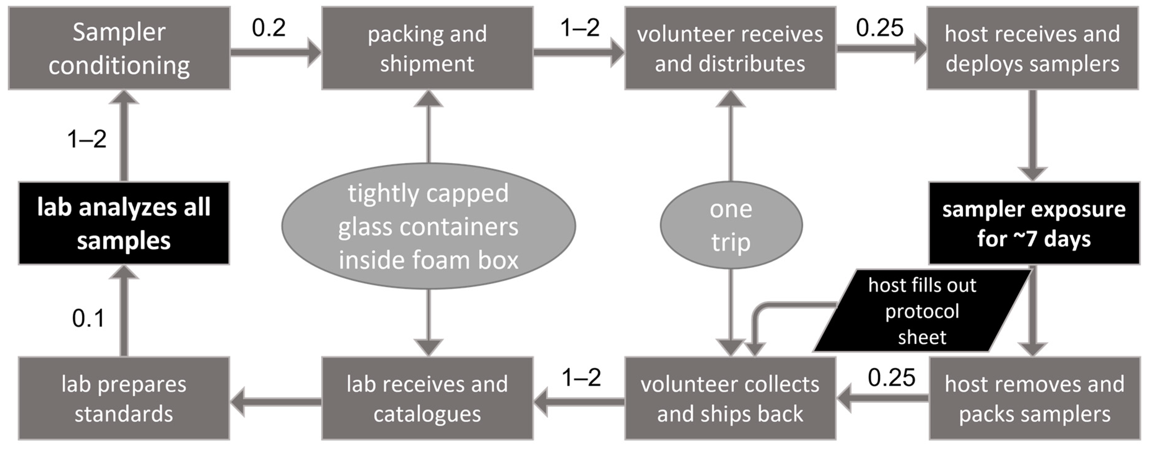
2. Methods
2.1. Study Sites
2.2. Sample Analysis
2.3. Auxiliary Data
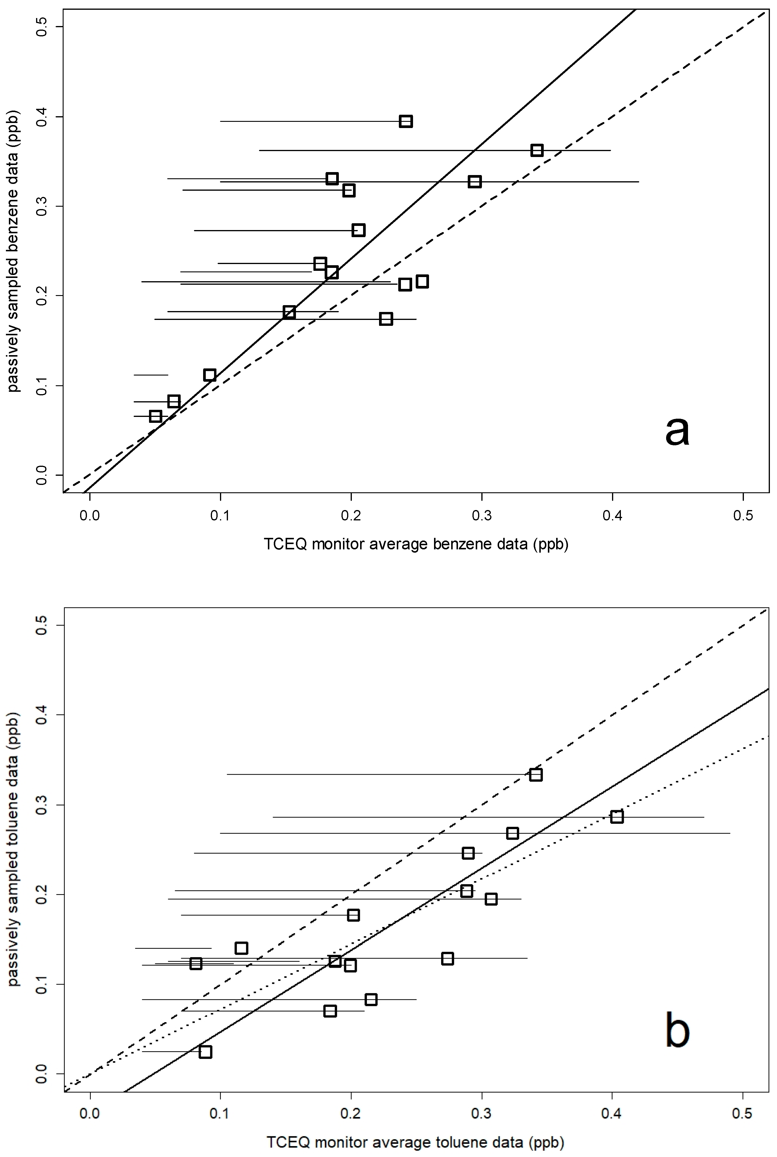
3. NMHC Validation Measurements
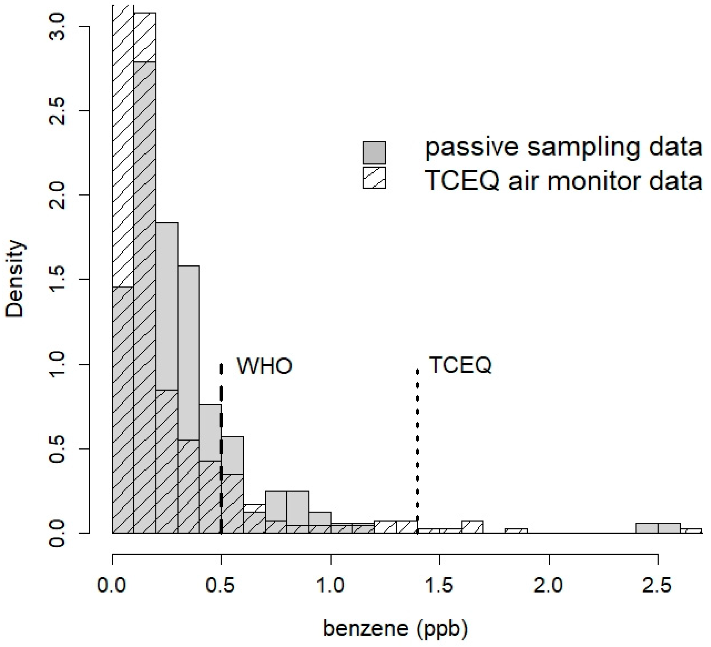
4. Ambient Exposure Observations
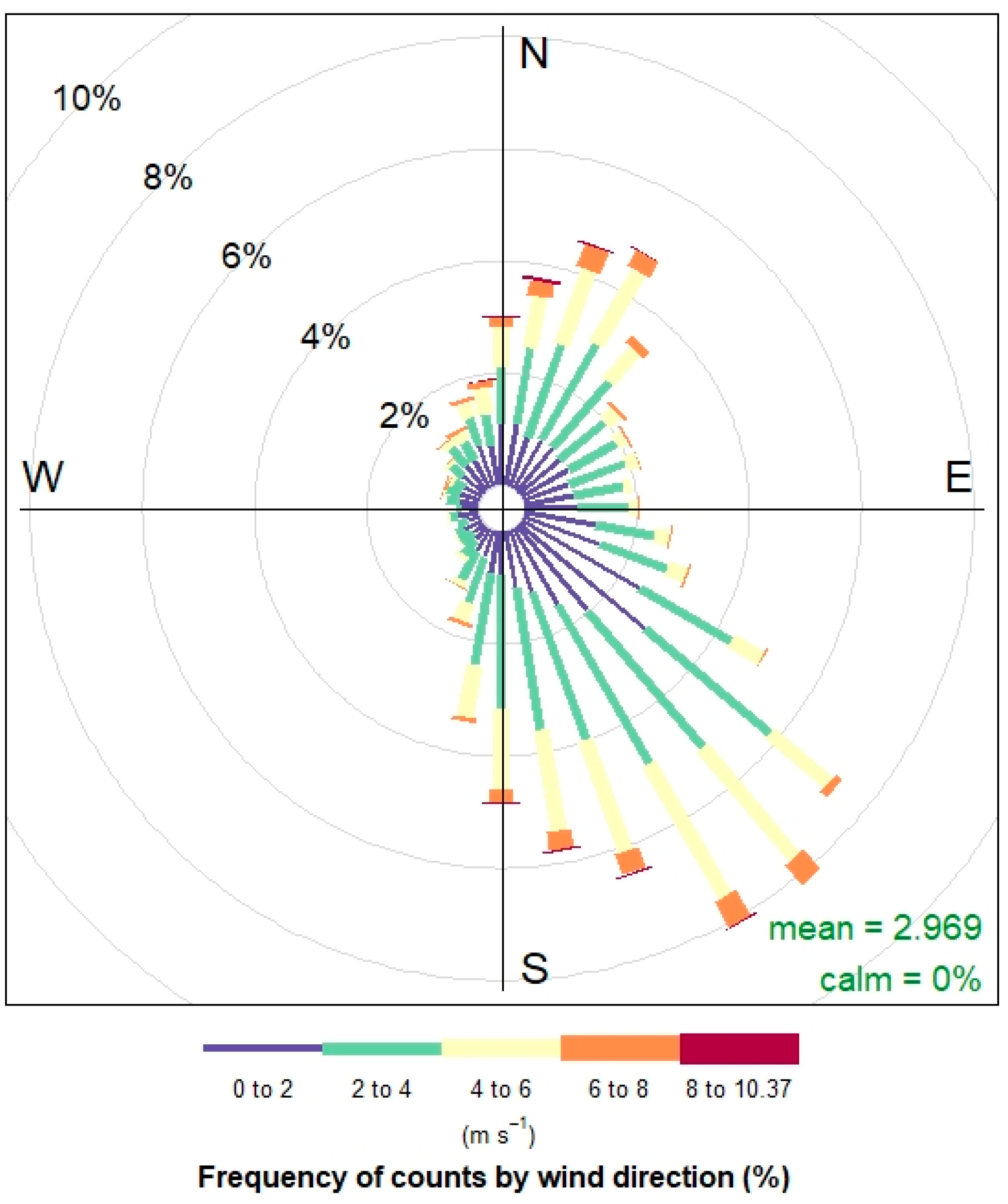
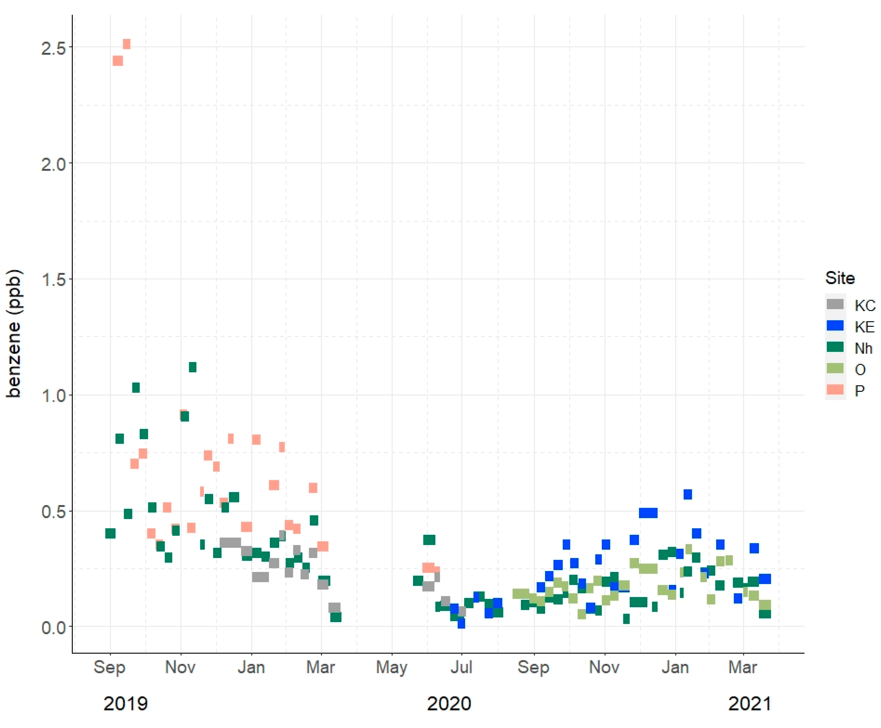
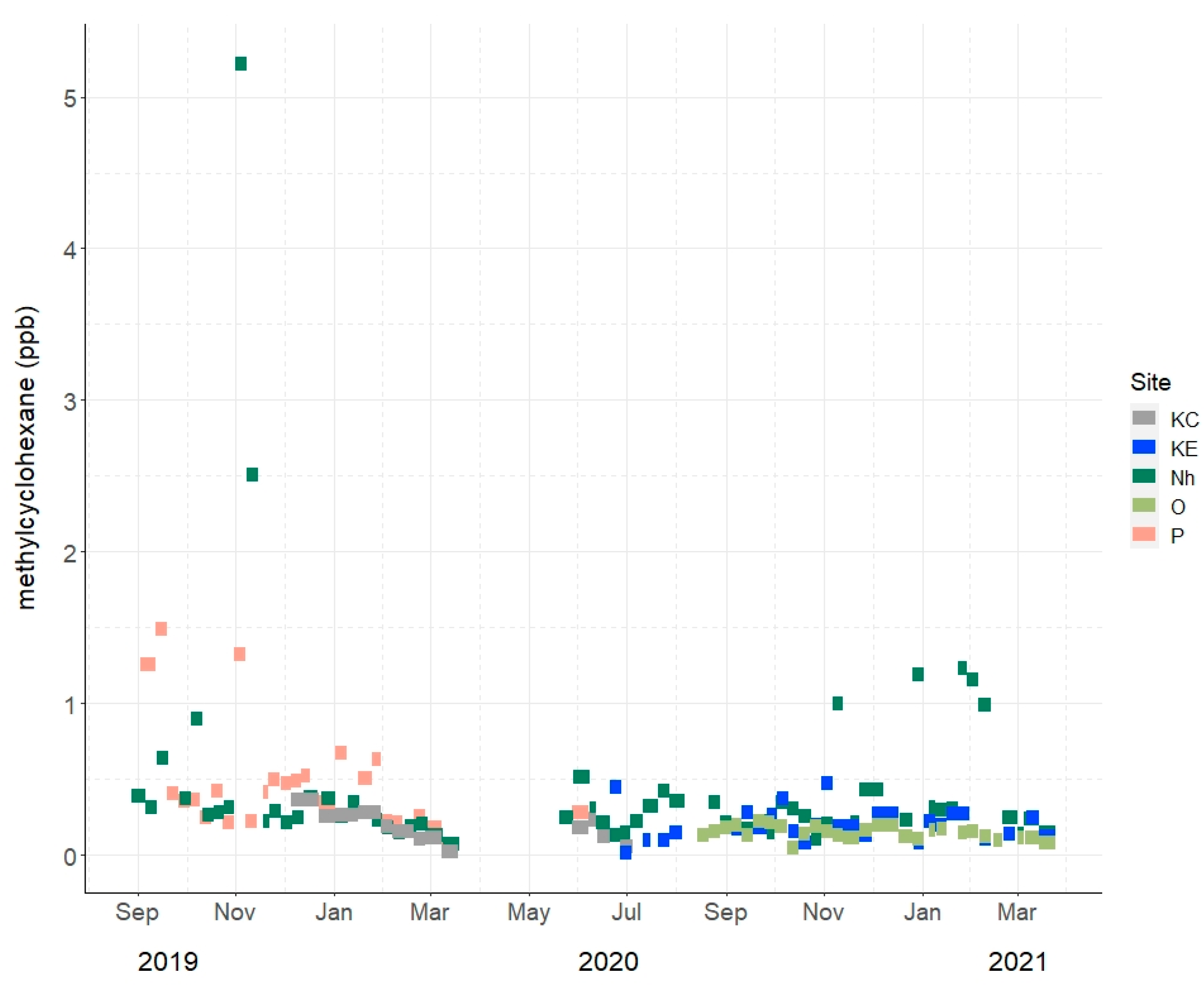
4.1. General Features
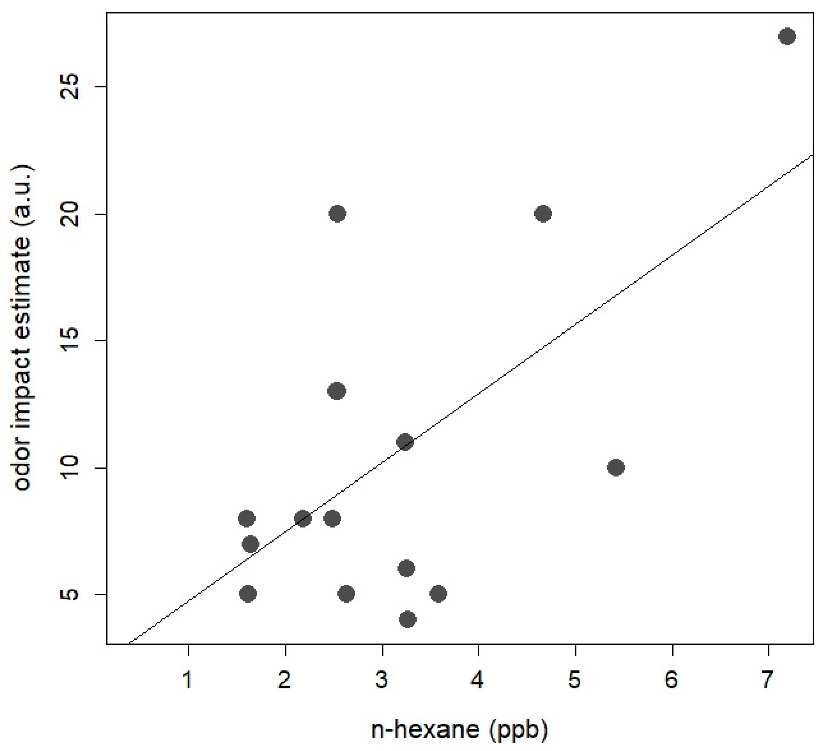
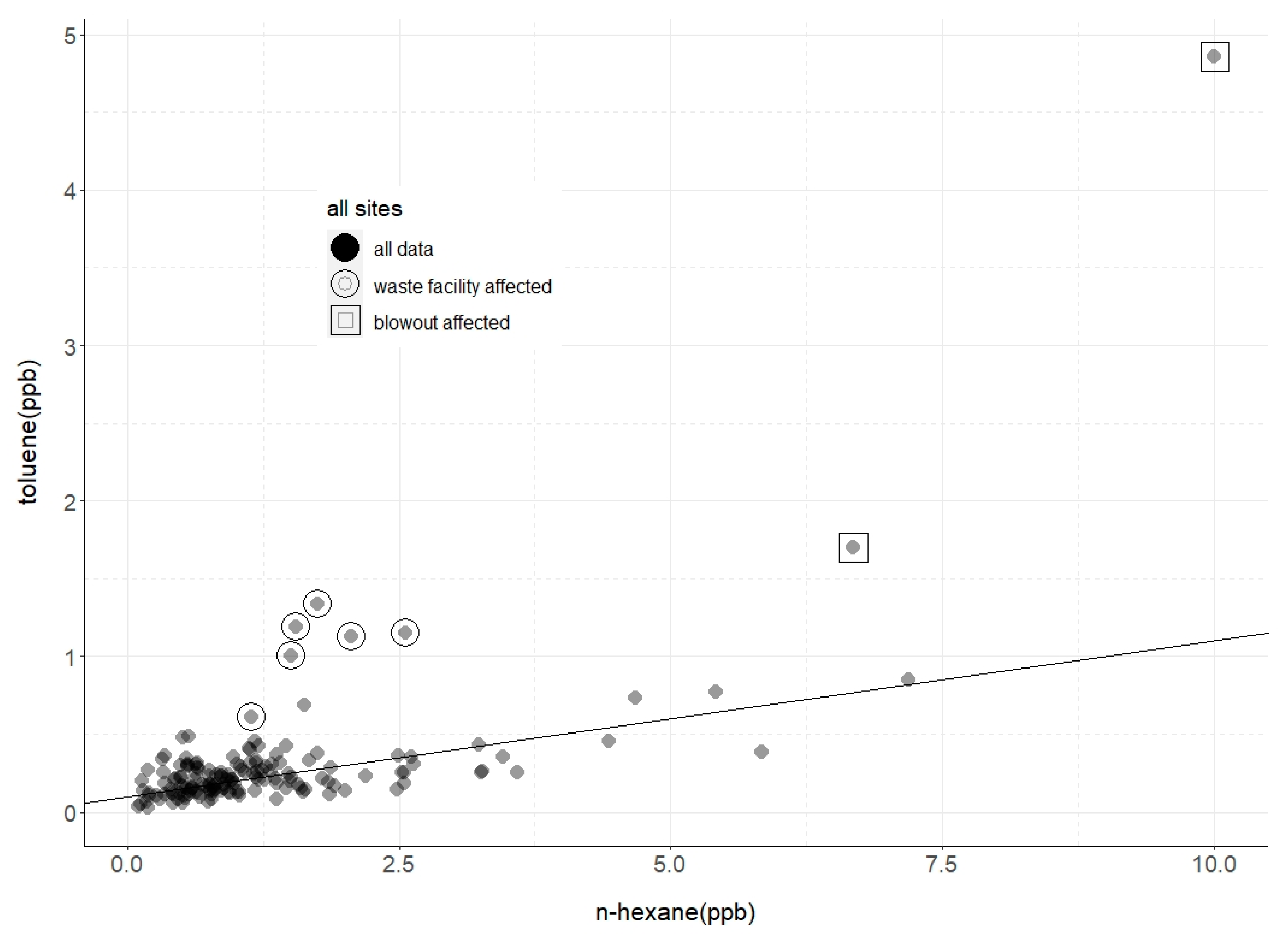
4.2. Concentration Anomalies
5. Discussion
6. Conclusions
Author Contributions
Funding
Data Availability Statement
Acknowledgments
Conflicts of Interest
References
- Allen, D.T. Emissions from oil and gas operations in the United States and their air quality implications. J. Air Waste Manag. Assoc. 2016, 66, 549–575. [Google Scholar] [CrossRef] [PubMed]
- Kanfar, M.S. Comparison of Empirical Decline Curve Analysis for Shale Wells. Master’s Thesis, Texas A&M University, College Station, TX, USA, 2013. [Google Scholar]
- Wachtmeister, H.; Lund, L.; Aleklett, K.; Höök, M. Production Decline Curves of Tight Oil Wells in Eagle Ford Shale. Nat. Resour. Res. 2017, 26, 365–377. [Google Scholar] [CrossRef]
- Braun, B. Fracking. In Keywords in Radical Geography: Antipode at 50; Wiley: Hoboken, NJ, USA, 2019; pp. 128–133. [Google Scholar]
- Murray, J.W. Limitations of Oil Production to the IPCC Scenarios: The New Realities of US and Global Oil Production. Biophys. Econ. Resour. Qual. 2016, 1, 13. [Google Scholar] [CrossRef]
- Caretta, M.A.; Carlson, E.B.; Hood, R.; Turley, B. From a rural idyll to an industrial site: An analysis of hydraulic fracturing energy sprawl in Central Appalachia. J. Land Use Sci. 2021, 16, 382–397. [Google Scholar] [CrossRef]
- da Costa, D.M.B.; Jesus, J.; Branco, D.C.; Danko, A.; Fiúza, A. Extensive review of shale gas environmental impacts from scientific literature (2010–2015). Environ. Sci. Pollut. Res. 2017, 24, 14579–14594. [Google Scholar] [CrossRef]
- Jones, N.F.; Pejchar, L.; Kiesecker, J.M. The Energy Footprint: How Oil, Natural Gas, and Wind Energy Affect Land for Biodiversity and the Flow of Ecosystem Services. Bioscience 2015, 65, 290–301. [Google Scholar] [CrossRef]
- Knighton, W.B.; Herndon, S.C.; Franklin, J.F.; Wood, E.C.; Wormhoudt, J.; Brooks, W.; Fortner, E.C.; Allen, D.T. Direct measurement of volatile organic compound emissions from industrial flares using real-time online techniques: Proton Transfer Reaction Mass Spectrometry and Tunable Infrared Laser Differential Absorption Spectroscopy. Ind. Eng. Chem. Res. 2012, 51, 12674–12684. [Google Scholar] [CrossRef]
- Marrero, J.E.; Townsend-Small, A.; Lyon, D.R.; Tsai, T.R.; Meinardi, S.; Blake, D.R. Estimating Emissions of Toxic Hydrocarbons from Natural Gas Production Sites in the Barnett Shale Region of Northern Texas. Environ. Sci. Technol. 2016, 50, 10756–10764. [Google Scholar] [CrossRef]
- Pétron, G.; Karion, A.; Sweeney, C.; Miller, B.; Montzka, S.; Frost, G.J.; Trainer, M.; Tans, P.P.; Andrews, A.; Kofler, J.; et al. A new look at methane and nonmethane hydrocarbon emissions from oil and natural gas operations in the Colorado Denver-Julesburg Basin. J. Geophys. Res. Atmos. 2014, 119, 6836–6852. [Google Scholar] [CrossRef]
- Lyon, D.R.; Alvarez, R.A.; Zavala-Araiza, D.; Brandt, A.R.; Jackson, R.B.; Hamburg, S.P. Aerial Surveys of Elevated Hydrocarbon Emissions from Oil and Gas Production Sites. Environ. Sci. Technol. 2016, 50, 4877–4886. [Google Scholar] [CrossRef]
- Allen, D.T.; Cardoso-Saldaña, F.J.; Kimura, Y. Variability in Spatially and Temporally Resolved Emissions and Hydrocarbon Source Fingerprints for Oil and Gas Sources in Shale Gas Production Regions. Environ. Sci. Technol. 2017, 51, 12016–12026. [Google Scholar] [CrossRef] [PubMed]
- Roest, G.; Schade, G. Quantifying alkane emissions in the Eagle Ford Shale using boundary layer enhancement. Atmos. Meas. Tech. 2017, 17, 11163–11176. [Google Scholar] [CrossRef]
- Rossabi, S.; Hueber, J.; Wang, W.; Milmoe, P.; Helmig, D. Spatial distribution of atmospheric oil and natural gas volatile organic compounds in the Northern Colorado Front Range. Elem. Sci. Anthr. 2021, 9, 36. [Google Scholar] [CrossRef]
- Dalsøren, S.B.; Myhre, G.; Hodnebrog, Ø.; Myhre, C.L.; Stohl, A.; Pisso, I.; Schwietzke, S.; Höglund-Isaksson, L.; Helmig, D.; Reimann, S.; et al. Discrepancy between simulated and observed ethane and propane levels explained by underestimated fossil emissions. Nat. Geosci. 2018, 11, 178–184. [Google Scholar] [CrossRef]
- Ghosh, B. Impact of Changes in Oil and Gas Production Activities on Air Quality in Northeastern Oklahoma: Ambient Air Studies in 2015–2017. Environ. Sci. Technol. 2018, 52, 3285–3294. [Google Scholar] [CrossRef] [PubMed]
- Tzompa-Sosa, Z.A.; Henderson, B.H.; Keller, C.A.; Travis, K.; Mahieu, E.; Franco, B.; Estes, M.; Helmig, D.; Fried, A.; Richter, D.; et al. Atmospheric Implications of Large C2–C5 Alkane Emissions from the U.S. Oil and Gas Industry. J. Geophys. Res. Atmos. 2019, 124, 1148–1169. [Google Scholar] [CrossRef]
- Chen, H.; Carter, K.E. Hazardous substances as the dominant non-methane volatile organic compounds with potential emissions from liquid storage tanks during well fracturing: A modeling approach. J. Environ. Manag. 2020, 268, 110715. [Google Scholar] [CrossRef]
- Helmig, D. Air quality impacts from oil and natural gas development in Colorado. Elem. Sci. Anthr. 2020, 8, 398. [Google Scholar] [CrossRef]
- Pozzer, A.; Schultz, M.G.; Helmig, D. Impact of U.S. Oil and Natural Gas Emission Increases on Surface Ozone Is Most Pronounced in the Central United States. Environ. Sci. Technol. 2020, 54, 12423–12433. [Google Scholar] [CrossRef]
- McDuffie, E.E.; Edwards, P.M.; Gilman, J.B.; Lerner, B.M.; Dubé, W.P.; Trainer, M.; Wolfe, D.E.; Angevine, W.M.; Degouw, J.; Williams, E.J.; et al. Influence of oil and gas emissions on summertime ozone in the Colorado Northern Front Range. J. Geophys. Res. Atmos. 2016, 121, 8712–8729. [Google Scholar] [CrossRef]
- Cheadle, L.C.; Oltmans, S.J.; Pétron, G.; Schnell, R.C.; Mattson, E.J.; Herndon, S.C.; Thompson, A.M.; Blake, D.R.; McClure-Begley, A. Surface ozone in the Colorado northern Front Range and the influence of oil and gas development during FRAPPE/DISCOVER-AQ in summer 2014. Elem. Sci. Anthr. 2017, 5, 254. [Google Scholar] [CrossRef]
- Schade, G.W.; Roest, G. Analysis of non-methane hydrocarbon data from a monitoring station affected by oil and gas development in the Eagle Ford shale, Texas. Elem. Sci. Anthr. 2016, 4, 96. [Google Scholar] [CrossRef]
- Atkinson, R. Atmospheric chemistry of VOCs and NOx. Atmos. Environ. 2000, 34, 2063–2101. [Google Scholar] [CrossRef]
- Bolden, A.L.; Kwiatkowski, C.F.; Colborn, T. New Look at BTEX: Are Ambient Levels a Problem? Environ. Sci. Technol. 2015, 49, 5261–5276. [Google Scholar] [CrossRef]
- Halliday, H.S.; Thompson, A.M.; Wisthaler, A.; Blake, D.R.; Hornbrook, R.S.; Mikoviny, T.; Müller, M.; Eichler, P.; Apel, E.C.; Hills, A.J. Atmospheric benzene observations from oil and gas production in the Denver-Julesburg Basin in July and August 2014. J. Geophys. Res. Atmos. 2016, 121, 25327. [Google Scholar] [CrossRef]
- Helmig, D.; Thompson, C.R.; Evans, J.; Boylan, P.; Hueber, J.; Park, J.-H. Highly Elevated Atmospheric Levels of Volatile Organic Compounds in the Uintah Basin, Utah. Environ. Sci. Technol. 2014, 48, 4707–4715. [Google Scholar] [CrossRef]
- Hu, L.; Millet, D.B.; Baasandorj, M.; Griffis, T.J.; Travis, K.R.; Tessum, C.W.; Marshall, J.D.; Reinhart, W.F.; Mikoviny, T.; Müller, M.; et al. Emissions of C6–C8aromatic compounds in the United States: Constraints from tall tower and aircraft measurements. J. Geophys. Res. Atmos. 2015, 120, 826–842. [Google Scholar] [CrossRef]
- Macey, G.P.; Breech, R.; Chernaik, M.; Cox, C.; Larson, D.; Thomas, D.; Carpenter, D.O. Air concentrations of volatile compounds near oil and gas production: A community-based exploratory study. Environ. Health 2014, 13, 82. [Google Scholar] [CrossRef]
- McKenzie, L.M.; Allshouse, W.B.; Byers, T.E.; Bedrick, E.J.; Serdar, B.; Adgate, J.L. Childhood hematologic cancer and residential proximity to oil and gas development. PLoS ONE 2017, 12, e0170423. [Google Scholar] [CrossRef]
- McKenzie, L.M.; Blair, B.; Hughes, J.; Allshouse, W.B.; Blake, N.J.; Helmig, D.; Milmoe, P.; Halliday, H.; Blake, D.R.; Adgate, J. Ambient Nonmethane Hydrocarbon Levels Along Colorado’s Northern Front Range: Acute and Chronic Health Risks. Environ. Sci. Technol. 2018, 52, 4514–4525. [Google Scholar] [CrossRef]
- McKenzie, L.M.; Witter, R.Z.; Newman, L.S.; Adgate, J.L. Human health risk assessment of air emissions from development of unconventional natural gas resources. Sci. Total. Environ. 2012, 424, 79–87. [Google Scholar] [CrossRef] [PubMed]
- Thompson, C.; Hueber, J.; Helmig, D. Influence of oil and gas emissions on ambient atmospheric non-methane hydrocarbons in residential areas of Northern Colorado. Elem. Sci. Anthr. 2014, 2, 000035. [Google Scholar] [CrossRef]
- Wollin, K.-M.; Damm, G.; Foth, H.; Freyberger, A.; Gebel, T.; Mangerich, A.; Gundert-Remy, U.; Partosch, F.; Röhl, C.; Schupp, T.; et al. Critical evaluation of human health risks due to hydraulic fracturing in natural gas and petroleum production. Arch. Toxicol. 2020, 94, 967–1016. [Google Scholar] [CrossRef] [PubMed]
- Elliott, E.; Trinh, P.; Ma, X.; Leaderer, B.P.; Ward, M.H.; Deziel, N.C. Unconventional oil and gas development and risk of childhood leukemia: Assessing the evidence. Sci. Total. Environ. 2016, 576, 138–147. [Google Scholar] [CrossRef] [PubMed]
- Khalaj, F.; Sattler, M. Modeling of VOCs and criteria pollutants from multiple natural gas well pads in close proximity, for different terrain conditions: A Barnett Shale case study. Atmos. Pollut. Res. 2019, 10, 1239–1249. [Google Scholar] [CrossRef]
- Cushing, L.J.; Chau, K.; Franklin, M.; Johnston, J.E. Up in smoke: Characterizing the population exposed to flaring from unconventional oil and gas development in the contiguous US. Environ. Res. Lett. 2021, 16, 034032. [Google Scholar] [CrossRef]
- EPA. Integrated Risk Information System (IRIS). Chemical Assessment Summary: Benzene; CASRN 71-43-2; EPA: Washington, DC, USA, 2003.
- Holder, C.; Hader, J.; Avanasi, R.; Hong, T.; Carr, E.; Mendez, B.; Wignall, J.; Glen, G.; Guelden, B.; Wei, Y. Evaluating potential human health risks from modeled inhalation exposures to volatile organic compounds emitted from oil and gas operations. J. Air Waste Manag. Assoc. 2019, 69, 1503–1524. [Google Scholar] [CrossRef]
- World Health Organization. Exposure to Benzene: A Major Public Health Concern; WHO: Geneva, Switzerland, 2010.
- Harley, R.A.; Hooper, D.S.; Kean, A.J.; Kirchstetter, T.W.; Hesson, J.M.; Balberan, N.T.; Stevenson, E.D.; Kendall, G.R. Effects of Reformulated Gasoline and Motor Vehicle Fleet Turnover on Emissions and Ambient Concentrations of Benzene. Environ. Sci. Technol. 2006, 40, 5084–5088. [Google Scholar] [CrossRef]
- Russo, R.S.; Zhou, Y.; White, M.L.; Mao, H.; Talbot, R.; Sive, B.C. Multi-year (2004–2008) record of nonmethane hydrocarbons and halocarbons in New England: Seasonal variations and regional sources. Atmos. Meas. Tech. 2010, 10, 4909–4929. [Google Scholar] [CrossRef]
- Lioy, P.J.; Georgopoulos, P.G. New Jersey: A Case Study of the Reduction in Urban and Suburban Air Pollution from the 1950s to 2010. Environ. Health Perspect. 2011, 119, 1351–1355. [Google Scholar] [CrossRef]
- Yano, Y.; Morris, S.S.; Salerno, C.; Schlapia, A.M.; Stichick, M. Impact of a new gasoline benzene regulation on ambient air pollutants in Anchorage, Alaska. Atmos. Environ. 2016, 132, 276–282. [Google Scholar] [CrossRef]
- Hsu, C.-Y.; Chiang, H.-C.; Shie, R.-H.; Ku, C.-H.; Lin, T.-Y.; Chen, M.-J.; Chen, N.-T.; Chen, Y.-C. Ambient VOCs in residential areas near a large-scale petrochemical complex: Spatiotemporal variation, source apportionment and health risk. Environ. Pollut. 2018, 240, 95–104. [Google Scholar] [CrossRef] [PubMed]
- Sakizadeh, M. Spatiotemporal variations and characterization of the chronic cancer risk associated with benzene exposure. Ecotoxicol. Environ. Saf. 2019, 182, 109387. [Google Scholar] [CrossRef] [PubMed]
- Mukerjee, S.; Smith, L.A.; Thoma, E.D.; Oliver, K.D.; Whitaker, D.A.; Wu, T.; Colon, M.; Alston, L.; Cousett, T.A.; Stallings, C. Spatial analysis of volatile organic compounds in South Philadelphia using passive samplers. J. Air Waste Manag. Assoc. 2016, 66, 492–498. [Google Scholar] [CrossRef] [PubMed]
- Schade, G.W.; Roest, G. Source apportionment of non-methane hydrocarbons, NOx and H2S data from a central monitoring station in the Eagle Ford shale, Texas. Elem. Sci. Anthr. 2018, 6, 289. [Google Scholar] [CrossRef]
- Marć, M.; Tobiszewski, M.; Zabiegała, B.; de la Guardia, M.; Namieśnik, J. Current air quality analytics and monitoring: A review. Anal. Chim. Acta 2015, 853, 116–126. [Google Scholar] [CrossRef] [PubMed]
- Pennequin-Cardinal, A.; Plaisance, H.; Locoge, N.; Ramalho, O.; Kirchner, S.; Galloo, J.-C. Performances of the Radiello® diffusive sampler for BTEX measurements: Influence of environmental conditions and determination of modelled sampling rates. Atmos. Environ. 2005, 39, 2535–2544. [Google Scholar] [CrossRef]
- Oury, B.; Lhuillier, F.; Protois, J.-C.; Morele, Y. Behavior of the GABIE, 3M 3500, PerkinElmer Tenax TA, and RADIELLO 145 Diffusive Samplers Exposed Over a Long Time to a Low Concentration of VOCs. J. Occup. Environ. Hyg. 2006, 3, 547–557. [Google Scholar] [CrossRef]
- Mukerjee, S.; Smith, L.; Caudill, M.P.; Oliver, K.D.; Whipple, W.; Whitaker, D.; Cousett, T. Application of passive sorbent tube and canister samplers for volatile organic compounds at refinery fenceline locations in Whiting, Indiana. J. Air Waste Manag. Assoc. 2018, 68, 170–175. [Google Scholar] [CrossRef]
- U.S. Environmental Protection Agency. Method 325A—Volatile Organic Compounds from Fugitive and Area Sources; U.S. Environmental Protection Agency: Washington, DC, USA, 2019; Volume 18.
- Thoma, E.D.; Brantley, H.L.; Oliver, K.D.; Whitaker, D.A.; Mukerjee, S.; Mitchell, B.; Wu, T.; Squier, B.; Escobar, E.; Cousett, T.A.; et al. South Philadelphia passive sampler and sensor study. J. Air Waste Manag. Assoc. 2016, 66, 959–970. [Google Scholar] [CrossRef]
- Healy, R.M.; Wang, J.M.; Karellas, N.S.; Todd, A.; Sofowote, U.; Su, Y.; Munoz, A. Assessment of a passive sampling method and two on-line gas chromatographs for the measurement of benzene, toluene, ethylbenzene and xylenes in ambient air at a highway site. Atmos. Pollut. Res. 2019, 10, 1123–1127. [Google Scholar] [CrossRef]
- Hamid, H.H.A.; Latif, M.T.; Uning, R.; Nadzir, M.S.M.; Khan, F.; Ta, G.C.; Kannan, N. Observations of BTEX in the ambient air of Kuala Lumpur by passive sampling. Environ. Monit. Assess. 2020, 192, 1–14. [Google Scholar] [CrossRef]
- Miller, D.D.; Bajracharya, A.; Dickinson, G.N.; Durbin, T.A.; McGarry, J.K.; Moser, E.P.; Nuñez, L.A.; Pukkila, E.J.; Scott, P.S.; Sutton, P.J.; et al. Diffusive uptake rates for passive air sampling: Application to volatile organic compound exposure during FIREX-AQ campaign. Chemosphere 2021, 287, 131808. [Google Scholar] [CrossRef] [PubMed]
- Helmig, D.; Fangmeyer, J.; Fuchs, J.; Hueber, J.; Smith, K. Evaluation of selected solid adsorbents for passive sampling of atmospheric oil and natural gas non-methane hydrocarbons. J. Air Waste Manag. Assoc. 2022, 72, 235–255. [Google Scholar] [CrossRef] [PubMed]
- Pennequin-Cardinal, A.; Plaisance, H.; Locoge, N.; Ramalho, O.; Kirchner, S.; Galloo, J.C. Dependence on sampling rates of Radiello® diffusion sampler for BTEX measurements with the concentration level and exposure time. Talanta 2005, 65, 1233–1240. [Google Scholar] [CrossRef] [PubMed]
- Zabiegała, B.; Urbanowicz, M.; Namieśnik, J.; Górecki, T. Spatial and Seasonal Patterns of Benzene, Toluene, Ethylbenzene, and Xylenes in the Gdańsk, Poland and Surrounding Areas Determined Using Radiello Passive Samplers. J. Environ. Qual. 2010, 39, 896–906. [Google Scholar] [CrossRef]
- Zabiegała, B.; Urbanowicz, M.; Szymanska, K.; Namiesnik, J. Application of Passive Sampling Technique for Monitoring of BTEX Concentration in Urban Air: Field Comparison of Different Types of Passive Samplers. J. Chromatogr. Sci. 2010, 48, 167–175. [Google Scholar] [CrossRef]
- Gallego, E.; Roca, F.J.; Perales, J.F.; Guardino, X. Evaluation of the effect of different sampling time periods and ambient air pollutant concentrations on the performance of the Radiello® diffusive sampler for the analysis of VOCs by TD-GC/MS. J. Environ. Monit. 2011, 13, 2612–2622. [Google Scholar] [CrossRef]
- Mason, J.B.; Fujita, E.M.; Campbell, D.E.; Zielinska, B. Evaluation of Passive Samplers for Assessment of Community Exposure to Toxic Air Contaminants and Related Pollutants. Environ. Sci. Technol. 2011, 45, 2243–2249. [Google Scholar] [CrossRef]
- Lan, T.T.N.; Binh, N.T.T. Daily roadside BTEX concentrations in East Asia measured by the Lanwatsu, Radiello and Ultra I SKS passive samplers. Sci. Total Environ. 2012, 441, 248–257. [Google Scholar] [CrossRef]
- Kerchich, Y.; Kerbachi, R. Measurement of BTEX (benzene, toluene, ethybenzene, and xylene) levels at urban and semirural areas of Algiers City using passive air samplers. J. Air Waste Manag. Assoc. 2012, 62, 1370–1379. [Google Scholar] [CrossRef] [PubMed]
- Król, S.; Zabiegała, B.; Namiesnik, J. Measurement of benzene concentration in urban air using passive sampling. Anal. Bioanal. Chem. 2011, 403, 1067–1082. [Google Scholar] [CrossRef] [PubMed]
- Marć, M.; Namiesnik, J.; Zabiegała, B. BTEX concentration levels in urban air in the area of the Tri-City agglomeration (Gdansk, Gdynia, Sopot), Poland. Air Qual. Atmos. Health 2014, 7, 489–504. [Google Scholar] [CrossRef]
- Marć, M.; Zabiegała, B.; Namiesnik, J. Application of passive sampling technique in monitoring research on quality of atmospheric air in the area of Tczew, Poland. Int. J. Environ. Anal. Chem. 2013, 94, 151–167. [Google Scholar] [CrossRef]
- Marć, M.; Bielawska, M.; Wardencki, W.; Namiesnik, J.; Zabiegała, B. The influence of meteorological conditions and anthropogenic activities on the seasonal fluctuations of BTEX in the urban air of the Hanseatic city of Gdansk, Poland. Environ. Sci. Pollut. Res. 2015, 22, 11940–11954. [Google Scholar] [CrossRef]
- Moolla, R.; Curtis, C.J.; Knight, J. Occupational Exposure of Diesel Station Workers to BTEX Compounds at a Bus Depot. Int. J. Environ. Res. Public Health 2015, 12, 4101–4115. [Google Scholar] [CrossRef]
- Marć, M.; Śmiełowska, M.; Zabiegała, B. Concentrations of monoaromatic hydrocarbons in the air of the underground car park and individual garages attached to residential buildings. Sci. Total. Environ. 2016, 573, 767–777. [Google Scholar] [CrossRef]
- Cruz, L.P.S.; Alve, L.P.; Santos, A.V.S.; Esteves, M.B.; Gomes, V.S.; Nunes, L.S.S. Assessment of BTEX Concentrations in Air Ambient of Gas Stations Using Passive Sampling and the Health Risks for Workers. J. Environ. Prot. 2017, 08, 12–25. [Google Scholar] [CrossRef]
- Sablan, O.M.; Schade, G.W.; Holliman, J. Passively Sampled Ambient Hydrocarbon Abundances in a Texas Oil Patch. Atmosphere 2020, 11, 241. [Google Scholar] [CrossRef]
- Eisele, A.P.; Mukerjee, S.; Smith, L.A.; Thoma, E.D.; Whitaker, D.A.; Oliver, K.D.; Wu, T.; Colon, M.; Alston, L.; Cousett, T.A.; et al. Volatile organic compounds at two oil and natural gas production well pads in Colorado and Texas using passive samplers. J. Air Waste Manag. Assoc. 2016, 66, 412–419. [Google Scholar] [CrossRef]
- Emery, C.; Liu, Z.; Russell, A.G.; Odman, M.T.; Yarwood, G.; Kumar, N. Recommendations on statistics and benchmarks to assess photochemical model performance. J. Air Waste Manag. Assoc. 2017, 67, 582–598. [Google Scholar] [CrossRef] [PubMed]
- Schade, G.W.; Gregg, M.L. Testing HYSPLIT Plume Dispersion Model Performance Using Regional Hydrocarbon Monitoring Data during a Gas Well Blowout. Atmosphere 2022, 13, 486. [Google Scholar] [CrossRef]
- Texas Commission on Environmental Quality (TCEQ). Permit by Rule Registration Number 155167; TCEQ: Austin, TX, USA, 2019; 10p.
- Hu, G.; Li, J.; Li, Z.; Luo, X.; Sun, Q.; Ma, C. Preliminary study on the origin identification of natural gas by the parameters of light hydrocarbon. Sci. China Ser. D Earth Sci. 2008, 51, 131–139. [Google Scholar] [CrossRef]
- Yu, C.; Gong, D.; Huang, S.; Liao, F.; Sun, Q. Characteristics of Light Hydrocarbons of Tight Gases and its Application in the Sulige Gas Field, Ordos Basin, China. Energy Explor. Exploit. 2014, 32, 211–226. [Google Scholar] [CrossRef]
- Warneke, C.; Geiger, F.; Edwards, P.M.; Dube, W.; Pétron, G.; Kofler, J.; Zahn, A.; Brown, S.S.; Graus, M.; Gilman, J.B.; et al. Volatile organic compound emissions from the oil and natural gas industry in the Uintah Basin, Utah: Oil and gas well pad emissions compared to ambient air composition. Atmos. Meas. Tech. 2014, 14, 10977–10988. [Google Scholar] [CrossRef]
- Gelencsér, A.; Siszler, K.; Hlavay, J. Toluene–Benzene Concentration Ratio as a Tool for Characterizing the Distance from Vehicular Emission Sources. Environ. Sci. Technol. 1997, 31, 2869–2872. [Google Scholar] [CrossRef]
- Heeb, N.V.; Forss, A.-M.; Bach, C.; Reimann, S.; Herzog, A.; Jäckle, H.W. A comparison of benzene, toluene and C2-benzenes mixing ratios in automotive exhaust and in the suburban atmosphere during the introduction of catalytic converter technology to the Swiss Car Fleet. Atmos. Environ. 2000, 34, 3103–3116. [Google Scholar] [CrossRef]
- Strosher, M.T. Characterization of Emissions from Diffusion Flare Systems. J. Air Waste Manag. Assoc. 2000, 50, 1723–1733. [Google Scholar] [CrossRef] [PubMed]
- McMullin, T.S.; Bamber, A.M.; Bon, D.; Vigil, D.I.; Van Dyke, M. Exposures and Health Risks from Volatile Organic Compounds in Communities Located near Oil and Gas Exploration and Production Activities in Colorado (U.S.A.). Int. J. Environ. Res. Public Health 2018, 15, 1500. [Google Scholar] [CrossRef]
- Konkel, L. Drilling into Critical Windows of Exposure: Trimester-Specific Associations between Gas Development and Preterm Birth. Environ. Health Perspect. 2018, 126, 104002. [Google Scholar] [CrossRef]


| NMHC Compound | r2 | OLS Intercept | OLS Slope | RMA Intercept | RMA Slope | MNB |
|---|---|---|---|---|---|---|
| n-hexane | 0.832 | 0.129 | 0.742 | 0.061 | 0.801 | −12.8% |
| benzene | 0.630 | 0.042 | 0.989 | −0.014 | 1.279 | 23.7% |
| toluene | 0.665 | −0.005 | 0.743 | −0.042 | 0.900 | −26.1% |
| methylcyclohexane | 0.823 | 0.001 | 0.783 | −0.014 | 0.845 | −22.2% |
| cyclohexane | 0.494 | 0.044 | 0.842 | −0.029 | 1.141 | 4.3% |
| n-heptane | 0.703 | −0.009 | 0.463 | −0.036 | 0.552 | −57.1% |
| mp-xylene | 0.022 | 0.034 | 0.109 | −0.068 | 1.233 | −42.9% |
Disclaimer/Publisher’s Note: The statements, opinions and data contained in all publications are solely those of the individual author(s) and contributor(s) and not of MDPI and/or the editor(s). MDPI and/or the editor(s) disclaim responsibility for any injury to people or property resulting from any ideas, methods, instructions or products referred to in the content. |
© 2023 by the authors. Licensee MDPI, Basel, Switzerland. This article is an open access article distributed under the terms and conditions of the Creative Commons Attribution (CC BY) license (https://creativecommons.org/licenses/by/4.0/).
Share and Cite
Schade, G.W.; Heienickle, E.N. Passive Hydrocarbon Sampling in a Shale Oil and Gas Production Area Shows Spatially Heterogeneous Air Toxics Exposure Based on Type and Proximity to Emission Sources. Atmosphere 2023, 14, 744. https://doi.org/10.3390/atmos14040744
Schade GW, Heienickle EN. Passive Hydrocarbon Sampling in a Shale Oil and Gas Production Area Shows Spatially Heterogeneous Air Toxics Exposure Based on Type and Proximity to Emission Sources. Atmosphere. 2023; 14(4):744. https://doi.org/10.3390/atmos14040744
Chicago/Turabian StyleSchade, Gunnar W., and Emma N. Heienickle. 2023. "Passive Hydrocarbon Sampling in a Shale Oil and Gas Production Area Shows Spatially Heterogeneous Air Toxics Exposure Based on Type and Proximity to Emission Sources" Atmosphere 14, no. 4: 744. https://doi.org/10.3390/atmos14040744