Investigation and Prediction of the Land Use/Land Cover (LU/LC) and Land Surface Temperature (LST) Changes for Mashhad City in Iran during 1990–2030

Abstract

Studies on how cities are affected by urban heat islands (UHI) are critical nowadays for a better understanding of the connected effects and for providing helpful insights for sustainable city development planning. In this study, Landsat-5 Thematic Mapper (TM), Landsat-7 Enhanced Thematic Mapper+ (ETM+), and Landsat-8 Operational Land Imager (OLI) images were used to assess the dynamics of the spatiotemporal pattern of land use/land cover (LU/LC) and land surface temperature (LST) in the metropolitan city of Mashhad, Iran in the period between 1990 and 2019. The Markov chain model (MCM) was used to predict LU/LC and LST for 2030. In the analyzed LU/LC maps, three LU/LC classes were distinguished, including built-up land (BUL), vegetated land (VL), and bare land (BL) using the maximum likelihood (ML) classification method. The collected data showed different variations in the geographical pattern of Mashhad LST during the research period that impacted the LST in this metropolis. The study evaluated the variations in LU/LC classes and evaluated their impact on the LST. The value of the LST was positively correlated with the occurrence of the built-up land (BUL), and with the bare land areas, while it was negatively correlated with the occurrence of the VL areas. The analysis of changes observed over three decades with 10-year intervals and the prediction of the LU/LC and LST for 2030 constitute an important contribution to the delineation of the dynamics of long LU/LC and LST records. These innovative results may have an important impact on policymaking fostering environmental sustainability, such as the control and management of urban expansion of Mashhad in connection with UHI.

1. Introduction

The land-use pattern is subject to processes of continuous temporal evolution, mainly due to human activities [1]. To make the best use of land resources, obtaining information on land-use potential seems to be necessary [2]. Recently, multispectral imagery and remote sensing technology, which provide a better understanding of the Earth environment’s different dimensions [3,4,5,6,7], have emerged as important tools to study land use/land change (LU/LC) and to assess its potential [3,8,9]. Amid various changes in land use, urbanization has changed the natural appearance of the Earth’s surface by introducing new land uses and coverings. Roads, buildings, and other types of impervious surfaces are essential parts of the modern urban landscape [10,11,12,13]. The rapid growth of impervious landscapes changed the direct/indirect LU/LC and their relation to meteorological variables and economic prospects of the land [14,15,16,17]. Changes in those relations are responsible for the creation of urban heat islands (UHI) in cities, i.e., areas with a temperature 2–5 °C higher than the average temperature of the surrounding areas or villages [18], which results from heat accumulation [19]. The impact of thermal islands on nature and urban hydrology is detrimental [20,21,22], subsequently endangering the welfare of city dwellers, as well as the adaptation of biota to the climate of urban areas [23,24,25,26]. Thus, spatial and temporal features of surface heat islands must be taken into account in urban planning, policymaking, and development strategies [27,28,29]. The effect of heat accumulation in urban areas was first discussed by Rao in 1972 [30].

On the other hand, urban areas are the main centers of education, employment, and healthcare, attracting more people to cities, which results in the rapid expansion of cities and, consequently, even bigger changes in LU/LC [27]. The rapid expansion of cities leads to the phenomenon of urban sprawl, which is often connected to low-density residential housing and single-use zoning. To prevent this, urban renewal is used [31,32,33]. Urban renewal constitutes the rebuilding and redesign of commercial, industrial, residential, or suburban areas for the improvement of area liveliness and its connection with the surroundings [34,35]. For instance, certain suburban areas, stale manufactories, and polluting amenities can be replaced by commercial, residential, and office areas or even recreational complexes. Abandoned houses and slums can be demolished to replace them with public places, such as green parks, shops, and parking, or modernized to become residential areas of a much higher standard. Because city restoration can be useful in increasing the efficiency of urban land use and improvement of the urban environment, it is gradually becoming the main point of focus in urban planning and management of sustainable urban expansion [36]. However, studies on the effects of urban renewal on surface temperature are still very scarce [36,37]. For example, the connection between urban renewal and surface temperature changes at different time intervals was investigated using Worldview high-resolution imagery data from the Advanced Spaceborne Thermal Emission and Reflection Radiometer (ASTER) [25,38,39].

In recent years, various studies related to the application of thermal sensing in cities have been undertaken. Among several explored topics connected to the surface temperature, it is worth mentioning the studies on the relationship between the spatial structure of the thermal pattern of cities and the components of the Earth’s surface, flux, and energy balance [40,41,42], or the relationship between atmospheric temperature and the temperature of the Earth’s surface [43]. The relationship between vegetation abundance and LST has also been estimated [44,45,46,47,48]. The findings showed a negative relationship between the cooling influence of green areas and land surface temperature [49]. A strong correlation was also discovered between LST and the normalized difference built-up index (NDBI) [14]. Several other studies have examined the effect of changes in land use/land cover (LU/LC) on land surface temperature (LST) [43,50,51,52], and it occurred that these features are positively correlated, leading to the creation of urban heat islands (UHIs) [49]. UHI intensity can be measured by monitoring the spatial and temporal differentiation of LST across various areas of cities [53]. For this purpose, at-sensor brightness temperature (ASBT) data from Landsat thermal bands can be converted to LST, which, if corrected and changed to actual land surface emissivity [27,54,55], is correlated with surrounding air temperature [56,57,58]. As the changes in land use/land cover connected with urbanization processes are expected to continue, the scale and intensity of urban heat island occurrence will increase [25]. Thus, it is important to study how cities are and will be affected by heat islands in the future. As a result, investigating the interaction between urban LU/LC and LST trends is a worthwhile endeavor. For this purpose, modeling plays an important role and helps to carry out effective planning [59]. Many researchers have previously studied cities affected or prone to be affected by the heat island, such as Iranian cities Tehran [14,60] and Yazd [61], United States cities [62], Indian cities [63], the Colombo area, Sri Lanka [64,65], Suzhou Bay, China [66], and Reykjavik, Iceland [67], both spatially and temporally from different dimensions.

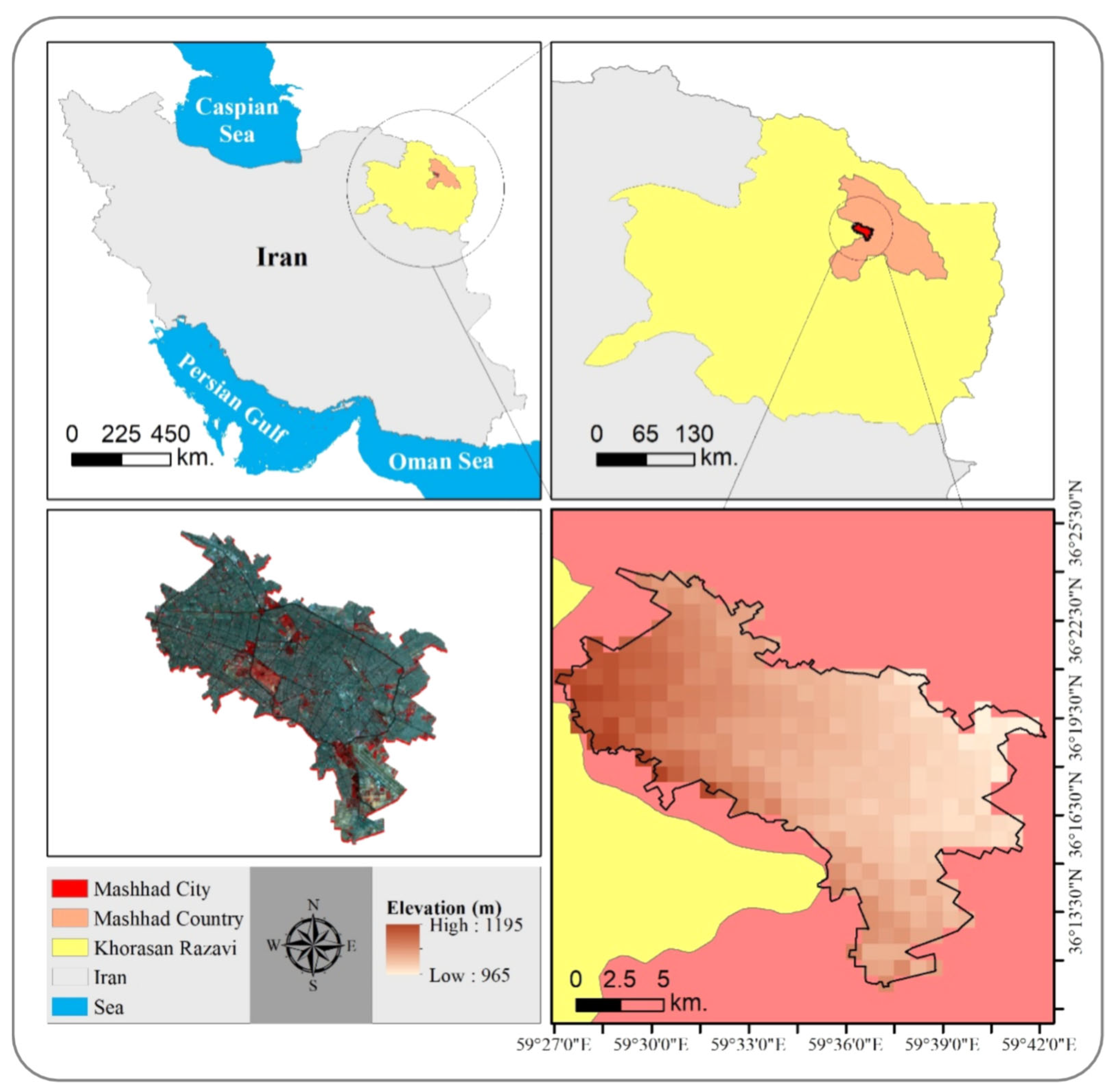
Some cities grow rapidly, irregularly, and without a multiannual development plan or control, which frequently causes environmental and dangerous socioeconomic impacts on individual wellbeing [68], urban ecology [20], urban warming [69], agricultural lands [70], hydrological parameters, and surface microclimate [50,71,72]. Mashhad in Iran is an example of such a metropolitan city, which has been struggling with environmental and anthropogenic heat emitted in the last decade, resulting from considerable LU/LC changes associated with the rapid growth of the population [73]. The purpose of this study is to (i) present the LU/LC changes occurring in Mashhad city in the last three decades, (ii) quantitatively assess the main factors impacting the increase in the LST, (iii) using landscape metrics, investigate the interaction between urban LU/LC and LST trends, and (iv) predict whether the city is going to be warmer or cooler using remote sensing data and statistical methods. Results of the study can provide very useful information to help manage and plan the expansion of residential land fostering environmental sustainability or the share of vegetation in urban areas resulting in the mitigation of negative effects of the UHI.

2. Materials

2.1. Study Area

Mashhad city, the capital of the Mashhad County, is located in the center of Khorasan Razavi province in northeastern Iran, between 36°11′ N and 36°24′ N, and between 59°27′ E and 59°42′ E (Figure 1). The city of Mashhad has an area of 351 km², being the second-largest city in Iran. The average height of the city, extracted from the digital elevation map, is about 1080 m, with a maximum height equal to 1150 m and a minimum of 950 m. Mashhad city lies in an area that can be characterized as a cold, dry, and semi-arid climate (steppe climate, Köppen BSk). In Mashhad, summers are hot, arid, and clear, while the winters are very cold, dry, and partly cloudy. The mean annual rainfall is about 250 mm, and the average annual temperature is 14.3 °C [74]. The closest towns are Ghoochan in the north, Torbat-e Heydarieh in the south, Sabzevar in the west, and Sarakhs in the east. According to statistics published by the Iran National Statistics Portal “www.amar.org.ir” (accessed on 30 July 2020), in the last three decades, Mashhad experienced rapid population growth. According to the latest census published by the Statistical Center of Iran (2016), its population is now equal to 3,372,660.

2.2. Data Collection

To obtain the LU/LC and LST maps of the metropolitan city of Mashhad, satellite images from Landsat downloaded from the United States Geological Survey (USGS) portal [75] were used. To capture changes in the LU/LC and LST, the images were collected at four points in time differing by about a decade. The data came from Landsat 5 Thematic Mapper (TM) (images for 1990 and 2011), Landsat 7 Enhanced Thematic Mapper Plus (ETM+) (image for 2000), and Landsat 8 Operational Land Imager/Thermal Infrared Sensor (OLI/TRIS) (image for 2019). More detailed information regarding the date of image acquisition is provided in

Table 1. The information about the Landsat datasets used to obtain Mashhad LU/LC and LST maps.

Sensor	Scene ID	AQ. Date	AQ. Time (GMT)
Landsat-5 TM	LT05_L1TP_159035_19900930_20171207_01_T1	30 September 1990	05:56:51
Landsat-7 ETM+	LE07_L1TP_159035_20000917_20170210_01_T1	17 September 2000	06:27:44
Landsat-5 TM	LT05_L1TP_159035_20110807_20161009_01_T1	7 August 2011	06:26:06
Landsat-8 OLI/TIRS	LC08_L1TP_159035_20190914_20190917_01_T1	14 September 2019	07:07:15

. The LST maps were obtained using Landsat thermal bands (TM and ETM+ 6th band, as well as Landsat 8 10th band).

3. Methods

3.1. Flowchart of the Data Processing

The flowchart of the data processing is presented in Figure 2. After the data were collected from Landsat 5, 7, and 8 (TM, ETM+, OLI, and TIRS), and after radiometric and atmospheric corrections were made using ENVI software, the maximum likelihood classification and single-change methods were used to obtain LU/LC and land surface temperature maps, respectively, for Mashhad City, Iran. Obtained LU/LC and LST maps were designed and analyzed in the ArcMap environment and correlated with each other to assess their relationship. To study the changes in those quantities that will most probably occur over the next decade (around 2030), the forecast of LU/LC and LST maps was performed using Markov and Ca-Markov models in IDRISI Selva. To ensure that the forecast for 2030 is acceptable, the model was validated by comparing the forecast of the LU/LC and LST maps made for 2011 and 2019 to the actual maps for these years. The developed model included the impact of the population as one of the factors influencing the changes in LU/LC and LST maps. The prediction of population change over the next decade was performed by incorporating demographic data for the study period (Figure 2).

3.2. Methodology

3.2.1. Calculation of Population Growth Rate

Historical Population Growth Rates

To calculate the influence of the changes in population on LU/LC changes in Mashhad, the population statistics for the closest years available in the National Statistical Center of Iran were obtained (

Table 2. Population of Mashhad city (National Statistical Center of Iran, 2020).

Year	1986	1996	2006	2011	2016
Population	2,022,966	2,247,996	2,868,350	3,069,941	3,372,660

), which allowed us to determine the annual growth rates for the each of the studied periods.

The annual growth rates were calculated as

$$r=\left(\sqrt[n]{\frac{P_t}{P_0}}-1\right)·100\%,$$

(1)

where r is the population annual growth rate (as a percentage), n is the length of the period (in years), and P₀ is the population at the beginning while P_t is the population at the end of the period. The annual growth rate for 1990 was calculated from the population changes occurring between 1986 and 1996, for 2000 from the data for 1996 and 2006, and for 2011 from the data for 2000 and 2011.

Prediction of Population

Calculation of the population annual growth rates allowed for the implementation of a population forecasting model [76],

$$P_t=P_0\times {\left(1+r\right)}^n,$$

(2)

which was used to predict the Mashhad population for 2019 and 2030.

3.2.2. LU/LC Classification

The maximum likelihood supervised classifier was used to distinguish classes on LU/LC maps. It was decided that three distinct classes would be used, namely, built-up land (BUL), vegetated land (VL), and bare land (BL) [77], which were revealed in previous LULC and LST analyses [78,79,80] as the main and most effective classes to study LULC in relation to LST. The maximum likelihood supervised classifier was selected because it was previously evaluated to have good accuracy [73].

Maximum Likelihood Method

The maximum likelihood estimation is a method of evaluation of the parameters of the Gaussian probability density function (PDF). It works in such a way that the observed data are given by the chosen statistical model as having the highest probability. The essential diacritic function for each LU/LC class can be described as follows [81]:

$$\begin{gathered} g_i\left(X\right)=p\left(W|w_i\right)p\left(w_i\right) \\ =\frac{p\left({\omega }_i\right)}{{\left(2\pi \right)}^{n/2}{\left|{\Sigma }_i\right|}^{1/2}}\times e^{-\left(\frac{1}{2}\right){\left(X-U_i\right)}^T{\Sigma }_i^{-1}\left(X-U_i\right)}, \end{gathered}$$

(3)

where n is the number of bands, X is the data vector, U_i is the mean vector of the i-th class, and ${\Sigma }_i$is the covariance matrix of class I, defined as follows:

$$X=\left[\begin{array}{c}{x}_i\\ x_i\\ \begin{array}{c}⋮\\ x_n\end{array}\end{array}\right]U_i=\left[\begin{array}{c}{\mu }_{i1}\\ {\mu }_{i2}\\ \begin{array}{c}⋮\\ {\mu }_{in}\end{array}\end{array}\right]{\Sigma }_i=\left[\begin{array}{c}\begin{array}{ccc}{\sigma }_{i11}& {\sigma }_{i12}& \begin{array}{cc}\cdots & {\sigma }_{i1n}\end{array}\end{array}\\ \begin{array}{ccc}{\sigma }_{i21}& {\sigma }_{i22}& \begin{array}{cc}\cdots & {\sigma }_{i2n}\end{array}\end{array}\\ \begin{array}{ccc}⋮ & ⋮ & \begin{array}{cc}\ddots & ⋮\end{array}\end{array}\\ \begin{array}{ccc}{\sigma }_{in1}& {\sigma }_{in2}& \begin{array}{cc}\cdots & {\sigma }_{inn}\end{array}\end{array}\end{array}\right].$$

(4)

The unbiased estimators approximate the values in the mean vector U_i and the covariance matrix ${\Sigma }_i$, from the results of the training:

$${\mu }_{ij}=\frac{1}{P}{{\displaystyle \sum }}_{l=1}^{P_i}{x}_{jl} j=1,2,\dots ,n,$$

(5)

$${\sigma }_{ijk}=\frac{1}{P}{{\displaystyle \sum }}_{l=1}^{P_i}\left(x_{jl}-{\mu }_{ij}\right)\left(x_{kl}-u_{ik}\right) j=1,2,\dots ,n; k=1,2,\dots ,n,$$

(6)

where P_i represents the number of training patterns in the i-th class.

Equation (1) can be reduced by taking the natural logarithm and removing the constant $\pi$ term:

$$g_i\left(\mathrm{X}\right)=lo{g}_{e}p\left({\omega }_i\right)-\frac{1}{2}lo{g}_e\left|{\mathsf{\Sigma }}_i\right|-\frac{1}{2}{\left(X-U_i\right)}^T.{{\displaystyle \sum }}_i^{-1}\left(X-U_i\right).$$

(7)

The equation can be further reduced if it is assumed that the probabilities of the past realizations in the first term are equal. Furthermore, the second term has a constant value for each class, which results in only the third term needing to be calculated for each pixel during classification. The class representative for each pixel is assigned by calculating the diacritic $g_i\left(\mathrm{X}\right)$ distinctly for each class, and then by choosing the one having the highest value.

LU/LC Classification Accuracy Assessment

To determine the classification accuracy for each LU/LC class, a stratified random sampling approach was used. A total of 1000 pixels were chosen randomly from Landsat datasets for each class for all four different points in time [60]. To evaluate the precision of classification, quantities such as the user, producer, and overall accuracy, as well as the Kappa coefficient, were determined [82,83]. The Kappa test is a nonparametric measure used to determine how well user-assigned and predefined values correspond to each other [84]. The Kappa coefficient is usually used as an index of the quality of measurement for binary characteristics. The value of the Kappa coefficient varies in the range from −1.0 to 1.0, with 1.0 interpreted as the perfect agreement of the data (user-assigned and predefined values match each other), 0.0 interpreted as an agreement no better than that expected by chance, and negative values interpreted as an agreement worse than that expected by chance. The Kappa coefficient is determined by the true prevalence of the characters in the sampled population, as well as their susceptibility and specificity for each of the two classifications [85].

3.2.3. Calculation of LST

LST was calculated from the brightness temperature using emissivity correction [60,82,86]:

$$\mathrm{LST}=\left[\frac{\tau }{1+w\left(\frac{\tau }{p}\right)\ln \left(e\right)}\right],$$

(8)

where $\tau$ is the at-sensor brightness temperature, $w$ is the wavelength of emitted radiance (11.5 µm for TM and ETM+ 6th band, and 10.8 µm Landsat 8 TIRS 10th band), and $p=h\times c/s \left(1.438\times {10}^{-2} \mathrm{m}·\mathrm{K}\right)$, with $h$ being the Plank’s constant ($6.626\times {10}^{-34} \mathrm{J}·\mathrm{s}$), $s$ being the Boltzmann Constant ($1.38\times {10}^{-23} \mathrm{J}/\mathrm{K}$), $c$ being the velocity of light ($2.988\times {10}^8 \mathrm{m}/\mathrm{s}$), and $e$ being the land surface emissivity.

The temperature value at the sensor (brightness) was extracted as follows [60,82,86]:

$$\tau =\left[\frac{K_2}{\ln \left(\frac{K_1}{L_{\phi }}+1\right)}\right],$$

(9)

where $K_1$ and $K_2$ are the thermal conversion constants taken from Thematic Mapper (TM) and Enhanced Thematic Mapper+ (ETM+) metadata of the 6th band, and from Landsat 8 Thermal Infrared Sensor (TIRS) metadata of the 10th band (

Table 3. Landsat thermal band conversion constants.

Sensor	Band	K1 [W/(m2·sr·µm)]	K2 [K]
TM	6	607.76	1260.56
ETM+	6	666.09	1282.71
TIRS	10	774.8	1321.0

).

To calculate at-sensor brightness temperature$\tau$ from the thermal bands (TM and ETM+ 6th band, Landsat 8 10th band), raw data were transformed into spectral radiance values as follows [87]:

$$L_{\phi }=M_L\times Q_{Cal}+A_L,$$

(10)

where $L_{\phi }$ is top of atmosphere (TOA) spectral radiance [W/(m²·sr·µm)], $M_L$ is a multiplicative rescaling factor dependent on the metadata for a particular band, $Q_{Cal}$ is the quantized and calibrated standard product’s pixel values (digital number), and $A_L$ is the additive rescaling factor dependent on the metadata for a particular band.

The land surface emissivity $e$ was calculated as follows [60,82,86]:

$$e=n P_v+m,$$

(11)

where $n$ = 0.004 [4] and $m$ = 0.986 [4], and $P_v$ denotes the vegetation proportion, also referred to as fractional vegetation cover.

The vegetation proportion ($P_v$) was calculated as follows [60,82,86]:

$$P_v={\left[\frac{NDVI-NDV{I}_{min}}{NDV{I}_{max}-NDV{I}_{min}}\right]}^2,$$

(12)

where NDVI is the normalized difference vegetation index, and $NDV{I}_{min}$ and $NDV{I}_{max}$ are the minimum and maximum values of the NDVI.

3.2.4. Calculation of NDVI

The NDVI is one of the most important metrics used for the determination of the urban climate [64]. The NDVI value varies from −1 to +1, with high positive values indicating trees, small positive values indicating built-up or bare soils, and negative values indicating water bodies [65]. It delivers information on the abundance, phenology, and wellbeing of vegetation [88]. To measure the NDVI, the reflectance values from red (R) and near-infrared (NIR) bands are used [86,89]:

$$NDVI=\frac{NIR-R}{NIR+R},$$

(13)

where NIR band corresponds to Band 4 in Landsat TM and ETM+ (0.76–0.90 μm) and Band 5 in Landsat 8 OLI (0.85–0.88 μm), while the red (R) band is represented by Band 3 in Landsat TM and ETM+ (0.63–0.69 m) and Band 4 in Landsat 8 OLI (0.64–0.67 m).

Before calculating the NDVI, the reflectance values from the red (R) and near-infrared (NIR) bands were derived as follows [87]:

$${\rho }^{\phi }=M_{\rho }{Q}_{Cal}+A_Q,$$

(14)

where ${\rho }^{\phi }$ is the TOA reflectance without solar angle correction, $M_{\rho }$ is the multiplicative rescaling component depending on the metadata for a given band, $Q_{Cal}$ is the quantized and calibrated standard product’s pixel values (digital number), and $A_Q$ is an additive rescaling component dependent on a metadata band.

3.2.5. LU/LC and LST Prediction

Markov Model for Forecasting of LU/LC and LST Changes

The Markov model is the most commonly used technique for simulating LU/LC changes [90]. In the Markov approach, the future state of a system is predicted on the basis of the knowledge of the states preceding the predicted one. To predict changes in LU/LC for the future period [90], a transition matrix with changes in LU/LC over past periods is developed [91]. The Markov model provides a simple methodology for analyzing and studying complex dynamical systems [90,92,93,94,95]. Several studies have acknowledged the accuracy of the Markov approach [90,95,96]. In the paper, the Markov model was also used to predict the LST changes for Mashhad in 2030.

Markov Model Accuracy Assessment

To assess the accuracy of the developed Markov models for LU/LC and LST prediction, the LU/LC and LST were predicted for 2011 and 2019 and compared with the actual maps derived from the satellite images. To ensure the model’s suitability, the findings were compared to real values using the $\chi$² test [90]:

$$\chi 2=\frac{\sum {\left(O-E\right)}^2}{E},$$

(15)

where E is the map coming from the prediction, and O is the map derived from the satellite image.

4. Results

4.1. Population Changes

In Figure 3, the changes in the population of Mashhad city and corresponding growth rates are presented. The biggest change in the Mashhad population occurred between 1996 and 2006 (by about 600,000 citizens), which was accompanied by the largest value of the annual population growth rate (2.46%). At the same time, a positive change in the annual population growth rate between 1990 and 2000 by 1.4% (from 1.06 to 2.46%) was the largest in the study period. After 2000, the annual population growth rate decreased to 1.63% (by 0.83%) in 2011, and was forecasted to steadily decrease to 0.97% in 2019 (by 0.66%) and 0.62% (by 0.34%) in 2030, but remain positive. The forecast of the Mashhad population showed that, in the period 1986–2030, it would almost double, from ~2 million in 1986 to more than ~3.7 million citizens in 2030.

4.2. LU/LC Classification

4.2.1. Spatiotemporal Pattern of LU/LC

In the study, four points in time separated by approximately a decade (1990, 2000, 2011, and 2019) were used to visualize the spatial dynamics of the LU/LC. In Figure 4, the maps of the LU/LC classification of Mashhad are shown for mentioned years, while, in Figure 5, the area and the share of the area occupied by each of the analyzed LU/LC classes are presented for the same years. Over 30 years, the built-up land (BUL) had an uptrend of about 30 km² per decade, and its area changed from 195 km² in 1990 to 284 km² in 2019. Vegetated land (VL) decreased from 60 km² in 1990 to 44 km² in 2000, while, in the period from 2000 to 2011, its area almost did not change (decreased by less than 1 km²). The downtrend appeared again between 2011 and 2019, and the VL area had decreased by 7 km² to 36 km². BL had a steady downward trend, with the BL area declining from 96 km² in 1990 to 32 km² in 2019. In almost all periods, the share of BL was higher than that of VL. The more severe decline in VL area in the period 1990–2000 than for the other periods led to the highest difference between the share of VL and BL (12%) in 2000. However, the development of Mashhad city in the period 2000–2019 consisting of building mostly on bare land, while replacing the vegetated areas with built-up land in rare cases, only led to a narrowing of the difference between BL and VL. In 2019, the share of BL was even lower than that of VL (Figure 5), while BUL had the highest share of the area in the whole studied period (1990–2019), reaching over 80%.

4.2.2. LU/LC Classification Accuracy Assessment

LU/LC classification accuracy was performed separately for the four selected points in time (1990, 2000, 2011, and 2019). In

Table 4. Accuracy of Mashhad city LU/LC classification for the period of 1990–2019 for built-Up land (BUL), vegetation land (VL), and bare land (BL) classes.

		Year
	LU/LC Class	1990	2000	2011	2019
User accuracy	BUL	95.1	96.7	90.4	99.5
	VL	83.3	82.1	97.3	95.9
	BL	99.3	99.2	99.7	99.2
Producer accuracy	BUL	97.4	97.8	98.6	99.7
	VL	99.4	98.8	99.3	99.9
	BL	97.3	97.4	97.1	99.4
Overall accuracy		97.4	99.5	97.5	97.6
Kappa coefficient		0.93	0.99	0.94	0.95

, the accuracy assessment of Mashhad city LU/LC classification for these years is presented. The user and producer accuracies were larger than 82% in all LU/LC classes in all years, while achieving values greater than 95% in most cases. An overall accuracy higher than 97% and a Kappa coefficient higher than 0.93 were obtained in all years (Table 4).

The obtained results strongly suggest that the maximum likelihood model developed for LU/LC classification in Mashhad city had very high accuracy and could be successfully used for this purpose. Obtained maps passed the minimum accuracy requirements to be used for the subsequent post-classification forecasting operations. To predict the Mashhad city LU/LC, the probability of transition between classes, which determines the likelihood that, in the future, a specific LU/LC class will be replaced by another class, was calculated. In

Table 5. LU/LC transition matrix between 2011 and 2019 (as a percentage) for built-Up land (BUL), vegetation land (VL), and bare land (BL) classes.

2011	2019
	BUL	VL	BL
BUL	13.6	0.1	1.4
VL	0.08	0.08	0.1
BL	1.1	0.008	0.05

, the transition matrix for each LU/LC is presented.

4.3. Spatiotemporal Pattern of LST

In Figure 6,the spatial patterns of the LST for the city of Mashhad during the selected timepoints from a period of 30 years (1990–2019) are presented, while, in Figure 7, the mean value of the LST for Mashhad city for the same years are shown. In the year 2000, the highest increase in LST was observed, with an average LST of 34.5 °C (change by more than 5 °C from 29.2 °C in the period 1990–2000). The upward trend was then reversed with a steep slope from 34.5 °C in 2000 to 30.6 °C in 2011 and almost no change in the mean LST in the period 2011–2019 (from 30.6 °C to 30.5 °C). The highest mean LST in 2000 was probably connected to the highest growth in the population of the Mashhad city and the highest population annual growth rate in the corresponding period (1996–2006). This led to the uncontrolled development of the city, during which a most severe decrease occurred in VL (by 16 km², representing 4.8% of the total city area) in the preceding period (1990–2000), along with an increase in the share of BUL by 7.7% of the total area and a less noticeable decrease in BL (by 2.9%), which led to the highest difference between the shares of VL and BL (12%), as shown in Figure 5. By comparing the spatial patterns shown in Figure 4 and Figure 6, it can be deduced that, in the study area, the highest values of LST were observed for BL, whereas the lowest were observed for VL. Therefore, the high reduction in VL in the period 1990–2000 led to a higher LST in 2000. In 2011, despite a 9.6% increase in BUL, a 9.5% decrease in BL, and a very minor change in VL (0.1%) compared to the previous period (2000), a decrease in the mean LST could be observed. Similarly for 2019, despite an 8% increase in BUL, a 2% decrease in VL, and a 5.9% decrease in BL, compared to the previous period (2011), the mean LST almost did not change and was equal to 30.5 °C (Figure 7). The observed reduction in LST was probably connected to the more controlled and planned development of the Mashhad city in the period 2000–2019, consisting of building mostly on bare land, while replacing the vegetated areas with built-up land in rare cases only, which resulted in the VL, unlike previous years, occupying a larger area than BL2019. A high reduction in the hottest LU/LC type (BL), along with an almost unchanged or minor decrease in the share of VL, probably caused the effect of LST stabilization at the 30.5 °C level.

4.4. Prediction of LU/LC and LST

4.4.1. Assessment of the Accuracy of the Markov Model for LU/LC and LST Prediction

To validate the developed model and ensure its suitability, the simulated LU/LC and LST should be firstly compared to the real data. To do so, the data obtained from the satellite images for 2011 and 2019 were compared to the Markov model prediction of the LU/LC and LST for 2011 and 2019. In the paper, only the results of the LU/LC comparison obtained for 2011 (Figure 8 and

Table 6. Validation statistics of Markov model LU/LC prediction for 2011 for built-up land (BUL), vegetation land (VL), and bare land (BL) classes.

LU/LC Class	Simulated Value (E) 2011 (km2)	Actual Value (O) 2011 (km2)	$\mathit{O}-\mathit{E}$	${\left(\mathit{O}-\mathit{E}\right)}^2$	${\left(\mathit{O}-\mathit{E}\right)}^2/\mathit{E}$
BUL	280.41	283.43	−3.02	9.13	0.03
VL	38.65	36.09	2.56	6.56	0.17
BL	31.94	31.48	0.46	0.21	0.01

Note: $\chi 2=\frac{\sum {\left(O-E\right)}^2}{E}$ = 0.106; degree of freedom = 2; $\chi 2$ _0.05 (2) = 5.99 [90].

) and LST comparison for 2019 (Figure 9 and

Table 7. Validation statistics of Markov model LST map prediction for 2019.

LST Class	Simulated Value (E) 2019 (km2)	Actual Value (O) 2019 (km2)	$\mathit{O}-\mathit{E}$	${\left(\mathit{O}-\mathit{E}\right)}^2$	${\left(\mathit{O}-\mathit{E}\right)}^2/\mathit{E}$
26–32	47.41	44.95	2.46	6.06	0.13
32–34	127.86	127.42	0.45	0.20	0.00
34–36	95.33	95.43	−0.09	0.01	0.00
36–38	51.95	53.37	−1.42	2.01	0.04
38–44	28.43	29.83	−1.40	1.96	0.07

Note: $\chi 2=\frac{\sum {\left(O-E\right)}^2}{E}$ = 0.237; degree of freedom = 4; $\chi 2$ _0.05 (4) = 9.49 [90].

) are presented. The results were compared to real values using the $\chi$² test [90].

Obtained results (Table 6 and Table 7) indicate that the disparity between simulated and actual values of the LU/LC and LST was negligible. The ${\chi }^2$ test value for the comparison between the simulated and actual Mashhad city LU/LC maps for 2011 was equal to 0.106, whereas that for the comparison between the simulated and actual Mashhad city LST maps for 2019 was equal to 0.237. In conclusion, the developed Markov model was suitable and could be successfully used to predict the LU/LC and LST of Mashhad.

4.4.2. Markov Model Forecast of the Changes in the LU/LC and LST for 2030

Figure 10 shows the forecast of LU/LC and LST maps of Mashhad city for 2030 (panels a and b, respectively), along with the comparison of the changes in LU/LC and LST that occurred compared to 2019 (panels c, d, and e). Regarding LU/LC compared to 2019, the forecast for 2030 indicated further declines in VL (by 25% in relation to the area occupied by VL in 2019) and BL (by 77%) in favor of an increase in BUL (by 12%) (Figure 10e). In 2030, BL was projected to decrease from 32 to 7.5 km² (by 24 km²), VL was projected to decrease from 36 to 27 km² (by 9 km²), and BUL was projected to increase from 284 to 317.5 km² (by 33.5 km²) (Figure 10a,b). The trend of LU/LC changes, together with an effect of population growth suggested by the forecast of Mashhad city population, showed that, in 2030, around 350,000 more citizens will live in Mashhad compared to 2016 (rise from 3,372,660 to 3,716,991 people), which could cause a serious crisis connected with LST rise (Figure 10c,d). As shown in Figure 10d, the area of land having a value of LST <36 °C will significantly decrease compared to 2019. On the other hand, the area of land having LST ≥36 °C will significantly increase. In 2019, the largest area (153.4 km²) had LST values ranging from 32 to 34 °C, whereas, for 2030, it was predicted that the largest area (169.2 km²) will have LST values ranging from 36 °C to 38 °C. Further development of the city and a reduction in VL areas forecasted for 2030 would result in cooler areas no longer fulfilling their cooling function. The VL areas with LST ranging from 26 °C to 32 °C in 2019 were predicted to increase LST to the range of 34–38 °C in 2030. The obtained results show that one should expect not only that the temperature of most of the city will increase in 2030 by about 4 °C, but also that a shift in temperature distribution toward higher values will occur. The mean value of LST for 2030 was predicted to have a value of 36.5 °C.

5. Discussion

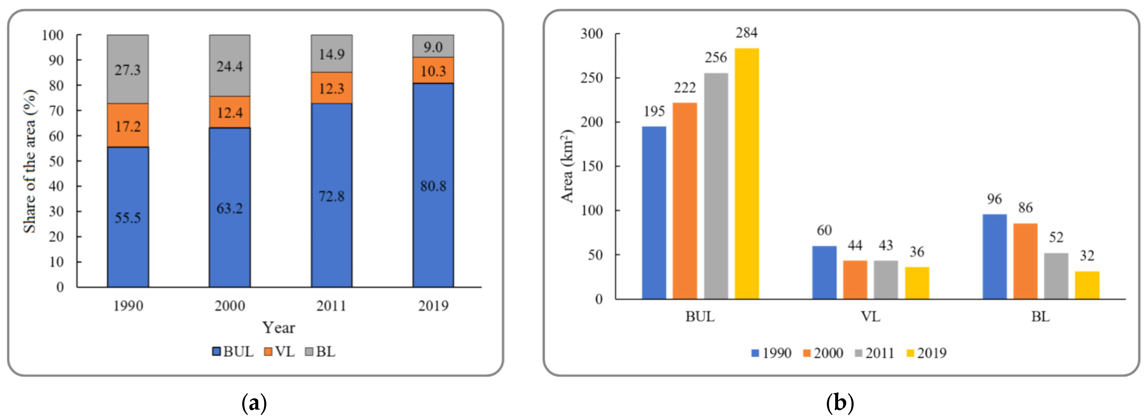
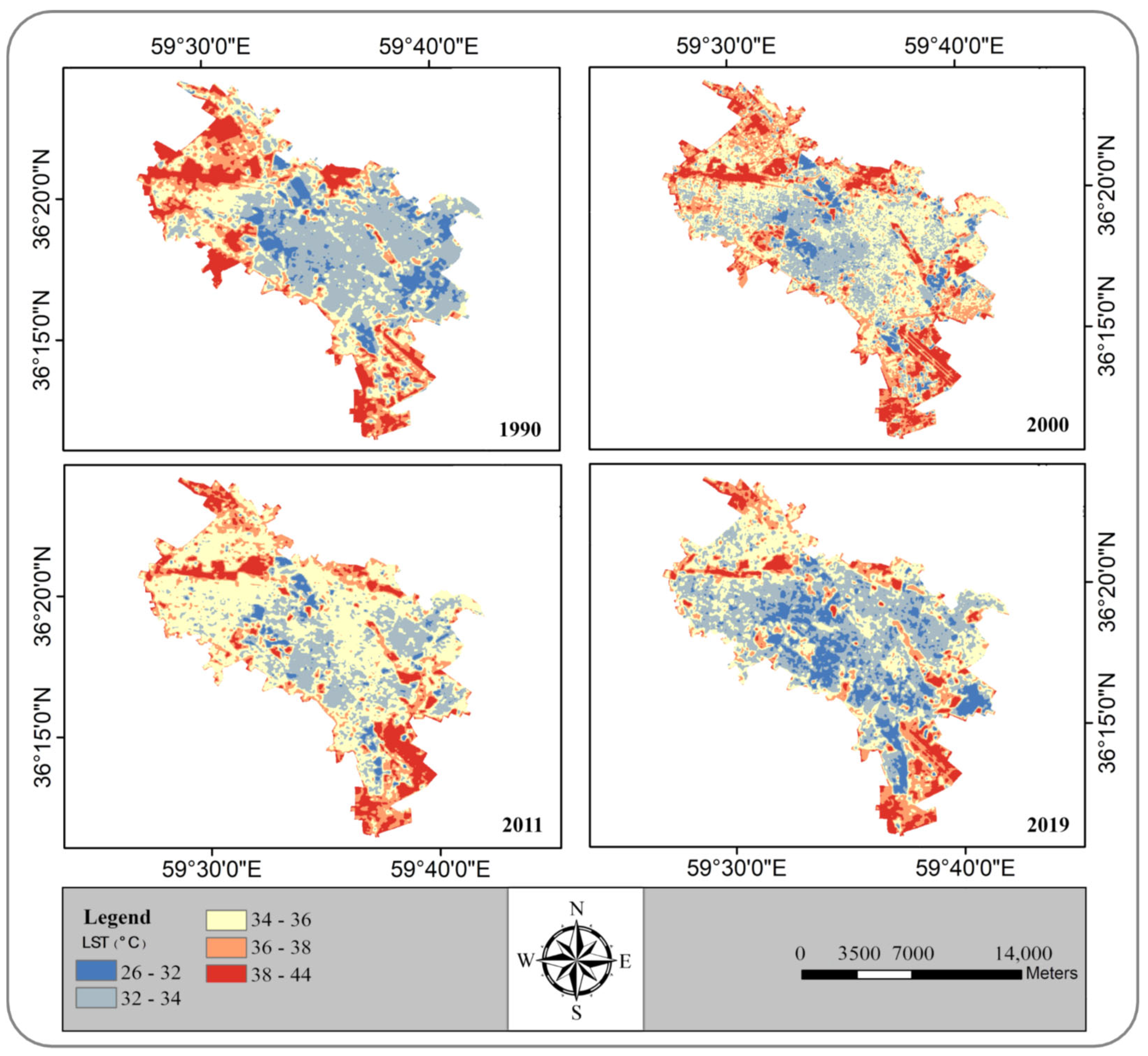
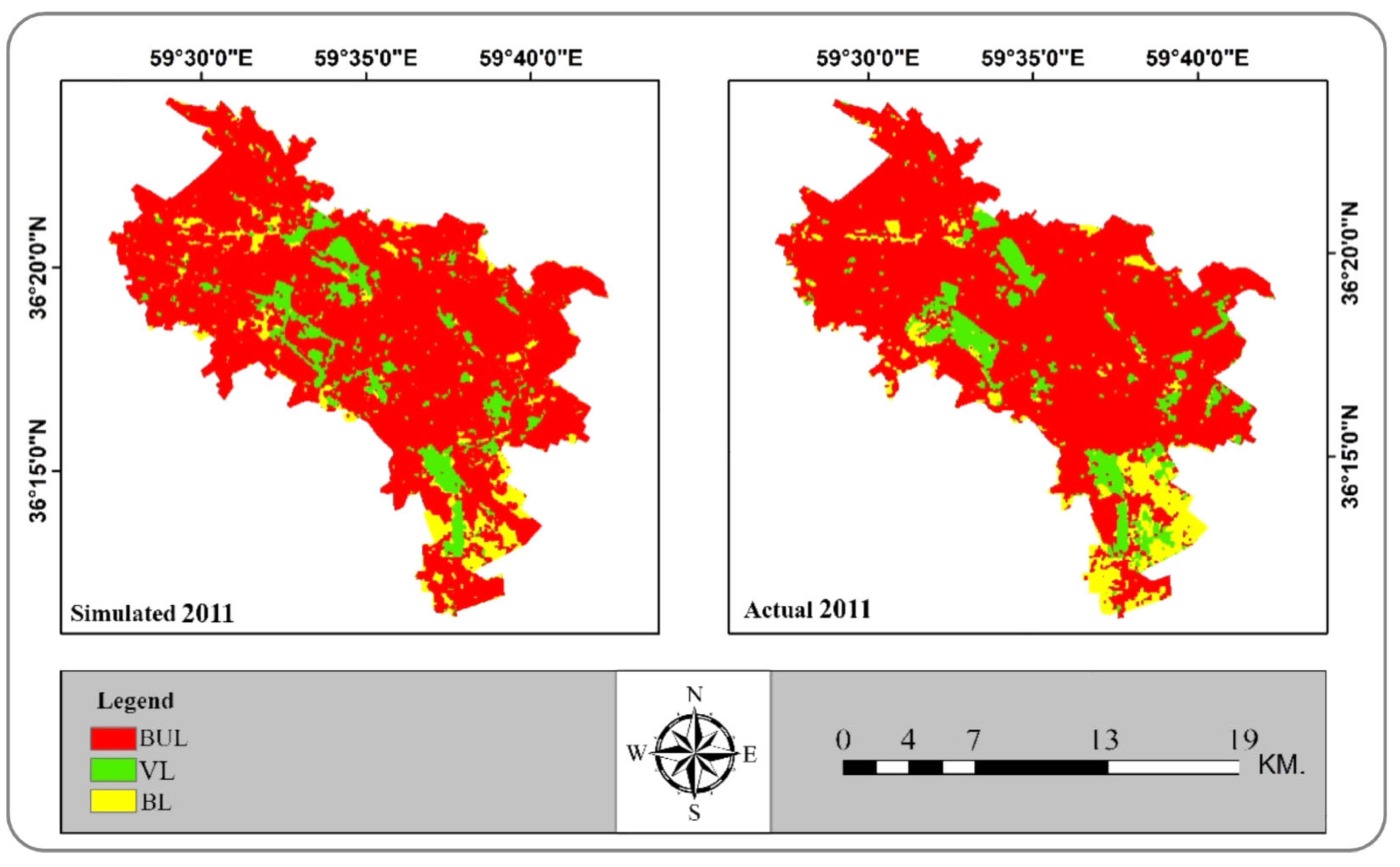
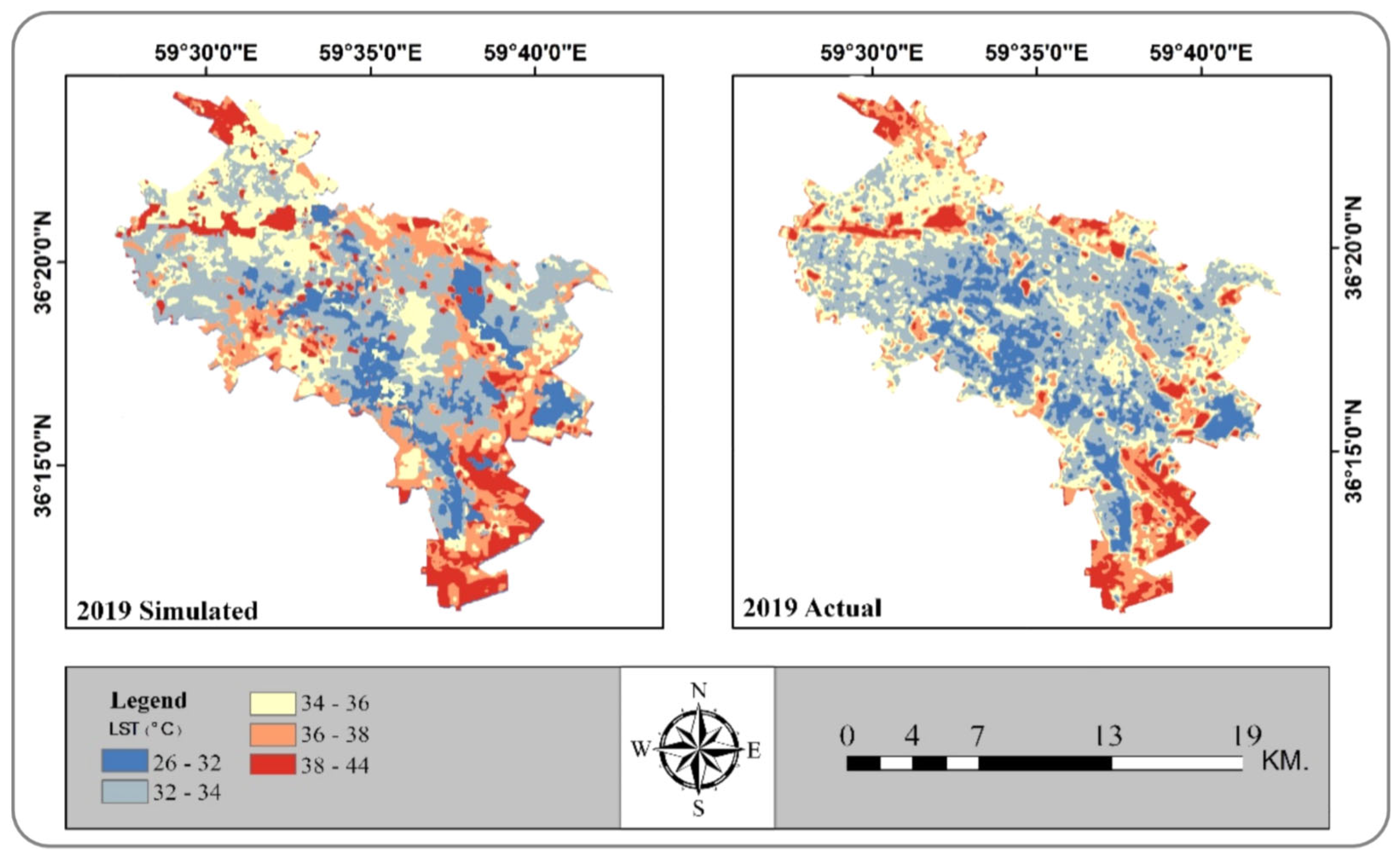
From the results, it seems that, in the period from 1990 to 2019, the impervious surface area (BUL) in Mashhad city expanded from 195 km² (55.5% of the total area of the city) to 284 km² (80.8% of the total area), while areas with vegetation (VL) shrank from 60 km² (17.2% of total area) to 36 km² (10.3% of total area). This increase in class BUL and the decrease in class VL in their favor can be justified by the population growth in the statistical period (discussed later). The average LST increased slightly, from 29.2 °C to 30.5 °C, in the period from 1990 to 2019, by reducing VL classes and replacing them with BUL. VL had a relatively lower mean LST than the other LU/LC classes, equal to 26.6 °C in 1990, 32.6 °C in 2000, 33.3 °C in 2011, and 28.2 °C in 2019, indicating a class VL cooling effect, possibly due to factors such as shade, water, and transpiration. On the other hand, the highest mean LST was observed for bare land (BL), equal to 33.4 °C in 1990, 39.2 °C in 2000, 39.2 °C in 2011, and 33.2 °C in 2019, potentially due to the lack of human cooling activities (such as tree planting and irrigation or the use of cooling equipment), as well as the lack of vegetation and the absorption of direct energy by the bare soil.

Between 1990 and 2000, a 7.7% increase in BUL (to 222 km²), a 4.8% decrease in VL (to 44 km²), and a nearly 3% decrease in BL (to 86 km²) probably resulted in the highest mean LST being observed in 2000 across the whole study period (34.5 °C). Furthermore, a decrease in the share of BLs to 14.9% of the total city area (52 km²) in a subsequent period (2000 to 2011), a change in VL < 1% (to 43 km²), and a decrease by 0.83% in population annual growth rate caused the mean value of the LST to decrease by about 4 °C. The trend of changes in Mashhad city LU/LC persisted in the next period (2011–2019). BUL increased by 8% (to 284 km²), while VL and BL decreased by 2% (to 36 km²) and 5.9% (to 32 km²), respectively. The comparison of the Mashhad LU/LC and LST maps for the studied period (1990–2019) indicates that the share of the BL and BUL area had a significant effect on LST, as the increase in the share of these two classes, along with a simultaneous decrease in VL, increased the mean LST of the city. The obtained results indicate that the effect of changes in BL on the LST was more significant than for changes in BUL, which may be connected to the fact that, in BUL, a small share of the plants and water cover may be present. In the period between 1990 and 2000, the highest value of the population annual growth rate was obtained for the whole study period.

The fluctuations in population annual growth rate are consistent with the fluctuations in LST (R = 0.94, p-value = 0.01), i.e., a period with an increase in population annual growth rate was also the period with an increase in mean LST, while the decrease in population annual growth rate coincided with a decrease in mean LST. This is because a positive population annual growth rate is somehow connected to and forces changes in LU/LC (a higher population annual growth rate usually implies a greater increase in BUL and reductions in BL and VL) The negative relationship between the cooling influence of green areas and LST [44,45,46,47,48,49] and the high thermal energy storage capacity of urban areas [97] shown in previous studies can support this claim. This correlation is probably due to the reduction in VL areas, which are having a cooling effect on the LST in the cities and build-up on BL (due to the effect of their ventilation compared to the BUL). Furthermore, the expansion of UIL and the expansion of VL, both of which are areas prone to high thermal absorption, result in a rise in the thermal absorption associated with heat islands in cities [98,99,100]. The above findings are in line with the findings of Alavipanah et al. [74]. Other studies assessing the impact of the spatial pattern of the urban LU/LC on LST in Mashhad, e.g., Soltanifard and Aliabadi (2019), claimed that Mashhad’s integrated urban cover had a cooler temperature than other forms of cover [101].

The LU/LU forecast for 2030 in this study, which has very rarely been performed in studies dealing with this subject [67,101,102], showed that the area of BUL increased by 12% (to 317.5 km²), while VL and BL decreased by 25% (to 27 km²) and 77% (to 7.5 km²), respectively, compared to 2019. This increasing trend of class BUL along with the decrease in class VL and BL is justifiable according to the trend observed in the statistical period and the growth of the urban population in Mashhad. Noteworthily, the rate at which metropolitan regions are growing can surpass all expectations. such that it may continue outside the city limits, as examined in specialized studies [103,104]. However, the classification made for 2019 LULC indicated that BUL areas consisted of 80% of all areas, with there still being room for the expansion of BUL areas; furthermore, due to the technical constraints of the used model and the fact that the present study’s forecasts are based on earlier land use/land cover maps, as well as the specificity of model development, this case cannot be considered for areas outside of the borders. Although these results of forecasting are in line with the increase in built-up (BUL) and the decrease in vegetation area (VL) in Rahnama’s (2020) study on LU/LC forecasting in Mashhad for 2030, in terms of increasing bare lands (BL), their research forecast of a 5.5% increase is not compatible [105]. The population forecast for 2030 also showed an increase of about 240,000 citizens compared to 2019, and of about 350,000 citizens compared to the year with the last census available, 2016. A significant increase in the share of BUL for the forecasted period (2019–2030) compared to the previous period (2011–2019), with a simultaneous reduction in VL area by 25%, can be a warning signal to urban planners for the coming years. Raigani et al. (2018) predicted the changes in LU/LC in Mashhad City for the period from 2014 to 2030 and indicated that that BUL is expected to increase by about 10.6%, while the areas of VL and agricultural lands would decrease by 19.3% and 20.5%, respectively. This result is in line with the results presented herein [102]. They also predicted that, in Mashhad in the period 2014–2030, a 3% increase in BL is expected, which is completely different from the 77% decrease in barren land forecasted by our model.

6. Conclusions

In this study, the relationship between the LST and LU/LC for Mashhad city in the period 1990–2030 was evaluated. Using remote sensing data and spatial simulation techniques, the spatiotemporal changes in specific LU/LC classes (BUL, VL, and BL) in the period from 1990 to 2030 were assessed. The obtained results also present how the spatial pattern of Mashhad LST fluctuated over the studied period. The results suggest that the BL areas had a greater impact on the mean LST than other land uses. On the other hand, the lowest values of LST were observed for the VL. The increase in BUL area, along with a reduction in VL area, which plays a major role in the cooling of the city, and a simultaneous reduction in BL area, which provides more ventilation than BUL areas, caused an increase in LST in Mashhad city during the analyzed period of 1990–2019. The fluctuations observed in the Mashhad population annual growth rate are consistent with the fluctuations in mean values of the LST. The forecast of the LST for 2030 indicates that an increase in the mean LST should be expected. Our results suggest that an increase in green areas such as parks, trees, lawns, etc. in the cities can be an effective action leading to a reduction in surface temperature and preventing the creation and expansion of thermal islands in the cities. The conducted research complements and extends the results obtained in the literature [102]. The factor distinguishing our calculations from other studies is the consideration of the population in the assessment of the variability of LST. Secondly, in addition to the prediction of LU/LC only, the LST and population were forecasted in our study. Additionally, the study included the assessment of the effective parameters influencing LST changes and their relationship with LU/LC variations by means of remote sensing, statistical methods, and demographic data, which were rarely applied in other studies on urban analysis. This research advises policymakers and urban planners of Mashhad city to plan carefully in order to prevent the city’s excessive growth, as well as manage urban green spaces with regard to their cooling effect and reintroduce vegetation into the city by building larger park areas that can help release moisture into the atmosphere, planting trees to shade building surfaces and asphalt, and converting rooftops into “green” roofs to deflect radiation from the sun.

References

1. Shayegan, M.; Alimohammadi, A.; Mansourian, A. Multi-objective optimization of land use allocation using NSGA-II algorithm. Iran. Remote Sens. GIS 2013, 10, 163–190. [Google Scholar]
2. Sharifi, L.; Rasuli, A.A.; Hejazi, M.; Roastamzade, H. Land Cover/Use Changes Detection by Object-Oriented Processing Satellite Image Dates (Case Study: Tabriz County). J. Geogr. Plan. 2013, 17, 203–214. [Google Scholar]
3. Omidvar, K.; Narangifard, M.; Abbasi, H. Detection of land use and vegetation changes in Yasuj city using remote sensing. Geogr. Reg. Urban Plan. 2013, 5, 111–126. [Google Scholar]
4. Liu, Z.; Xu, J.; Liu, M.; Yin, Z.; Liu, X.; Yin, L.; Zheng, W. Remote sensing and geostatistics in urban water-resource monitoring: A review. Mar. Freshw. Res. 2023. [Google Scholar] [CrossRef]
5. Zhao, F.; Song, L.; Peng, Z.; Yang, J.; Luan, G.; Chu, C.; Ding, J.; Feng, S.; Jing, Y.; Xie, Z. Night-time light remote sensing mapping: Construction and analysis of ethnic minority development index. Remote Sens. 2021, 13, 2129. [Google Scholar] [CrossRef]
6. Bakhshi Lomer, A.R.; Rezaeian, M.; Rezaei, H.; Lorestani, A.; Mijani, N.; Mahdad, M.; Raeisi, A.; Arsanjani, J.J. Optimizing Emergency Shelter Selection in Earthquakes Using a Risk-Driven Large Group Decision-Making Support System. Sustainability 2023, 15, 4019. [Google Scholar] [CrossRef]
7. Mansourmoghaddam, M.; Ghafarian Malamiri, H.R.; Arabi Aliabad, F.; Fallah Tafti, M.; Haghani, M.; Shojaei, S. The Separation of the Unpaved Roads and Prioritization of Paving These Roads Using UAV Images. Air Soil Water Res. 2022, 15, 11786221221086285. [Google Scholar] [CrossRef]
8. Mansourmoghaddam, M.; Rousta, I.; Ghafarian Malamiri, H. Evaluation of the classification accuracy of NDVI index in the preparation of land cover map. Desert 2022, 27, 329–341. [Google Scholar]
9. Mansourmoghaddam, M.; Rousta, I.; Ghaffarian, H.; Mokhtari, M.H. Evaluating the capability of spatial and spectral fusion in land-cover mapping enhancement. Earth Obs. Geomat. Eng. 2022, 6, 161–174. [Google Scholar]
10. Alberti, M.; Marzluff, J.M. Ecological resilience in urban ecosystems: Linking urban patterns to human and ecological functions. Urban Ecosyst. 2004, 7, 241–265. [Google Scholar] [CrossRef]
11. Gupta, A.; Moniruzzaman, M.; Hande, A.; Rousta, I.; Olafsson, H.; Mondal, K.K. Estimation of particulate matter (PM 2.5, PM 10) concentration and its variation over urban sites in Bangladesh. SN Appl. Sci. 2020, 2, 1–15. [Google Scholar] [CrossRef]
12. Saffarzadeh, M.; Rezaei, H.; Majidi, M.Z. A Pricing Model for Freeway Tolls Based on the Share of Mode Shift, Route Shift, Travel Time Change and Users’ Willingness to Pay (Case study: Tehran_Saveh Freeway). J. Transp. Res. 2022, 19, 359–370. [Google Scholar]
13. He, F.; Mohamadzadeh, N.; Sadeghnejad, M.; Ingram, B.; Ostovari, Y. Fractal Features of Soil Particles as an Index of Land Degradation under Different Land-Use Patterns and Slope-Aspects. Land 2023, 12, 615. [Google Scholar] [CrossRef]
14. Rousta, I.; Sarif, M.O.; Gupta, R.D.; Olafsson, H.; Ranagalage, M.; Murayama, Y.; Zhang, H.; Mushore, T.D. Spatiotemporal analysis of land use/land cover and its effects on surface urban heat island using Landsat data: A case study of Metropolitan City Tehran (1988–2018). Sustainability 2018, 10, 4433. [Google Scholar] [CrossRef]
15. Wang, R.; Derdouri, A.; Murayama, Y. Spatiotemporal simulation of future land use/cover change scenarios in the Tokyo metropolitan area. Sustainability 2018, 10, 2056. [Google Scholar] [CrossRef]
16. Mamdoohi, A.R.; Rezaei, H.; Irannezhad, E.; Saffarzadeh, A.; Abbasi, M. Hour-and Period-based congestion pricing, case of Tehran mode choice. Q. J. Transp. Eng. 2022, 14, 54. [Google Scholar]
17. Mansourmoghaddam, M.; Ghafarian Malamiri, H.R.; Rousta, I.; Olafsson, H.; Zhang, H. Assessment of Palm Jumeirah Island’s Construction Effects on the Surrounding Water Quality and Surface Temperatures during 2001–2020. Water 2022, 14, 634. [Google Scholar] [CrossRef]
18. Ackerman, B. Temporal march of the Chicago heat island. J. Clim. Appl. Meteorol. 1985, 24, 547–554. [Google Scholar] [CrossRef]
19. Kaloustian, N.; Diab, Y. Effects of urbanization on the urban heat island in Beirut. Urban Clim. 2015, 14, 154–165. [Google Scholar] [CrossRef]
20. Grimm, N.B.; Faeth, S.H.; Golubiewski, N.E.; Redman, C.L.; Wu, J.; Bai, X.; Briggs, J.M. Global change and the ecology of cities. Science 2008, 319, 756–760. [Google Scholar] [CrossRef]
21. Coseo, P.; Larsen, L. How factors of land use/land cover, building configuration, and adjacent heat sources and sinks explain Urban Heat Islands in Chicago. Landsc. Urban Plan. 2014, 125, 117–129. [Google Scholar] [CrossRef]
22. Moniruzzaman, M.; Thakur, P.K.; Kumar, P.; Ashraful Alam, M.; Garg, V.; Rousta, I.; Olafsson, H. Decadal Urban Land Use/Land Cover Changes and Its Impact on Surface Runoff Potential for the Dhaka City and Surroundings Using Remote Sensing. Remote Sens. 2021, 13, 83. [Google Scholar] [CrossRef]
23. He, B.-J.; Zhu, J.; Zhao, D.-X.; Gou, Z.-H.; Qi, J.-D.; Wang, J. Co-benefits approach: Opportunities for implementing sponge city and urban heat island mitigation. Land Use Policy 2019, 86, 147–157. [Google Scholar] [CrossRef]
24. He, B.-J. Towards the next generation of green building for urban heat island mitigation: Zero UHI impact building. Sustain. Cities Soc. 2019, 50, 101647. [Google Scholar] [CrossRef]
25. Qiao, Z.; Liu, L.; Qin, Y.; Xu, X.; Wang, B.; Liu, Z. The impact of urban renewal on land surface temperature changes: A case study in the main city of Guangzhou, China. Remote Sens. 2020, 12, 794. [Google Scholar] [CrossRef]
26. Alavipanah, S.K.; Mansourmoghaddam, M.; Gomeh, Z.; Galehban, E.; Hamzeh, S. The reciprocal effect of global warming and climatic change (new perspective): A review. Desert 2022, 27, 291–305. [Google Scholar]
27. Jaber, S.M. Landsat-based vegetation abundance and surface temperature for surface urban heat island studies: The tale of Greater Amman Municipality. Ann. GIS 2018, 24, 195–208. [Google Scholar] [CrossRef]
28. Hewitt, V.; Mackres, E.; Shickman, K. Cool policies for Cool Cities: Best Practices for Mitigating Urban Heat Islands in North American Cities; ACEEE: Washington, DC, USA, 2014. [Google Scholar]
29. Ruijsink, S. Integrating Climate Change into City Development Strategies (CDS): Climate Change and Strategic Planning; UN-HABITAT: Nairobi, Kenya, 2015. [Google Scholar]
30. Amiri, R.; Weng, Q.; Alimohammadi, A.; Alavipanah, S.K. Spatial–temporal dynamics of land surface temperature in relation to fractional vegetation cover and land use/cover in the Tabriz urban area, Iran. Remote Sens. Environ. 2009, 113, 2606–2617. [Google Scholar] [CrossRef]
31. Hong, J.-W.; Hong, J. Changes in the Seoul metropolitan area urban heat environment with residential redevelopment. J. Appl. Meteorol. Climatol. 2016, 55, 1091–1106. [Google Scholar] [CrossRef]
32. Liu, G.; Chen, S.; Gu, J. Urban renewal simulation with spatial, economic and policy dynamics: The rent-gap theory-based model and the case study of Chongqing. Land Use Policy 2019, 86, 238–252. [Google Scholar] [CrossRef]
33. Temme, A.; Sadeghnejad, M.; Sodhi, H.S.; Samia, J. The Search for Path-Dependency Mechanisms Using Physically-Based Soil-Landscape Modelling of Landslides. In Proceedings of the EGU General Assembly 2023, Vienna, Austria, 24–28 April 2023. [Google Scholar]
34. Deakin, M.; Allwinkle, S. Urban regeneration and sustainable communities: The role of networks, innovation, and creativity in building successful partnerships. J. Urban Technol. 2007, 14, 77–91. [Google Scholar] [CrossRef]
35. Fei, H.; Jian-ming, C. The evolution and reconstruction of peri-urban rural habitat in China. Geogr. Res. 2011, 30, 1271–1284. [Google Scholar]
36. Hou, H.; Ding, F.; Li, Q. Remote sensing analysis of changes of urban thermal environment of Fuzhou city in China in the past 20 years. J. Geo-Inf. Sci. 2018, 20, 385–395. [Google Scholar]
37. Peng, C.; Ming, T.; Tao, Y.; Peng, Z. Numerical analysis on the thermal environment of an old city district during urban renewal. Energy Build. 2015, 89, 18–31. [Google Scholar] [CrossRef]
38. Pan, Z.; Wang, G.; Hu, Y.; Cao, B. Characterizing urban redevelopment process by quantifying thermal dynamic and landscape analysis. Habitat Int. 2019, 86, 61–70. [Google Scholar] [CrossRef]
39. Zhang, Y.; Luo, J.; Zhang, Y.; Huang, Y.; Cai, X.; Yang, J.; Mao, D.; Li, J.; Tuo, X.; Zhang, Y. Resolution Enhancement for Large-Scale Real Beam Mapping Based on Adaptive Low-Rank Approximation. IEEE Trans. Geosci. Remote Sens. 2022, 60, 1–21. [Google Scholar] [CrossRef]
40. Piringer, M.; Grimmond, C.S.B.; Joffre, S.M.; Mestayer, P.; Middleton, D.; Rotach, M.; Baklanov, A.; De Ridder, K.; Ferreira, J.; Guilloteau, E. Investigating the surface energy balance in urban areas–recent advances and future needs. Water Air Soil Pollut. Focus 2002, 2, 1–16. [Google Scholar] [CrossRef]
41. Grimmond, C. Progress in measuring and observing the urban atmosphere. Theor. Appl. Climatol. 2006, 84, 3–22. [Google Scholar] [CrossRef]
42. Yang, J.; Fu, L.-Y.; Zhang, Y.; Han, T. Temperature-and pressure-dependent pore microstructures using static and dynamic moduli and their correlation. Rock Mech. Rock Eng. 2022, 55, 4073–4092. [Google Scholar] [CrossRef]
43. Xiao, H.; Weng, Q. The impact of land use and land cover changes on land surface temperature in a karst area of China. J. Environ. Manag. 2007, 85, 245–257. [Google Scholar] [CrossRef]
44. Weng, Q.; Lu, D.; Schubring, J. Estimation of land surface temperature–vegetation abundance relationship for urban heat island studies. Remote Sens. Environ. 2004, 89, 467–483. [Google Scholar] [CrossRef]
45. Islam, S.; Ma, M. Geospatial monitoring of land surface temperature effects on vegetation dynamics in the Southeastern Region of Bangladesh from 2001 to 2016. ISPRS Int. J. Geo-Inf. 2018, 7, 486. [Google Scholar] [CrossRef]
46. Wu, D.; Zhao, X.; Liang, S.; Zhou, T.; Huang, K.; Tang, B.; Zhao, W. Time-lag effects of global vegetation responses to climate change. Glob. Change Biol. 2015, 21, 3520–3531. [Google Scholar] [CrossRef] [PubMed]
47. Guha, S.; Govil, H. An assessment on the relationship between land surface temperature and normalized difference vegetation index. Environ. Dev. Sustain. 2020, 23, 1944–1963. [Google Scholar] [CrossRef]
48. Rousta, I.; Olafsson, H.; Moniruzzaman, M.; Ardö, J.; Zhang, H.; Mushore, T.D.; Shahin, S.; Azim, S. The 2000–2017 drought risk assessment of the western and southwestern basins in Iran. Model. Earth Syst. Environ. 2020, 6, 1201–1221. [Google Scholar] [CrossRef]
49. Jiang, J.; Tian, G. Analysis of the impact of land use/land cover change on land surface temperature with remote sensing. Procedia Environ. Sci. 2010, 2, 571–575. [Google Scholar] [CrossRef]
50. Carlson, T.N.; Arthur, S.T. The impact of land use—Land cover changes due to urbanization on surface microclimate and hydrology: A satellite perspective. Glob. Planet. Change 2000, 25, 49–65. [Google Scholar] [CrossRef]
51. Chen, X.-L.; Zhao, H.-M.; Li, P.-X.; Yin, Z.-Y. Remote sensing image-based analysis of the relationship between urban heat island and land use/cover changes. Remote Sens. Environ. 2006, 104, 133–146. [Google Scholar] [CrossRef]
52. Wang, P.; Yu, P.; Lu, J.; Zhang, Y. The mediation effect of land surface temperature in the relationship between land use-cover change and energy consumption under seasonal variations. J. Clean. Prod. 2022, 340, 130804. [Google Scholar] [CrossRef]
53. EPA. Chapter 1: Urban Heat Island Basics. In Heat Island Compendium; United States Environmental Protection Agency: Washington, DC, USA, 2017. [Google Scholar]
54. Chander, G.; Markham, B.L.; Helder, D.L. Summary of current radiometric calibration coefficients for Landsat MSS, TM, ETM+, and EO-1 ALI sensors. Remote Sens. Environ. 2009, 113, 893–903. [Google Scholar] [CrossRef]
55. Lo, C.; Quattrochi, D.A. Land-use and land-cover change, urban heat island phenomenon, and health implications. Photogramm. Eng. Remote Sens. 2003, 69, 1053–1063. [Google Scholar] [CrossRef]
56. Lin, X.; Zhang, W.; Huang, Y.; Sun, W.; Han, P.; Yu, L.; Sun, F. Empirical estimation of near-surface air temperature in China from MODIS LST data by considering physiographic features. Remote Sens. 2016, 8, 629. [Google Scholar] [CrossRef]
57. Nichol, J.E. High-resolution surface temperature patterns related to urban morphology in a tropical city: A satellite-based study. J. Appl. Meteorol. 1996, 35, 135–146. [Google Scholar] [CrossRef]
58. Mansourmoghaddam, M.; Naghipur, N.; Rousta, I.; Ghaffarian, H.R. Temporal and spatial monitoring and forecasting of suspended dust using google earth engine and remote sensing data (Case Study: Qazvin Province). Desert Manag. 2022, 10, 77–98. [Google Scholar]
59. Borana, S.; Yadav, S. Prediction of land cover changes of Jodhpur city using cellular automata Markov modelling techniques. Int. J. Eng. Sci. 2017, 17, 15402–15406. [Google Scholar]
60. Bokaie, M.; Zarkesh, M.K.; Arasteh, P.D.; Hosseini, A. Assessment of urban heat island based on the relationship between land surface temperature and land use/land cover in Tehran. Sustain. Cities Soc. 2016, 23, 94–104. [Google Scholar] [CrossRef]
61. Mansourmoghaddam, M.; Rousta, I.; Zamani, M.; Mokhtari, M.H.; Karimi Firozjaei, M.; Alavipanah, S.K. Study and prediction of land surface temperature changes of Yazd city: Assessing the proximity and changes of land cover. J. RS GIS Nat. Resour. 2021, 12, 1–27. [Google Scholar]
62. Li, X.; Zhou, Y.; Asrar, G.R.; Imhoff, M.; Li, X. The surface urban heat island response to urban expansion: A panel analysis for the conterminous United States. Sci. Total Environ. 2017, 605, 426–435. [Google Scholar] [CrossRef]
63. Sultana, S.; Satyanarayana, A. Urban heat island intensity during winter over metropolitan cities of India using remote-sensing techniques: Impact of urbanization. Int. J. Remote Sens. 2018, 39, 6692–6730. [Google Scholar] [CrossRef]
64. Ranagalage, M.; Estoque, R.C.; Murayama, Y. An urban heat island study of the Colombo metropolitan area, Sri Lanka, based on Landsat data (1997–2007). ISPRS Int. J. Geo-Inf. 2017, 6, 189. [Google Scholar] [CrossRef]
65. Ranagalage, M.; Estoque, R.C.; Zhang, X.; Murayama, Y. Spatial changes of urban heat island formation in the Colombo District, Sri Lanka: Implications for sustainability planning. Sustainability 2018, 10, 1367. [Google Scholar] [CrossRef]
66. Wu, Z.; Zhang, Y. Water bodies’ cooling effects on urban land daytime surface temperature: Ecosystem service reducing heat island effect. Sustainability 2019, 11, 787. [Google Scholar] [CrossRef]
67. Mansourmoghaddam, M.; Rousta, I.; Zamani, M.; Olafsson, H. Investigating and predicting Land Surface Temperature (LST) based on remotely sensed data during 1987–2030 (A case study of Reykjavik city, Iceland). Urban Ecosyst. 2023, 1–23. [Google Scholar] [CrossRef]
68. Moore, M.; Gould, P.; Keary, B.S. Global urbanization and impact on health. Int. J. Hyg. Environ. Health 2003, 206, 269–278. [Google Scholar] [CrossRef] [PubMed]
69. Grimmond, S.U. Urbanization and global environmental change: Local effects of urban warming. Geogr. J. 2007, 173, 83–88. [Google Scholar] [CrossRef]
70. Kurucu, Y.; Chiristina, N.K. Monitoring the impacts of urbanization and industrialization on the agricultural land and environment of the Torbali, Izmir region, Turkey. Environ. Monit. Assess. 2008, 136, 289–297. [Google Scholar] [CrossRef]
71. Huang, S.; Lyu, Y.; Sha, H.; Xiu, L. Seismic performance assessment of unsaturated soil slope in different groundwater levels. Landslides 2021, 18, 2813–2833. [Google Scholar] [CrossRef]
72. Xu, J.; Lan, W.; Ren, C.; Zhou, X.; Wang, S.; Yuan, J. Modeling of coupled transfer of water, heat and solute in saline loess considering sodium sulfate crystallization. Cold Reg. Sci. Technol. 2021, 189, 103335. [Google Scholar] [CrossRef]
73. Naserikia, M.; Asadi Shamsabadi, E.; Rafieian, M.; Leal Filho, W. The urban heat island in an urban context: A case study of Mashhad, Iran. Int. J. Environ. Res. Public Health 2019, 16, 313. [Google Scholar] [CrossRef]
74. Alavipanah, S.K.; Darrehbadami, S.H.; Kazemzadeh, A. Spatial-Temporal Analysis of Urban Heat-Island of Mashhad City due to Land Use/Cover Change and Expansion. Geogr. Urban Plan. Res. 2015, 3, 1–27. [Google Scholar]
75. United States Geological Survey Earth Explorer. Available online: https://earthexplorer.usgs.gov/ (accessed on 15 November 2019).
76. Zhang, Z.; Yang, X. Uncertain population model. Soft Comput. 2020, 24, 2417–2423. [Google Scholar] [CrossRef]
77. Exelis Visual Information Solutions. ENVI, Version 5.3.1; Exelis Visual Information Solutions: Boulder, CO, USA, 2010.
78. Karakuş, C.B. The impact of land use/land cover (LULC) changes on land surface temperature in Sivas City Center and its surroundings and assessment of Urban Heat Island. Asia-Pac. J. Atmos. Sci. 2019, 55, 669–684. [Google Scholar] [CrossRef]
79. Bonafoni, S.; Keeratikasikorn, C. Land surface temperature and urban density: Multiyear modeling and relationship analysis using MODIS and Landsat data. Remote Sens. 2018, 10, 1471. [Google Scholar] [CrossRef]
80. Ullah, S.; Ahmad, K.; Sajjad, R.U.; Abbasi, A.M.; Nazeer, A.; Tahir, A.A. Analysis and simulation of land cover changes and their impacts on land surface temperature in a lower Himalayan region. J. Environ. Manag. 2019, 245, 348–357. [Google Scholar] [CrossRef]
81. Paola, J.D.; Schowengerdt, R.A. A detailed comparison of backpropagation neural network and maximum-likelihood classifiers for urban land use classification. IEEE Trans. Geosci. Remote Sens. 1995, 33, 981–996. [Google Scholar] [CrossRef]
82. Ziaul, S.; Pal, S. Image based surface temperature extraction and trend detection in an urban area of West Bengal, India. J. Environ. Geogr. 2016, 9, 13–25. [Google Scholar] [CrossRef]
83. Sexton, J.O.; Urban, D.L.; Donohue, M.J.; Song, C. Long-term land cover dynamics by multi-temporal classification across the Landsat-5 record. Remote Sens. Environ. 2013, 128, 246–258. [Google Scholar] [CrossRef]
84. Ishtiaque, A.; Shrestha, M.; Chhetri, N. Rapid urban growth in the Kathmandu Valley, Nepal: Monitoring land use land cover dynamics of a himalayan city with landsat imageries. Environments 2017, 4, 72. [Google Scholar] [CrossRef]
85. Thompson, W.D.; Walter, S.D. A reappraisal of the kappa coefficient. J. Clin. Epidemiol. 1988, 41, 949–958. [Google Scholar] [CrossRef]
86. Avdan, U.; Jovanovska, G. Algorithm for automated mapping of land surface temperature using LANDSAT 8 satellite data. J. Sens. 2016, 2016, 1480307. [Google Scholar] [CrossRef]
87. LANDSAT 8 Data Users Handbook; Department of the Interior US Geological Survey: Washington, DC, USA, 2015.
88. Pal, S.; Ziaul, S. Detection of land use and land cover change and land surface temperature in English Bazar urban centre. Egypt. J. Remote Sens. Space Sci. 2017, 20, 125–145. [Google Scholar] [CrossRef]
89. Rousta, I.; Mansourmoghaddam, M.; Olafsson, H.; Krzyszczak, J.; Baranowski, P.; Zhang, H.; Tkaczyk, P. Analysis of the recent trends in vegetation dynamics and its relationship with climatological factors using remote sensing data for Caspian Sea watersheds in Iran. Int. Agrophys 2022, 36, 139–153. [Google Scholar] [CrossRef]
90. Kumar, S.; Radhakrishnan, N.; Mathew, S. Land use change modelling using a Markov model and remote sensing. Geomat. Nat. Hazards Risk 2014, 5, 145–156. [Google Scholar] [CrossRef]
91. Logsdon, M.G.; Bell, E.J.; Westerlund, F.V. Probability mapping of land use change: A GIS interface for visualizing transition probabilities. Comput. Environ. Urban Syst. 1996, 20, 389–398. [Google Scholar] [CrossRef]
92. Muller, M.R.; Middleton, J. A Markov model of land-use change dynamics in the Niagara Region, Ontario, Canada. Landsc. Ecol. 1994, 9, 151–157. [Google Scholar]
93. Guan, D.; Gao, W.; Watari, K.; Fukahori, H. Land use change of Kitakyushu based on landscape ecology and Markov model. J. Geogr. Sci. 2008, 18, 455–468. [Google Scholar] [CrossRef]
94. Dadhich, P.N.; Hanaoka, S. Remote sensing, GIS and Markov’s method for land use change detection and prediction of Jaipur district. J. Geomat. 2010, 4, 9–15. [Google Scholar]
95. Zhang, R.; Tang, C.; Ma, S.; Yuan, H.; Gao, L.; Fan, W. Using Markov chains to analyze changes in wetland trends in arid Yinchuan Plain, China. Math. Comput. Model. 2011, 54, 924–930. [Google Scholar] [CrossRef]
96. Jianping, L.; Bai, Z.; Feng, G. RS-and-GIS-supported forecast of grassland degradation in southwest Songnen plain by Markov model. Geo-Spat. Inf. Sci. 2005, 8, 104–109. [Google Scholar] [CrossRef]
97. Cheng, X.; Duan, W.; Chen, W.; Ye, W.; Mao, F.; Ye, F.; Zhang, Q. Infrared radiation coatings fabricated by plasma spray. J. Therm. Spray Technol. 2009, 18, 448–450. [Google Scholar] [CrossRef]
98. Nichol, J. An emissivity modulation method for spatial enhancement of thermal satellite images in urban heat island analysis. Photogramm. Eng. Remote Sens. 2009, 75, 547–556. [Google Scholar] [CrossRef]
99. Kikon, N.; Singh, P.; Singh, S.K.; Vyas, A. Assessment of urban heat islands (UHI) of Noida City, India using multi-temporal satellite data. Sustain. Cities Soc. 2016, 22, 19–28. [Google Scholar] [CrossRef]
100. Mansourmoghaddam, M.; Rousta, I.; Zamani, M.S.; Mokhtari, M.H.; Karimi Firozjaei, M.; Alavipanah, S.K. Investigating And Modeling the Effect of The Composition and Arrangement of The Landscapes of Yazd City on The Land Surface Temperature Using Machine Learning and Landsat-8 and Sentinel-2 Data. Iran. J. Remote Sens. GIS 2022, 15, 1–28. [Google Scholar]
101. Soltanifard, H.; Aliabadi, K. Impact of urban spatial configuration on land surface temperature and urban heat islands: A case study of Mashhad, Iran. Theor. Appl. Climatol. 2019, 137, 2889–2903. [Google Scholar] [CrossRef]
102. Rayegani, B.; Jahani, A.; Sattari rad, A.; Shoghi, N. Predicting Land Use Change for 2030 Using Remote Sensing and Landsat Multi-Time Images (Case Study: Mashhad). J. Land Manag. 2018, 10, 249–269. [Google Scholar] [CrossRef]
103. Savini, F. Who makes the (new) metropolis? Cross-border coalition and urban development in Paris. Environ. Plan. A 2012, 44, 1875–1895. [Google Scholar] [CrossRef]
104. Paris, C. From barricades to back gardens: Cross-border urban expansion from the City of Derry into Co. Donegal. In Renewing Urban Communities; Routledge: London, UK, 2017; pp. 114–131. [Google Scholar]
105. Rahnama, M.R. Forecasting land-use changes in Mashhad Metropolitan area using Cellular Automata and Markov chain model for 2016–2030. Sustain. Cities Soc. 2020, 64, 102548. [Google Scholar] [CrossRef]
Figure 1. Presentation of study area; location of Khorasan Razavi province in Iran (top left), location of Mashhad country (top right), location of Mashhad city, together with its elevation image (bottom right), and false-color composite image of Mashhad City (bottom left) from Landsat 8 bands (3, 4, and 5) on 14 September 2019 (www.earthexplorer.usgs.gov, accessed on 30 July 2020).
Atmosphere 14 00741 g001
Figure 2. Flowchart of the procedure used to predict Mashhad LU/LC and LST maps for 2030 and the population of Mashhad in 2030.
Atmosphere 14 00741 g002
Figure 3. Changes in the population of Mashhad city in the period 1986–2030 (a), the available statistics are in blue and the predicted ones are in orange) and Mashhad city population annual growth rate (in percent) (b) for the same period (values for 2019 and 2030 were predicted, as marked in orange).
Atmosphere 14 00741 g003
Figure 4. LU/LC maps of Mashhad for 1990 (top left), 2000 (top right), 2011 (bottom left), and 2019 (bottom right) with three distinguished LU/LC classes, namely, built-up land (BUL), vegetated land (VL), and bare land (BL).
Atmosphere 14 00741 g004
Figure 5. The area of the city of Mashhad occupied by built-up land (BUL), vegetated land (VL), and bare land (BL) calculated for the four points in time, namely, 1990, 2000, 2011, and 2019 (a), and the share of the area of each LU/LC class for Mashhad for the same years (b).
Atmosphere 14 00741 g005
Figure 6. LST maps of Mashhad city for 1990 (top left), 2000 (top right), 2011 (bottom left), and 2019 (bottom right).
Atmosphere 14 00741 g006
Figure 7. Changes in the mean value of the Mashhad city LST for Mashhad in the period 1990–2019.
Atmosphere 14 00741 g007
Figure 8. The simulated (left panel) and actual (right panel) Mashhad city LU/LC maps for 2011.
Atmosphere 14 00741 g008
Figure 9. The simulated (left panel) and actual (right panel) Mashhad city LST maps for 2019.
Atmosphere 14 00741 g009
Figure 10. Forecast of LU/LC and LST maps of Mashhad city for 2030 (panels (a,b), respectively) and the comparison of changes in LU/LC and LST that occurred between 2019 and 2030 (panels (ce), respectively). In (c), a comparison of the area of analyzed LU/LC is presented, whereas (d) shows the changes in LST ranges. In (e), the percentage change in relation to the area occupied by specific LU/LC classes in 2019 is presented.
Atmosphere 14 00741 g010