Article

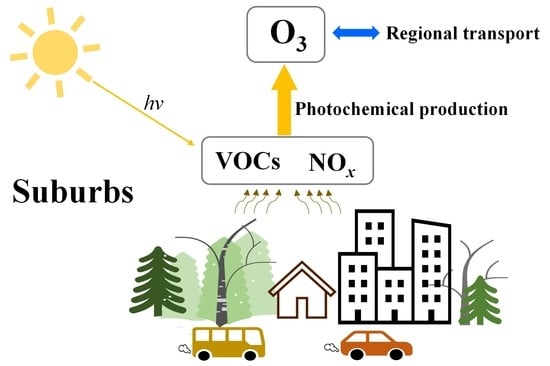
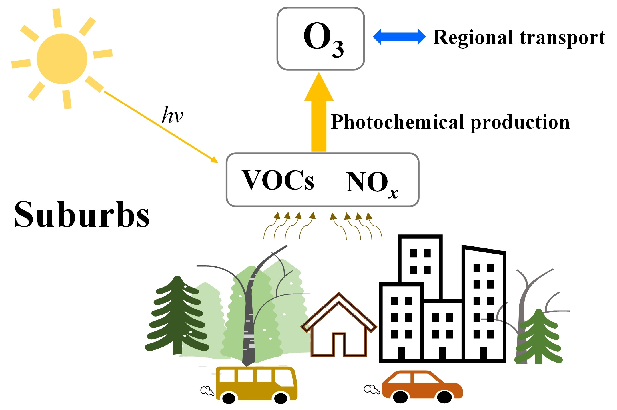
Investigation of Summertime Ozone Formation and Sources of Volatile Organic Compounds in the Suburb Area of Hefei: A Case Study of 2020

1
Laboratory of Atmospheric Physico-Chemistry, Anhui Institute of Optics and Fine Mechanics, HFIPS, Chinese Academy of Sciences, Hefei 230031, China
2
Science Island Branch, Graduate School, University of Science and Technology of China, Hefei 230026, China
3
School of Environmental Science and Optoelectronics Technology, University of Science and Technology of China, Hefei 230026, China
*
Authors to whom correspondence should be addressed.
Atmosphere 2023, 14(4), 740; https://doi.org/10.3390/atmos14040740
Submission received: 23 March 2023 / Revised: 13 April 2023 / Accepted: 15 April 2023 / Published: 19 April 2023
(This article belongs to the Special Issue Source Apportionment of Regional Ozone Pollution)

Abstract

:
Ground surface ozone (O3) is an emerging concern in China due to its complex formation process. In August 2020, field measurements of O3, NOx, and volatile organic compounds (VOCs) were carried out in Hefei’s western suburbs. The pollution features of VOCs and O3 formation were thoroughly analyzed. The total VOC concentration was 42.26 ppb, with the dominant contributor being oxygenated VOCs (OVOCs). Seven emission sources were recognized using the positive matrix factorization (PMF) model, including aged air masses, combustion sources, fuel evaporation, industrial emissions, vehicular emission, solvent utilization, and biogenic emission. Ozone generation mainly occurred under an NOx-limited regime based on the zero-dimensional box model analysis. According to the scenario analysis, the 13% cut in O3 might be achieved by the 10% and 30% reduction in NOx and VOCs, respectively. The O3 budget analysis demonstrates its high ozone production rate during the pollution period. The influence of regional transport cannot be ignored for high O3 pollution. This paper provides scientific evidence for O3 production and the strategies of reducing O3 by controlling its precursors.

Graphical Abstract

1. Introduction

Tropospheric ozone (O3) is an important air pollutant that harms human health and plant and animal growth [1,2]. It directly affects the climate and natural ecosystems [3]. In China, ground surface O3 concentrations have increased rapidly in many cities in recent years [4]. Lu et al. showed that the warm-season daily maximum 8 h average (MDA8) ozone levels from Chinese urban sites increased by 2.4 ppb year−1 between 2013 and 2019 [5]. Nevertheless, the formation mechanisms of O3 pollution are exceedingly complicated because of the complicated varieties and sources of its precursors [6,7]. Thus, mitigating O3 pollution has become vital for the promotion of ambient air quality in China.
O3 generation is affected by multiple factors, such as O3 precursors, atmospheric oxidation capacity, meteorological factors, and regional transport [8,9,10]. Generally, ground surface O3 is primarily produced from photochemical processes between volatile organic compounds (VOCs) and atmospheric radicles such as hydroxyl and nitrate in the presence of nitrogen oxides (NOx) and ammonia (NH3) [11,12]. In addition, during the night, O3 is consumed by biogenic VOCs, such as pinene and isoprene [13,14,15]. Over the past two decades, extensive studies have been performed exploring the influences of emissions and atmospheric processes on O3 pollution in China [16,17,18,19]. Most of them were focused on developed regions, such as the Beijing–Tianjin–Hebei (BTH) [10], Yangtze River Delta (YRD) [7], Pearl River Delta (PRD) [17], and Chengdu–Chongqing regions [18]. Those studies showed that ozone production was more likely to be under VOC-limited regimes in urban regions but NOx-limited regimes in rural regions in China [16]. However, O3 generation is much more complicated due to the non-linear relationship between VOCs and NOx. Therefore, in-depth identification of O3 and its precursors in the O3 pollution period is fundamental to fully understanding the O3 formation process.
Observation-based models (OBMs) and emission-based chemical transport models (EBMs) are widely used to investigate the non-linear relation of O3 and its precursors [20,21,22,23]. The EBM method is suitable for a large geographical scale [21,22], while the OBM approach mainly utilizes the local scale for in situ O3 formation chemistry analysis and has the advantage of using local online measurements [23]. For example, Liu et al. (2022) adopted OBM and found that the O3 episode period was the simultaneous action of regional transport and local photochemical generation in the coastal cities in China [24]. Li et al. (2023) applied the zero-dimensional (0-D) box model (an observation-based method) and revealed that O3 production regimes covered the VOC-limited, transitional, and NOx-limited regimes in the nearby oil fields of Shandong Province [25]. Furthermore, VOCs are critical precursors for the formation of ground-level O3, while there are significant geographical and seasonal variations in the distribution of VOCs in China [19]. Thus, the identification of VOC sources is essential for the implementation of O3 pollution control. The chemical mass balance method (CMB), principal component analysis (PCA), and positive matrix factorization (PMF) are common source apportionment technologies [26,27]. In these source apportionment technologies, PMF is considered the most efficient quantitative method [26]. PMF can weigh and conduct least squares tests of the data. The distinctive feature of the PMF is that non-negative source component spectra and source contribution can be obtained, and the analysis results are more reliable and meaningful for the source apportionment of environmental pollutants.
Hefei, located in the middle of the YRD, is the capital city of Anhui Province, whose economy and population have been growing rapidly in recent years. Like most other Chinese cities, its air quality has significantly improved in the last five years. The annual concentration of fine particulate matter (PM2.5) and sulfur dioxide (SO2) decreased, while the concentration of O3 increased. Compared with the annual concentrations of O3 in 2015, it increased by 41.6% in 2020 [28]. It is imperative to reveal the characteristics of ozone pollution. Previous studies have studied VOC and O3 pollution in the urban atmosphere of Hefei [29,30,31,32]. However, most focused on O3 spatiotemporal distributions, VOC sources, and the effect of meteorological conditions on ozone formation, with limited studies having been performed on the O3 precursor relationship in Hefei.
To better understand the chemical interactions of O3 and its precursors, a field campaign was conducted in the summer of 2020 at a suburban site in Hefei. The PMF model was used to deduce the emission sources of VOCs. A zero-dimensional box model was used to assess the in situ O3 photochemistry and its sensitivities to O3 precursors. These findings could help local governments implement effective strategies for the reduction of O3 and its precursors.

2. Materials and Methods

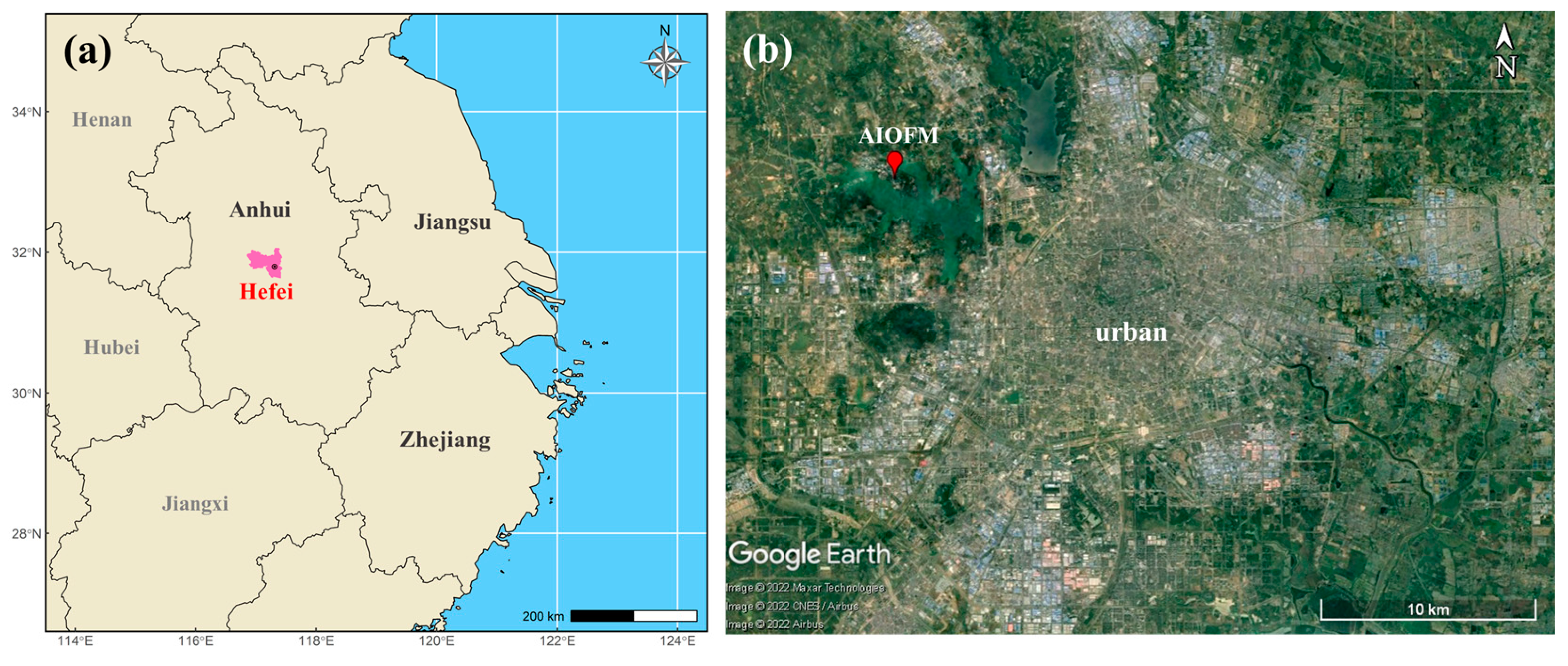
2.1. Observation Site Location

The observation was performed in the Anhui Institute of Optics and Fine Mechanics (AIOFM), Chinese Academy of Sciences (31°54′19″ N, 117°9′43″ E). This site is located on a peninsula near Shushan Lake in the western suburb of Hefei, approximately 10 km from downtown (Figure 1), and it is surrounded by water on three sides and sheltered by shrubs and trees. The sampling was conducted from 18 August to 2 September 2020.

2.2. Measurement of VOCs and Other Air Pollutants

In this study, VOCs were sampled on the top of the 7th floor of the building in AIOFM, nearly 20 m above the ground. Sixteen VOC samples were collected each day. The specific sampling intervals were 1 hour during the daytime (07:00–19:00) and 3 h at night (19:00–07:00). Each sample was collected in a 3.2 L stainless steel canister (Entech Instrument Inc., Simi Valley, CA, USA) with a flow restrictor (CS1200E series, Entech Instrument Inc., Simi Valley, CA, USA).
The VOC samples were treated using a preconcentrator (Model 7200, Entech Instruments Inc., Simi Valley, CA, USA) combined with a gas chromatography system equipped with a mass spectrometer and a flame ionization detector (GC–MS/FID). The details of the analytical process are described in Text S1. A total of 116 VOC species were measured, including 29 alkanes, 11 alkenes, 1 alkyne, 18 aromatics, 35 halocarbons, 21 OVOCs, and carbon disulfide. VOC species information is listed in Table S1.
Additionally, the meteorological parameters (total solar irradiance, temperature, relative humidity, pressure, wind speed, and wind direction) and trace gas concentrations (SO2, NO, NO2, CO, O3, PM10, and PM2.5) were collected from the Dongpu Reservoir’s air quality monitoring station (http://sthjj.hefei.gov.cn/, accessed on 1 October 2020), which is installed on the 6th floor of a building in AIOFM.

2.3. Source Identification

PMF version 5.0 software [26,33] was used to determine potential VOC sources. The basic formulas for PMF calculation are as follows:
x i j = k = 1 p g i k f k j + e i j
where xij is the concentration of species j measured on sample i, p is the number of factors, fkj is the concentration of species j in factor profile k, gik is the relative contribution of profile k to sample i, and eij is the error for the j species measured on sample i. The gik and fkj are modified until a minimum Q value for a specified p is obtained. Q is defined as follows:
Q = i = 1 n j = 1 m e i j σ i j 2
where σij is the uncertainty of the jth species concentration in sample i, n is the number of samples, and m is the number of species. Details about the PMF model are summarized in the Supplementary Materials (Text S2).

2.4. 0-D Box Model Analysis

To simulate how VOCs contribute to photochemical O3 formation, a Framework for 0-D Atmospheric Modeling (F0AM) based on the Master Chemical Mechanism (MCM3.3.1) was used in this study [25,34]. The observed meteorological parameters (T, P, and RH) and gaseous pollutants (i.e., O3, CO, SO2, NO, NO2, VOCs) were input into the F0AM as constraints.
Photochemical ozone production in the troposphere can be calculated from the oxidation rate of NO to NO2 by peroxyl radicals (HO2, RO2). Based on the model output, the radical concentrations were used to quantify the generation and destruction pathways of ozone as follows:
G ( O 3 ) = k NO + HO 2 [ NO ] [ HO 2 ] + [ NO ] i k i [ RO 2 ] i  
D ( O 3 ) = k O 1 D + H 2 O [ O ( 1 D ) ] [ H 2 O ] + k O 3 + Alkene [ O 3 ] [ Alkene ] + k O 3 + OH [ O 3 ] [ OH ]
+ k O 3 + HO 2 [ O 3 ] [ HO 2 ] + k NO 2 + OH [ NO 2 ] [ OH ]
P(O3) = G(O3) − D(O3)
where G(O3) is the gross O3 production rate, D(O3) is the ozone chemical loss rate, P(O3) is the net O3 production rate, and k represents the related reaction rate constant. Detailed descriptions of the chemistry calculation can be found elsewhere [24,25].
The relative incremental reactivity (RIR) was used to calculate the sensitivity of ozone production to its precursors, and it is defined by the following equation:
RIR = Δ P ( O 3 ) / P ( O 3 ) Δ X / X
where X is the specific O3 precursor, ΔP(O3)/P(O3) is the percentage change in the ozone production rate, ∆X/X is the fraction of ozone precursors reduction, in this study, a hypothetical relative change (∆X/X) of 20% was set. A positive RIR value indicates that reducing emissions of the target precursor is effective in reducing O3 production, and the larger the positive value, the more sensitive to the target precursor for O3 formation [25].
The Empirical Kinetics Modeling Approach (EKMA) curve is an important tool for diagnosing the sensitivity of zone formation to VOCs and NOx. The O3 concentration was simulated by setting different VOCs and NOx mixing ratios. We set up a 20 × 20 matrix by reducing or increasing the measured VOCs and NOx concentrations in the model input. The ozone concentration was modeled with intervals of 24 h spanning from 0:00 to 23:00 at a 1 h time resolution. The maximum daily O3 concentration (06:00–18:00) can be obtained using various concentrations of NOx and VOCs. Finally, the O3 maximum concentration was plotted under the corresponding scenarios to generate an EKMA curve. In this study, S(NOx), S(VOCs), and S(O3) correspond to concentrations of NOx, VOCs, and O3, respectively.

3. Results and Discussion

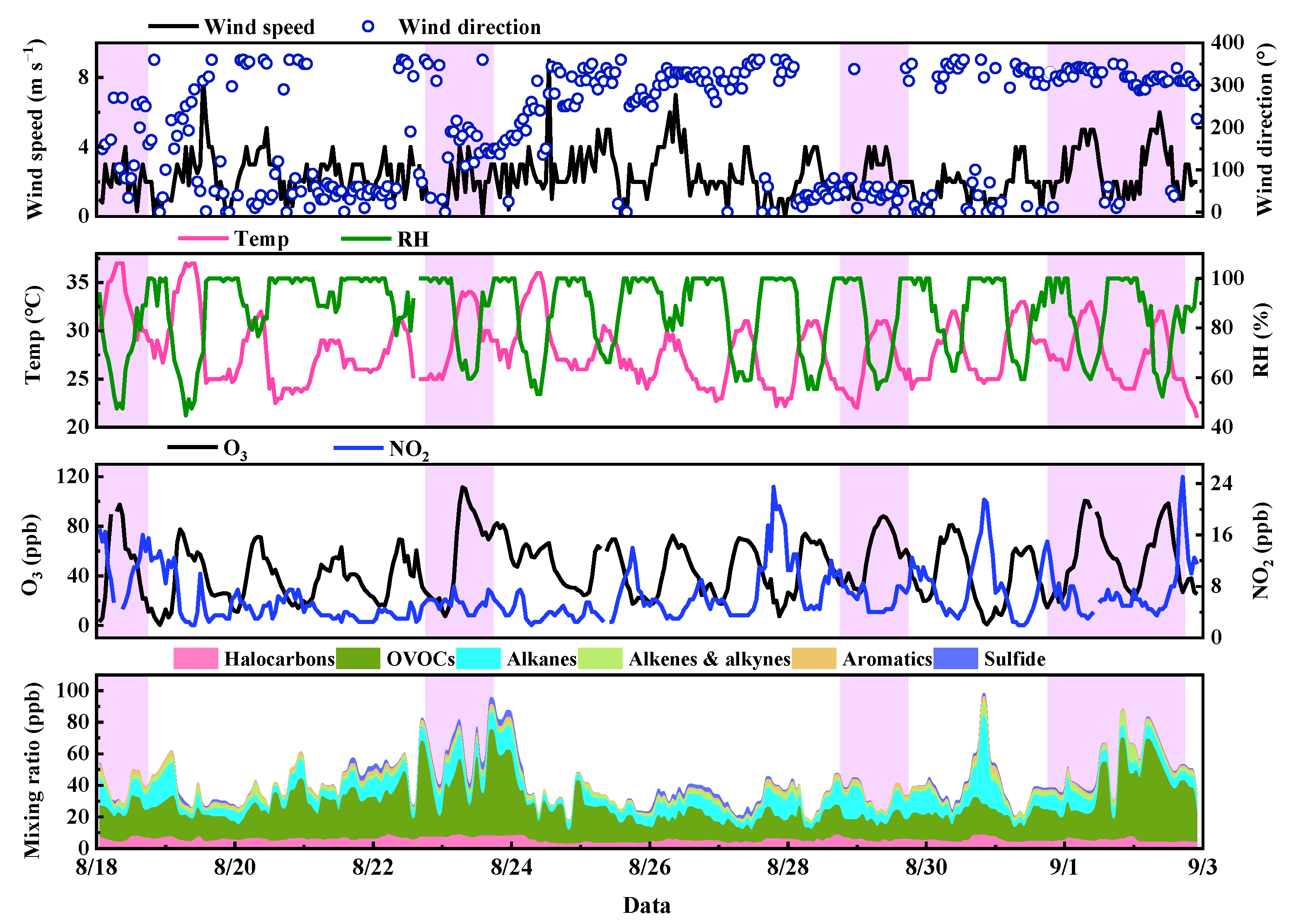
3.1. Overview of Meteorology and Pollutants Characteristics

3.1.1. Levels of Air Pollutants and Meteorological Factors

Figure 2 shows the meteorological parameters, O3 concentrations, and precursor time series observed from 18 August to 2 September 2020. During the campaign, the average T, RH, and wind speed were 27.94 °C, 86.1%, and 2.31 m s−1, respectively, with the prevailing wind direction coming from the northeast. The mixing ratio of O3 changed greatly, and its concentration ranged from 0.5 ppb to 110 ppb, with a mean value of 45.66 ppb. According to the specification for stage II of the Chinese National Ambient Air Quality Standards (NAAQS) [35], the MDA8 of O3 concentration is 160 µg m−3, which is comparable to 75 ppb under the typical summer conditions (25 °C, 101.3 kPa). As shown in Figure 2, two cases of different O3 pollution levels were chosen to study the characteristics of VOCs and O3. The dates when the MDA8-O3 mixing ratio was greater than 75 ppb were classified as O3 episode days, and the remaining dates were non-O3 episode days.
The time profiles of the VOC groups in this study are depicted in Figure 2. The average total TVOCs (TVOCs) mixing ratio was 42.26 ppb. The average concentrations of OVOCs, alkanes, halogenated hydrocarbons, alkenes and alkynes, aromatic hydrocarbons, and sulfide were 22.13, 8.99, 5.63, 2.62, 1.61, and 1.3 ppb, respectively. They accounted for 52.4%, 21.3%, 13.3%, 6.2%, 3.8%, and 3% of the total detected VOCs, respectively. A comparison of the results with different cities in China is listed in Table 1. The concentration of TVOCs in Hefei’s suburbs was higher than that in Zhengzhou (29.11 ppb) [27], Yibin (23 ppb) [36], Xi’an (29.1 ppb) [37], and Guilin (23.67 ppb) [38], comparable to Shanghai (42.7 ppb) [39], and lower than Guangzhou (76.84 ppb) [40] and Ningde (49.1 ppb) [19]. OVOCs were the main components of VOCs in this study, in contrast to other cities in China where alkanes were the largest contributor to VOC species. The high mixing ratio of OVOCs in summer Hefei was similar to that observed in Zhengzhou [27] and Guangzhou [40].

3.1.2. Diurnal Variation Characteristics

Diurnal variations for diffident O3 pollution levels at the AIOFM site are shown in Figure 3 and Figure S1. During the O3 pollution days, there was a relatively higher total solar irradiance (TSI), temperature and lower relative humidity than during non-O3 pollution periods, which is consistent with previous observations that high solar radiation and temperature and low relative humidity could promote ozone generation [25,41]. The diurnal profile of O3 shows an inverse variation trend with NO2 and VOC groups. The peak values of ozone were 94.2 ppb (O3 pollution period) and 63.68 ppb (non-O3 pollution period) in the two periods, respectively. The observational results demonstrate that increased O3 concentrations are related to stronger solar radiation, high temperature, low relative humidity, and higher precursor concentrations.
Generally, the diurnal profile of VOCs in the atmosphere is characterized by direct emissions, consumption by atmospheric oxidants, and boundary layer height (BLH) variations [42]. Increased anthropogenic activities in the morning resulted in VOC accumulation. The VOCs gradually decreased with the increase in the photochemical reaction and BLH (Figure S1). When the photochemical reaction stops in the evening, the concentration of VOCs rises due to the influence of emissions. As anthropogenic emissions species, benzene, and propane demonstrated consistent daily variation with multiple peaks, which is in agreement with the diurnal profiles of NO2 (Figure 3). The first peak occurs in the early morning, typical of traffic source emissions. As the typical tracer for biogenic emission, isoprene showed good consistency with the diurnal profiles of temperature and solar radiation (Figure S1). As shown in Figure 3, it was clear that the nighttime and morning VOC mixing ratios during the O3 pollution days were higher than those during the non-O3 pollution period. This suggested that the high mixing ratios of VOCs gathered at night and morning might be prime reasons for the increasing O3 concentration.
Table 2 shows that all VOC groups increased continuously during the O3 period except for carbon disulfide. Alkanes, aromatic hydrocarbons, alkenes and alkynes, halogenated hydrocarbons, and OVOCs increased by 16.9%, 20.1%, 24.1%, 13.1%, and 36.7% on the O3 episode days, respectively. The concentration of OVOCs increased the most, with an average concentration of 27.53 ppb during the pollution period, accounting for 55% of the total detected VOCs. As with the features of the whole campaign, OVOCs were the most abundant components in both non-O3 and O3 pollution days. Except for direct emissions, OVOCs can also be generated by chemical reactions from the oxidation of their precursor hydrocarbons [43]. Moreover, the mean concentrations of NO2, O3, PM2.5, and PM10 on the O3 episode days were 6.94 ppb, 55.54 ppb, 60.06 µg m−3, and 44.84 µg m−3, respectively (Table 2). Compared with the non-O3 pollution period, NO2, O3, PM2.5, and PM10 increased by 10.4%, 33.6%, 50.7%, and 34%, respectively. Thus, high concentrations of precursors and increased atmospheric oxidation may lead to more secondary components, such as OVOCs, O3, and PM2.5.

3.2. Source Apportionment of VOCs

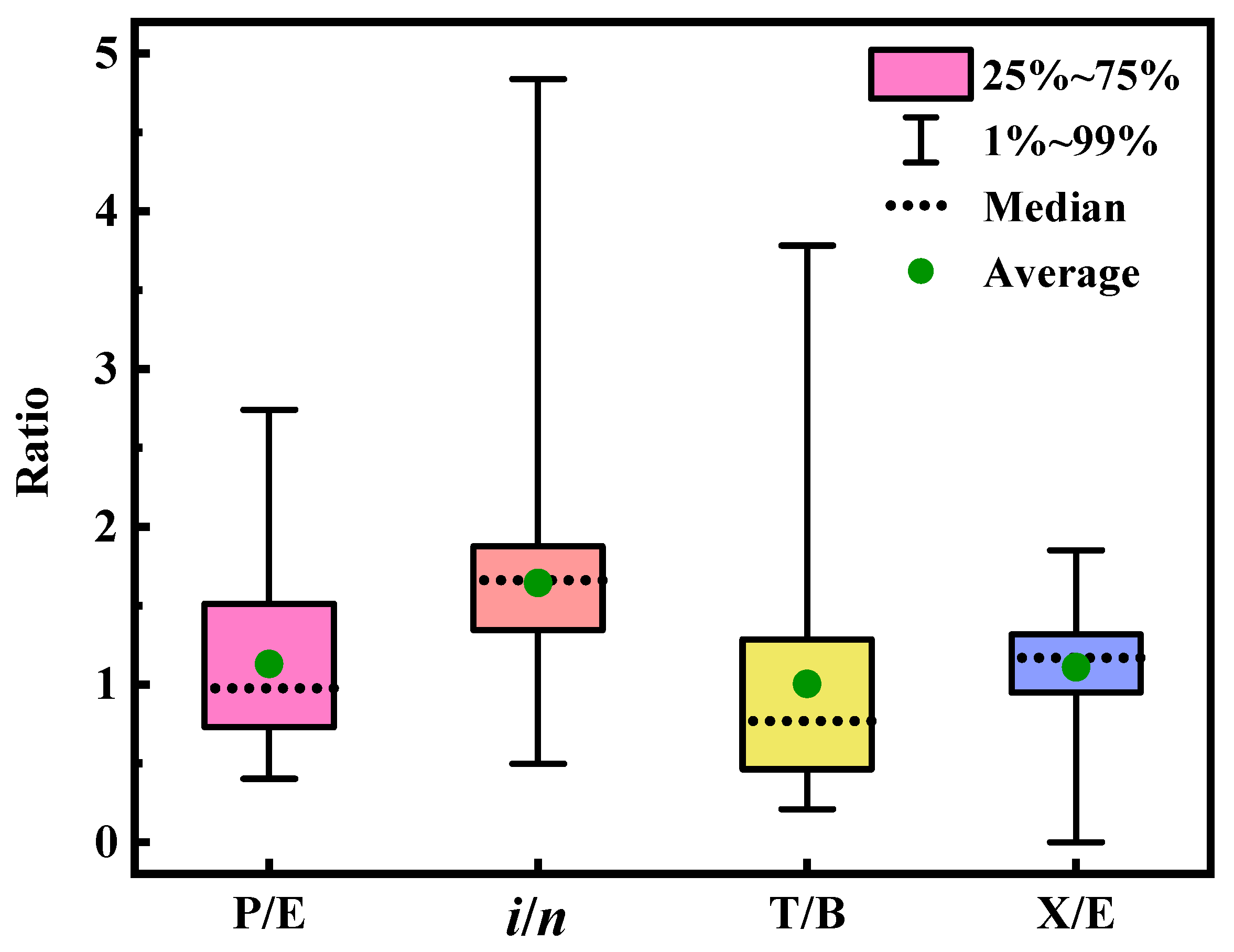
3.2.1. Ratio of Specific Compounds
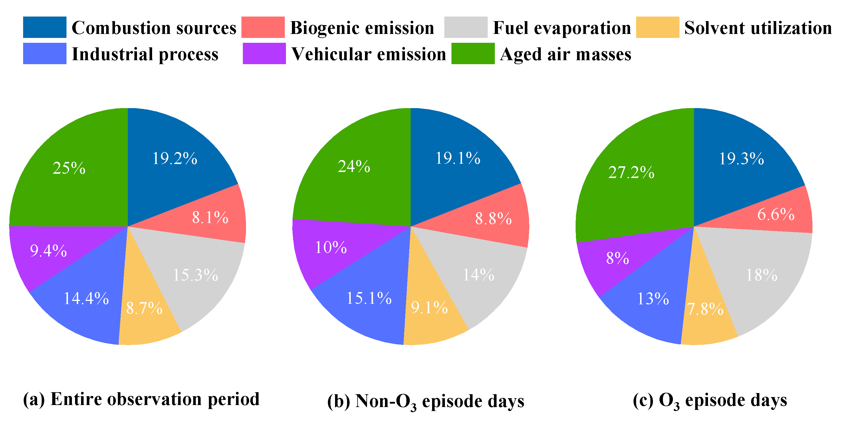
The ratios between specific VOCs can reflect different sources. The most commonly used ratios are propane/ethane (P/E), i-pentane/n-pentane (i/n), m/p-xylene/ ethylbenzene (X/E), and toluene/benzene (T/B) [19,38]. The P/E ratio is frequently used to assess the impacts of liquefied petroleum gas/natural gas (LPG/NG) use on VOCs [44,45]. As shown in Figure 4, the average P/E ratio in this study was 1.66 ± 0.64, lower than that in LPG/NG vehicle exhaust (about 3) [46], indicating that propane was also affected by other emission sources. The i/n ratio is 0.56~0.8 for coal burning, 1.8~4.6 for fuel evaporation, and 2.2~3.8 for vehicle exhaust emission [19,47]. As shown in Figure 4, the i/n ratio during the observation period was mainly distributed between 1.34~1.88, with a mean value of 1.66 ± 0.64, suggesting that alkanes near the sampling site were related to fuel evaporation emission.
The T/B ratio at about 0.3 is for combustion sources, 0.9~2.2 for vehicle exhaust, and 1.4~5.8 for solvent usage sources [37,48,49]. As depicted in Figure 4, the T/B ratio was mainly distributed between 0.46~1.29, with an average value of 1.0 ± 0.77, indicating that the VOCs near the sampling site had the characteristics of combustion and traffic source emissions. However, the correlation between toluene and benzene was poor (Figure S2), with a correlation coefficient (R2) of 0.15, suggesting that the sources of toluene and benzene differed significantly. The X/E ratio is often used to indicate the degree of air mass aging [50,51,52]. The small X/E ratio revealed a high degree of air mass aging, which could be attributed to the influence of air mass transport. Generally, an X/E ratio in the range of 2.5~2.9 is an attribute of typical urban environments. If the ratio is much smaller than 2.9, the VOCs are impacted greatly by long-distance transmission [53,54]. The correlation coefficient between m/p-xylene and ethylbenzene in this study was 0.74 (Figure S2), implying that the VOC sources had a high consistency. As demonstrated in Figure 4, the average value of X/E was 1.11 ± 0.36, much lower than 2.9, highlighting the role of long-distance transport in VOC sources.

3.2.2. PMF Analysis

PMF 5.0 software was used for source analysis in this study. The OVOCs and alkenes with high chemical activities can be greatly affected by the secondary formation. These pollutants were excluded from the PMF analysis [55]. The Supplementary Materials show the factor screening and error analysis for the source analysis model (Text S2). Seven VOC sources were identified: combustion, biogenic emission, fuel evaporation, solvent utilization, industrial process, vehicular emission, and aged air masses. Details characterizations are provided in Figure S1 and Text S3.
Figure 5 shows the proportion of various sources according to the PMF results. The aged air masses made the largest contributions, accounting for 25% of atmospheric VOCs. The combustion sources, fuel evaporation, and industrial emission were also relatively high, contributing 19.2%, 15.3%, and 14.4%, respectively. The vehicular emission, solvent utilization, and biogenic emission contribution were relatively low at 9.4%, 8.7%, and 8.1%, respectively. Furthermore, the contributions of various sources did not differ significantly at different ozone pollution levels. Compared with the non-O3 pollution period, the contributions of aged air masses and the combustion sources increased only by 3.2% and 4%, respectively. The proportion of industrial and biogenic emissions decreased by 2.1% and 2.2%, respectively. However, the mixing ratio of each source increased significantly, except for biogenic emissions. The mixing ratio of combustion sources, aged air masses, and fuel evaporation increased by 38%, 29.6%, and 21.3%, respectively.

3.3. Photochemical O3 Formation and Regional Transport

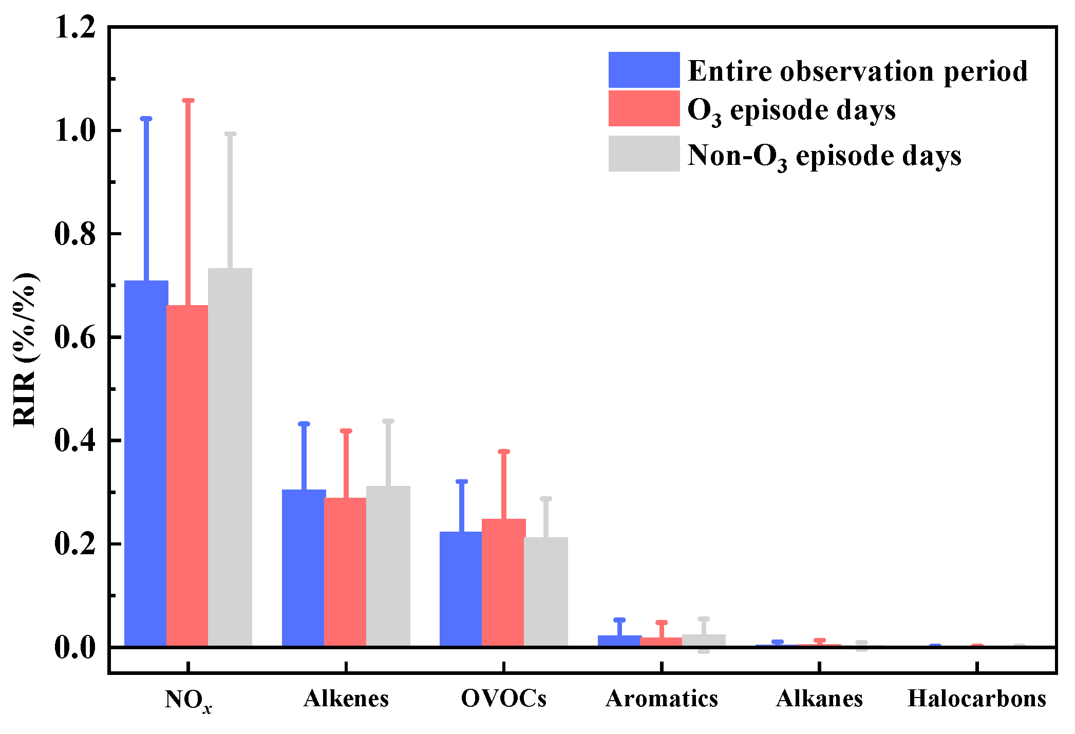
3.3.1. Sensitivity Analysis of Ozone Formation

The ozone generation process was simulated by F0AM–MCM to diagnose the sensitivity of ozone generation to its precursors in this study. The RIR values of the O3 precursors corresponding to the different ozone pollution levels are shown in Figure 6. The RIR value of NOx is the greatest, followed by alkenes, OVOCs, aromatics, alkanes, and halocarbons. The RIR values of VOCs and NOx were both positive during the campaign. This revealed that reducing all precursors could benefit overall O3 regulation in summer in Hefei’s suburbs. Moreover, the RIR value for OVOCs increased during the ozone episode days, implying that reducing OVOCs might reduce O3 pollution on high O3 days. The high fraction of alkenes and OVOCs in RIR values suggests that ozone control in Hefei’s suburbs should be performed in consideration of such VOC species in the summer.
Figure 7 depicts O3-VOCs-NOx sensitivity using the EKMA curve. A total of 400 scenarios were performed, assuming that 20 emission scenarios were for NOx and VOCs. The photolysis rates and meteorological conditions for all the scenarios were based on the average conditions during the whole campaign. The maximum O3 concentration (06:00–18:00) modeled is depicted with spots of various colors on the corresponding Z-axis. The black line is the ridgeline, formed by the turning point of the O3 isopleth. Ozone production is NOx-limited below the ridgeline and VOC-limited above the ridgeline, with a transition region near the ridgeline. As depicted in Figure 7, the slope of the ridgeline is approximately 3 (VOCs/NOx), which provides a scientific basis for O3 control policies in reducing VOCs and NOx emissions [56]. The daily average concentrations of VOCs and NOx were plotted in the EKMA curve. Most of those were below the ridgeline, indicating that ozone formation is significantly affected by NOx at the AIOFM site, which is consistent with those found in the other suburban regions in China [57,58]. However, Figure 7 also shows that several spots were scattered close to the ridgeline in the EKMA curve (18 August and 28 August), indicating that reducing NOx alone was not the most effective strategy for cutting O3.

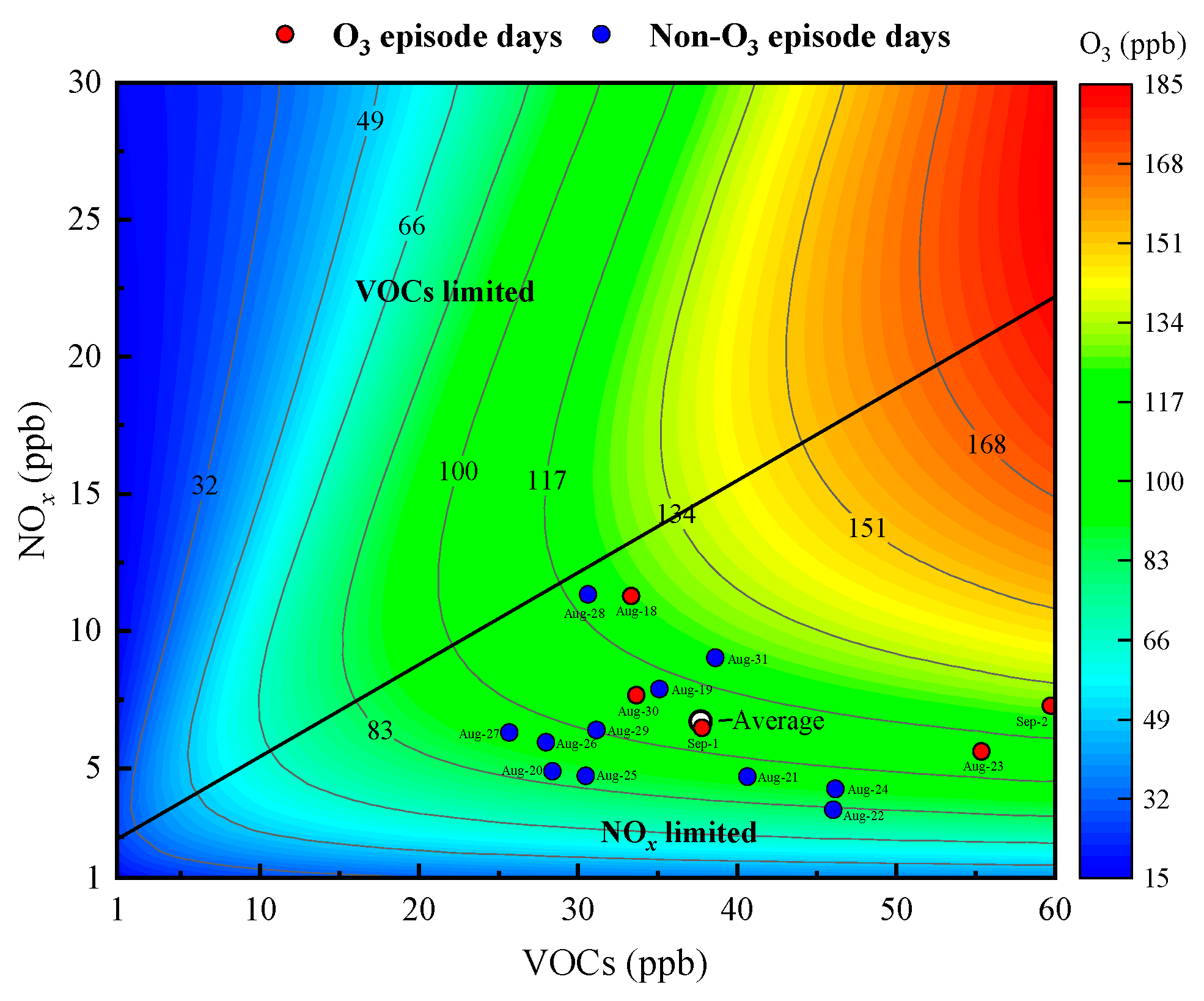
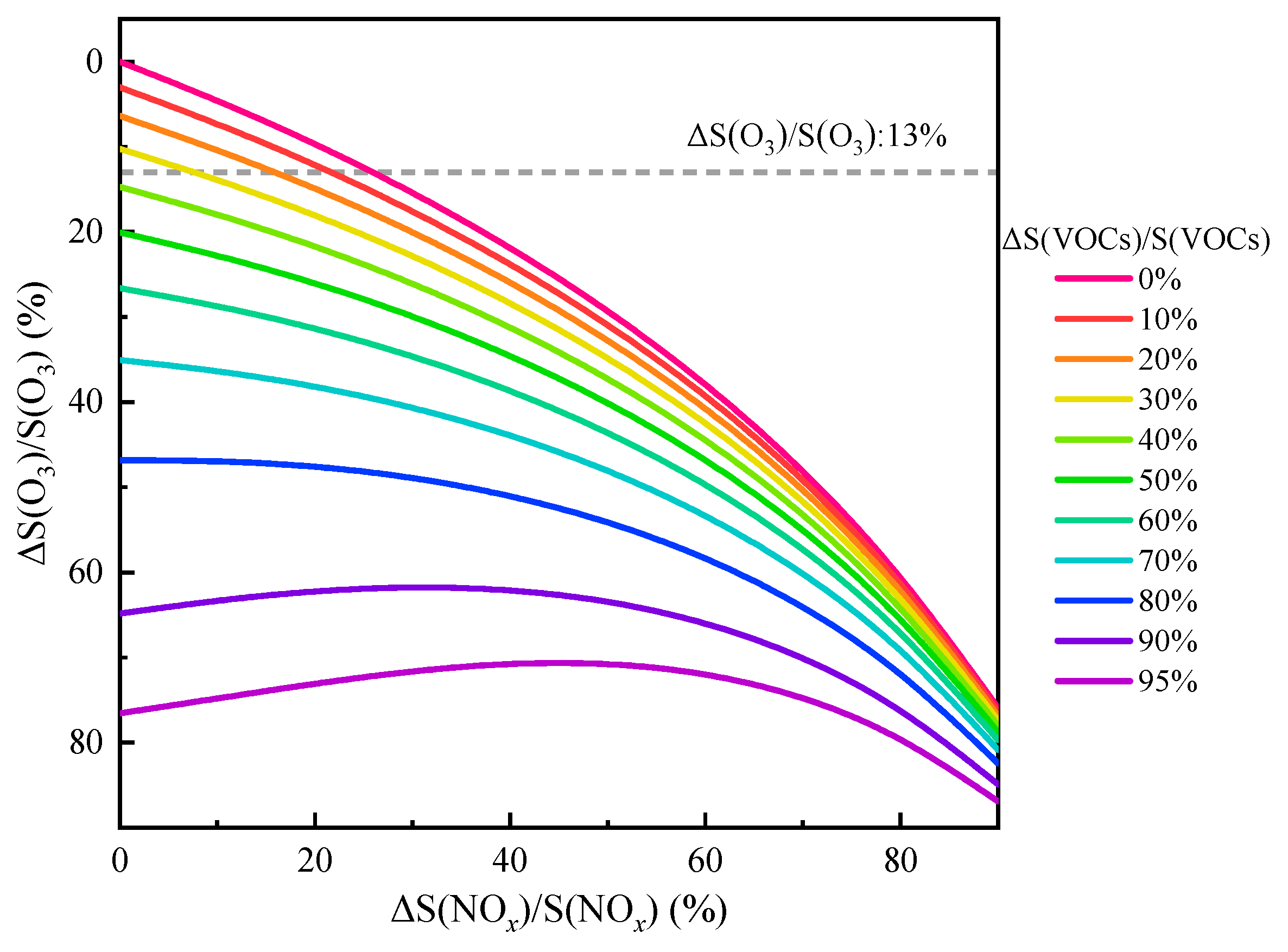
3.3.2. O3 Control Strategies

In order to investigate O3 control policies during the O3 episode days, F0AM–MCM was used to simulate different scenarios with reductions of VOCs and NOx. The EKMA results showed that ozone generation was more sensitive to NOx during the whole campaign, which is compatible with the results of the RIR analysis. Furthermore, the MDA8h of the O3 mixing ratio during the O3 episode days was 85.4 ppb, exceeding stage II of the NAAQS of 75 ppb for O3 by 13%. As shown in Figure 8, the 13% ozone cut goal was achieved with the 26% mitigation of S(NOx) and the S(VOCs), maintaining the initial emission. NOx emission reduction might be efficient for reaching short-term O3 attainment in local areas. However, considering the results of RIR and EKM analyses, and full compliance with the long-term multi-pollutant air quality improvement strategy in China, VOCs should be properly decreased, since they are important precursors of SOA; to reach the 13% reduction of O3, a more practical and reasonable way would be to reduce S(VOCs) and S(NOx) by 30% and 10%, respectively (Figure 8). Moreover, the reduction ratio of VOCs/NOx follows the ridgeline in the EKMA curve (Figure 7). In general, some conclusions and suggestions were drawn for the short observation period, and longer-term field measurements of air pollutants should be performed in the future. Simultaneously, it is crucial to properly adapt the mitigation of VOCs and NOx policies when O3 formation sensitivity changes.

3.3.3. In Situ O3 Formation Process

Variations in O3 concentration depend on the local photochemical production and physical transport processes [10,59,60]. Thus, the impact on O3 concentrations of photochemical and physical transport processes can be expressed as follows:
d ( O x ) d t = P ( O 3 ) + R ( O 3 )
where d(Ox)/dt is the observed rate of change in O3, P(O3) is the net O3 formation rate, and R(O3) is the regional transport rate. P(O3) can be computed by the F0AM. O3 was replaced with Ox (Ox = O3 + NO2) to correct the titration of O3 by NO [61]. The positive R(O3) values indicated the O3 import of regional transport and vice versa [24,61].
The results of the ozone budget analysis conducted at the AIOFM site are shown in Figure 9. The d(Ox)/dt shows a similar increase in the morning during the O3 and non-O3 episodes. Compared with the O3 pollution period, a positive d(Ox)/dt is observed at 06:00, 1 h earlier than the non-O3 pollution period. Moreover, the increase rate of Ox is the fastest during the O3 pollution period in the morning hours, and it remains positive until 14:00, while the d(Ox)/dt sharply decreases to zero at 13:00 during the non-O3 pollution period. The difference in the d(Ox)/dt results in a high O3 peak during the O3 pollution period.
As shown in Figure 9, the maximum values of P(O3) were 13 ppb h−1 (O3 pollution period) and 7.31 ppb h−1 (non-O3 pollution period) at around 09:00, respectively, and the increase in the Ox mixing ratio is close to the local ozone production rate, indicating that the fast O3 mixing ratio increase in the morning (around 06:00–09:00) is mainly caused by local photochemical production. However, both positive R(O3) values for the different pollution periods were observed at around 09:00–12:00, indicating that the local ozone budget was O3 importing. Specifically, during the O3 pollution period, the R(O3) values at 10:00 and 11:00 were 8.46 ppb h−1 and 7.31 ppb h−1, respectively. They are responsible for 47.9% and 50.9% of the d(Ox)/dt, respectively. This result indicated that the high O3 formation was caused by the interaction of physical transport and local photochemical production in the studying area. The Ox is probably emitted from the residual layer, which holds the high Ox load generated on the earlier day and then separated from the surface layer [59].
The O3 import stops (negative R(O3)) at around 13:00 during the O3 pollution period, while the local photochemical production kept producing O3, it showed that the downwind regions as well as the in situ O3 concentration were both influenced by the local photochemical production at the studying site. This can be further observed in Figure 9a under high-O3 conditions. Overall, these results indicate that regional transport and local photochemical production played significant roles during the O3 pollution period.

4. Conclusions

In this study, comprehensive field observations were conducted in the western suburbs of Hefei from 18 August to 2 September 2020. A total of 116 VOC species were monitored, and the mixing ratio of TVOCs was 42.26 ppb. OVOCs were the most abundant group, followed by alkanes. Compared with the non-O3 pollution period, enhanced solar radiation, high temperature, and low humidity conditions were observed during the O3 pollution period. Meanwhile, the mixing ratios of NOx and VOCs increased significantly. Those conditions led to greater formation of secondary pollutants.
The average X/E ratio during the campaign was 1.11, with a high degree of air mass aging, suggesting that regional transportation had a major impact on VOCs. Seven sources were recognized by the PMF model, including aged air masses (25%), combustion sources (19.2%), fuel evaporation (15.3%), industrial emission (14.4%), vehicular emission (9.4%), solvent utilization (8.7%), and biogenic emission (8.1%). The contributions of each source were comparable under different O3 episode days. However, the mixing ratio of each source greatly increased, except for biogenic emission during the O3 pollution period.
Based on the RIR and EKMA analyses, the ozone generation in summer in the western suburbs of Hefei was more sensitive to NOx, with alkenes and OVOCs as the major contributors to O3 formation. The F0AM–MCM-simulated results illustrated that a 10% diminution of S(NOx) and 30% diminution of S(VOCs) may result in a 13% diminution of S(O3) during the O3 episode days. The in situ O3 generation process results demonstrated that regional transport and local photochemical production aggravated local O3 concentration.

Supplementary Materials

The following supporting information can be downloaded at: https://www.mdpi.com/article/10.3390/atmos14040740/s1, Text S1: Analytical process for GC–MS/FID; Text S2: Detail procedure for positive matrix factorization (PMF); Text S3: The introduction of different VOC sources; Table S1: The species information of VOCs measured at the AIOFM site; Table S2: The results of base bootstrap at the AIOFM site; Figure S1: Diurnal variations of SO2, CO, NO, total solar irradiance (TSI), boundary layer height (BLH), propane, isoprene, benzene, and acetone during the non-O3 and O3 episode days; Figure S2: Linear correlations (R2) between (a) propane/ethane, (b) i-pentane/n-pentane, (c) m/p-xylen/o-xylene, (d) toluene/benzene during the observation period; Figure S3: Source profiles and contribution percentages from each source during the observation period by the PMF model. References [62,63,64,65,66] are cited in Supplementary Materials.

Author Contributions

Data formal analysis, writing—original draft preparation, H.Y.; sampling, Q.L., M.H.; investigation, S.W.; review and editing, N.W., J.Z., Q.L.; funding acquisition, X.X., W.Z. (Weixiong Zhao); supervision, W.Z. (Weijun Zhang). All authors have read and agreed to the published version of the manuscript.

Funding

This research was funded by the National Natural Science Foundation of China (Grant No. U21A2028 and 42105099), the National Research Program for Key Issues in Air Pollution Control, China (Grant No. DQGG202117), the Youth Innovation Promotion Association CAS (Grant No. Y202089), and the HFIPS Director’s Fund (Grant No. YZJJ202101).

Institutional Review Board Statement

Not applicable.

Informed Consent Statement

Not applicable.

Data Availability Statement

Data available on request from the authors.

Acknowledgments

We are grateful for financial support from the National Natural Science Foundation of China (Grant No. U21A2028 and 42105099), the National Research Program for Key Issues in Air Pollution Control, China (Grant No. DQGG202117), the Youth Innovation Promotion Association CAS (Grant No. Y202089), and the HFIPS Director’s Fund (Grant No. YZJJ202101).

Conflicts of Interest

The authors declare that they have no known competing financial interests or personal relationships that could have appeared to influence the work reported in this paper.

References

  1. Lu, X.; Hong, J.; Zhang, L.; Cooper, O.R.; Schultz, M.G.; Xu, X.; Wang, T.; Gao, M.; Zhao, Y.; Zhang, Y. Severe surface ozone pollution in China: A global perspective. Environ. Sci. Technol. Lett. 2018, 5, 487–494. [Google Scholar] [CrossRef]
  2. Ivatt, P.D.; Evans, M.J.; Lewis, A.C. Suppression of surface ozone by an aerosol-inhibited photochemical ozone regime. Nat. Geosci. 2022, 15, 536–540. [Google Scholar] [CrossRef]
  3. Fu, T.-M.; Tian, H. Climate Change Penalty to Ozone Air Quality: Review of Current Understandings and Knowledge Gaps. Curr Pollution Rep. 2019, 5, 159–171. [Google Scholar] [CrossRef]
  4. Li, K.; Jacob, D.J.; Liao, H.; Shen, L.; Zhang, Q.; Bates, K.H. Anthropogenic drivers of 2013−2017 trends in summer surface ozone in China. Proc. Natl. Acad. Sci. USA 2019, 116, 422–427. [Google Scholar] [CrossRef] [PubMed]
  5. Lu, X.; Zhang, L.; Wang, X.; Gao, M.; Li, K.; Zhang, Y.; Yue, X.; Zhang, Y. Rapid increases in warm-season surface ozone and resulting health impact in China since 2013. Environ. Sci. Technol. Lett. 2020, 7, 240–247. [Google Scholar] [CrossRef]
  6. Wang, Z.; Tian, X.; Li, J.; Wang, F.; Liang, W.; Zhao, H.; Huang, B.; Wang, Z.; Feng, Y.; Shi, G. Quantitative evidence from VOCs source apportionment reveals O3 control strategies in northern and southern China. Environ. Int. 2023, 172, 107786. [Google Scholar] [CrossRef]
  7. Lyu, X.; Guo, H.; Zou, Q.; Li, K.; Xiong, E.; Zhou, B.; Guo, P.; Jiang, F.; Tian, X. Evidence for reducing volatile organic compounds to improve air quality from concurrent observations and in situ simulations at 10 stations in eastern China. Environ. Sci. Technol. 2022, 56, 15356–15364. [Google Scholar] [CrossRef]
  8. Meng, X.; Jiang, J.; Chen, T.; Zhang, Z.; Lu, B.; Liu, C.; Xue, L.; Chen, J.; Herrmann, H.; Li, X. Chemical drivers of ozone change in extreme temperatures in eastern China. Sci. Total Environ. 2023, 874, 162424. [Google Scholar] [CrossRef]
  9. Karl, T.; Lamprecht, C.; Graus, M.; Cede, A.; Tiefengraber, M.; Vila-Guerau de Arellano, J.; Gurarie, D.; Lenschow, D. High urban NOx triggers a substantial chemical downward flux of ozone. Sci. Adv. 2023, 9, eadd2365. [Google Scholar] [CrossRef]
  10. Ma, W.; Feng, Z.; Zhan, J.; Liu, Y.; Liu, P.; Liu, C.; Ma, Q.; Yang, K.; Wang, Y.; He, H.; et al. Influence of photochemical loss of volatile organic compounds on understanding ozone formation mechanism. Atmos. Chem. Phys. 2022, 22, 4841–4851. [Google Scholar] [CrossRef]
  11. Hao, L.; Kari, E.; Leskinen, A.; Worsnop, D.R.; Virtanen, A. Direct contribution of ammonia to α-pinene secondary organic aerosol formation. Atmos. Chem. Phys. 2020, 20, 14393–14405. [Google Scholar] [CrossRef]
  12. Babar, Z.B.; Park, J.-H.; Lim, H.-J. Influence of NH3 on secondary organic aerosols from the ozonolysis and photooxidation of α-pinene in a flow reactor. Atmos. Environ. 2017, 164, 71–84. [Google Scholar] [CrossRef]
  13. Iyer, S.; Rissanen, M.P.; Valiev, R.; Barua, S.; Krechmer, J.E.; Thornton, J.; Ehn, M.; Kurtén, T. Molecular mechanism for rapid autoxidation in α-pinene ozonolysis. Nat. Commun. 2021, 12, 878. [Google Scholar] [CrossRef] [PubMed]
  14. Babar, Z.B.; Park, J.-H.; Kang, J.; Lim, H.-J. Characterization of a smog chamber for studying formation and physicochemical properties of secondary organic aerosol. Aerosol Air Qual. Res. 2016, 16, 3102–3113. [Google Scholar] [CrossRef]
  15. Iinuma, Y.; Müller, C.; Berndt, T.; Böge, O.; Claeys, M.; Herrmann, H. Evidence for the existence of organosulfates from β-pinene ozonolysis in ambient secondary organic aerosol. Environ. Sci. Technol. 2007, 41, 6678–6683. [Google Scholar] [CrossRef] [PubMed]
  16. Wang, X.; Yin, S.; Zhang, R.; Yuan, M.; Ying, Q. Assessment of summertime O3 formation and the O3-NOx-VOC sensitivity in Zhengzhou, China using an observation-based model. Sci. Total Environ. 2022, 813, 152449. [Google Scholar] [CrossRef]
  17. Yang, L.; Luo, H.; Yuan, Z.; Zheng, J.; Huang, Z.; Li, C.; Lin, X.; Louie, P.K.K.; Chen, D.; Bian, Y. Quantitative impacts of meteorology and precursor emission changes on the long-term trend of ambient ozone over the Pearl River Delta, China, and Implications for Ozone Control Strategy. Atmos. Chem. Phys. 2019, 19, 12901–12916. [Google Scholar] [CrossRef]
  18. Ren, J.; Guo, F.; Xie, S. Diagnosing ozone–NOx–VOC sensitivity and revealing causes of ozone increases in China based on 2013–2021 satellite retrievals. Atmos. Chem. Phys. 2022, 22, 15035–15047. [Google Scholar] [CrossRef]
  19. Chen, G.; Liu, T.; Ji, X.; Xu, K.; Hong, Y.; Xu, L.; Li, M.; Fan, X.; Chen, Y.; Yang, C.; et al. Source apportionment of VOCs and O3 production sensitivity at coastal and inland sites of southeast China. Aerosol Air Qual. Res. 2022, 22, 220289. [Google Scholar] [CrossRef]
  20. Lu, K.; Zhang, Y.; Su, H.; Brauers, T.; Chou, C.; Hofzumahaus, A.; Liu, S.; Kita, K.; Kondo, Y.; Shao, M.; et al. Oxidant (O3 + NO2) production processes and formation regimes in Beijing. J. Geophys. Res. 2010, 115, D07303. [Google Scholar] [CrossRef]
  21. Lyu, X.; Wang, N.; Guo, H.; Xue, L.; Jiang, F.; Zeren, Y.; Cheng, H.; Cai, Z.; Han, L.; Zhou, Y. Causes of a continuous summertime O3 pollution event in Jinan, a central city in the North China Plain. Atmos. Chem. Phys. 2019, 19, 3025–3042. [Google Scholar] [CrossRef]
  22. Xu, D.; Yuan, Z.; Wang, M.; Zhao, K.; Liu, X.; Duan, Y.; Fu, Q.; Wang, Q.; Jing, S.; Wang, H.; et al. Multi-factor reconciliation of discrepancies in ozone-precursor sensitivity retrieved from observation- and emission-based models. Environ. Int. 2022, 158, 106952. [Google Scholar] [CrossRef] [PubMed]
  23. Ling, Z.H.; Guo, H. Contribution of VOC sources to photochemical ozone formation and its control policy implication in Hong Kong. Environ. Sci. Pol. 2014, 38, 180–191. [Google Scholar] [CrossRef]
  24. Liu, T.; Hong, Y.; Li, M.; Xu, L.; Chen, J.; Bian, Y.; Yang, C.; Dan, Y.; Zhang, Y.; Xue, L.; et al. Atmospheric oxidation capacity and ozone pollution mechanism in a coastal city of southeastern China: Analysis of a typical photochemical episode by an observation-based model. Atmos. Chem. Phys. 2022, 22, 2173–2190. [Google Scholar] [CrossRef]
  25. Li, L.; Zheng, Z.; Xu, B.; Wang, X.; Bai, Z.; Yang, W.; Geng, C.; Li, K. Investigation of O3-precursor relationship nearby oil fields of Shandong, China. Atmos. Environ. 2023, 294, 119471. [Google Scholar] [CrossRef]
  26. Henry, R.C.; Lewis, C.W.; Hopke, P.K.; Williamson, H.J. Review of Receptor Model Fundamentals. Atmos. Environ. 1984, 18, 1507–1515. [Google Scholar] [CrossRef]
  27. Li, Y.; Yin, S.; Yu, S.; Yuan, M.; Dong, Z.; Zhang, D.; Yang, L.; Zhang, R. Characteristics, source apportionment and health risks of ambient VOCs during high ozone period at an urban site in central plain, China. Chemosphere 2020, 250, 126283. [Google Scholar] [CrossRef]
  28. Li, Y.; Zhang, Z.; Xing, Y. Long-term change analysis of PM2.5 and ozone pollution in China’s most polluted region during 2015–2020. Atmosphere 2022, 13, 104. [Google Scholar] [CrossRef]
  29. Wang, X.; Liu, G.; Hu, R.; Zhang, H.; Zhang, M.; Zhang, F. Distribution, sources, and health risk assessment of volatile organic compounds in Hefei city. Arch. Environ. Contam. Toxicol. 2020, 78, 392–400. [Google Scholar] [CrossRef]
  30. Wang, S.; Liu, G.; Zhang, H.; Yi, M.; Liu, Y.; Hong, X.; Bao, X. Insight into the environmental monitoring and source apportionment of volatile organic compounds (VOCs) in various functional areas. Air Qual. Atmos. Health 2022, 15, 1121–1131. [Google Scholar] [CrossRef]
  31. Huang, X.; Yi, M.; Deng, S.; Zhao, Q.; Chen, J. The characteristics of daily solar irradiance variability and its relation to ozone in Hefei, China. Air Qual. Atmos Health 2023, 16, 277–288. [Google Scholar] [CrossRef]
  32. Qian, J.; Liao, H.; Yang, Y.; Li, K.; Chen, L.; Zhu, J. Meteorological influences on daily variation and trend of summertime surface ozone over years of 2015-2020: Quantification for cities in the Yangtze River Delta. Sci. Total Environ. 2022, 834, 155107. [Google Scholar] [CrossRef] [PubMed]
  33. Norris, G.; Duvall, R. EPA Positive Matrix Factorization (PMF) 5.0 Fundamentals and User Guide; U.S. Environmental Protection Agency Office of Research and Development: Washington, DC, USA, 2014.
  34. Wolfe, G.M.; Marvin, M.R.; Roberts, S.J.; Travis, K.R.; Liao, J. The Framework for 0-D Atmospheric Modeling (F0AM) v3.1. Geosci. Model Dev. 2016, 9, 3309–3319. [Google Scholar] [CrossRef]
  35. GB 3095-2012; National Ambient Air Quality Standard. Ministry of Environmental Protection of the People’s Republic of China (MEP): Beijing, China, 2012.
  36. Kong, L.; Luo, T.; Jiang, X.; Zhou, S.; Huang, G.; Chen, D.; Lan, Y.; Yang, F. Seasonal variation characteristics of VOCs and their influences on secondary pollutants in Yibin, southwest China. Atmosphere 2022, 13, 1389. [Google Scholar] [CrossRef]
  37. Song, M.; Li, X.; Yang, S.; Yu, X.; Zhou, S.; Yang, Y.; Chen, S.; Dong, H.; Liao, K.; Chen, Q.; et al. Spatiotemporal variation, sources, and secondary transformation potential of volatile organic compounds in Xi’an, China. Atmos. Chem. Phys. 2021, 21, 4939–4958. [Google Scholar] [CrossRef]
  38. Zhang, X.; Yin, Y.; Wen, J.; Huang, S.; Han, D.; Chen, X.; Cheng, J. Characteristics, reactivity and source apportionment of ambient volatile organic compounds (VOCs) in a typical tourist city. Atmos. Environ. 2019, 215, 116898. [Google Scholar] [CrossRef]
  39. Liu, Y.; Wang, H.; Jing, S.; Gao, Y.; Peng, Y.; Lou, S.; Cheng, T.; Tao, S.; Li, L.; Li, Y.; et al. Characteristics and sources of volatile organic compounds (VOCs) in Shanghai during summer: Implications of regional transport. Atmos. Environ. 2019, 215, 116902. [Google Scholar] [CrossRef]
  40. Wu, C.; Wang, C.; Wang, S.; Wang, W.; Yuan, B.; Qi, J.; Wang, B.; Wang, H.; Wang, C.; Song, W.; et al. Measurement report: Important contributions of oxygenated compounds to emissions and chemistry of volatile organic compounds in urban air. Atmos. Chem. Phys. 2020, 20, 14769–14785. [Google Scholar] [CrossRef]
  41. Li, K.; Chen, L.; Ying, F.; White, S.J.; Jang, C.; Wu, X.; Gao, X.; Hong, S.; Shen, J.; Azzi, M.; et al. Meteorological and chemical impacts on ozone formation: A case study in Hangzhou, China. Atmos. Res. 2017, 196, 40–52. [Google Scholar] [CrossRef]
  42. De Gouw, J.A.; Gilman, J.B.; Kim, S.W.; Lerner, B.M.; IsaacmanVanWertz, G.; McDonald, B.C.; Warneke, C.; Kuster, W.C.; Lefer, B.L.; Griffith, S.M.; et al. Chemistry of volatile organic compounds in the Los Angeles basin: Nighttime removal of alkenes and determination of emission ratios. J. Geophys. Res. Atmos. 2017, 122, 11843–811861. [Google Scholar] [CrossRef]
  43. De Gouw, J.A.; Gilman, J.B.; Kim, S.-W.; Alvarez, S.L.; Dusanter, S.; Graus, M.; Griffith, S.M.; Isaacman-VanWertz, G.; Kuster, W.C.; Lefer, B.L.; et al. Chemistry of volatile organic compounds in the Los Angeles Basin: Formation of oxygenated compounds and determination of emission ratios. J. Geophys. Res. Atmos. 2018, 123, 2298–2319. [Google Scholar] [CrossRef]
  44. Blake, D.R.; Rowland, F.S. Urban leakage of liquefied petroleum gas and its impact on Mexico city air quality. Science 1995, 269, 953–956. [Google Scholar] [CrossRef] [PubMed]
  45. Katzenstein, A.S.; Doezema, L.A.; Simpson, I.J.; Balke, D.R.; Rowland, F.S. Extensive regional atmospheric hydrocarbon pollution in the southwestern United States. Proc. Natl. Acad. Sci. USA 2003, 100, 11975–11979. [Google Scholar] [CrossRef] [PubMed]
  46. Ho, K.F.; Lee, S.C.; Ho, W.K.; Blake, D.R.; Cheng, Y.; Li, Y.S.; Ho, S.S.H.; Fung, K.; Louie, P.K.K.; Park, D. Vehicular emission of volatile organic compounds (VOCs) from a tunnel study in Hong Kong. Atmos. Chem. Phys. 2009, 9, 7491–7504. [Google Scholar] [CrossRef]
  47. Liu, Y.; Shao, M.; Fu, L.; Lu, S.; Zeng, L.; Tang, D. Source profiles of volatile organic compounds (VOCs) measured in China: Part I. Atmos. Environ. 2008, 42, 6247–6260. [Google Scholar] [CrossRef]
  48. Wang, J.; Jin, L.; Gao, J.; Shi, J.; Zhao, Y.; Liu, S.; Jin, T.; Bai, Z.; Wu, C.-Y. Investigation of speciated VOC in gasoline vehicular exhaust under ECE and EUDC test cycles. Sci. Total Environ. 2013, 445, 110–116. [Google Scholar] [CrossRef]
  49. Mo, Z.; Shao, M.; Lu, S. Compilation of a source profile database for hydrocarbon and OVOC emissions in China. Atmos. Environ. 2016, 143, 209–217. [Google Scholar] [CrossRef]
  50. Hsieh, L.; Yang, H.; Chen, H. Ambient BTEX and MTBE in the neighborhoods of different industrial parks in Southern Taiwan. J. Hazard. Mater. 2006, 128, 106–115. [Google Scholar] [CrossRef]
  51. Phuc, N.H.; Kim Oanh, N.T. Determining factors for levels of volatile organic compounds measured in different microenvironments of a heavy traffic urban area. Sci. Total Environ. 2018, 627, 290–303. [Google Scholar] [CrossRef]
  52. Han, T.; Ma, Z.; Li, Y.; Pu, W.; Qiao, L.; Shang, J.; He, D.; Dong, F.; Wang, Y. Real-time measurements of aromatic hydrocarbons at a regional background station in North China: Seasonal variations, meteorological effects, and source implications. Atmos. Res. 2021, 250, 105371. [Google Scholar] [CrossRef]
  53. An, J.; Zhu, B.; Wang, H.; Li, Y.; Lin, X.; Yang, H. Characteristics and source apportionment of VOCs measured in an industrial area of Nanjing, Yangtze River Delta, China. Atmos. Environ. 2014, 97, 206–214. [Google Scholar] [CrossRef]
  54. Yurdakul, S.; Civan, M.; Kuntasal, Ö.; Doğan, G.; Pekey, H.; Tuncel, G. Temporal variations of VOC concentrations in Bursa atmosphere. Atmos. Pollut. Res. 2018, 9, 189–206. [Google Scholar] [CrossRef]
  55. Shao, P.; An, J.; Xin, J.; Wu, F.; Wang, J.; Ji, D.; Wang, Y. Source apportionment of VOCs and the contribution to photochemical ozone formation during summer in the typical industrial area in the Yangtze River Delta, China. Atmos. Res. 2016, 176, 64–74. [Google Scholar] [CrossRef]
  56. Wang, M.; Chen, W.T.; Zhang, L.; Qin, W.; Zhang, Y.; Zhang, X.Z.; Xie, X. Ozone pollution characteristics and sensitivity analysis using an observation-based model in Nanjing, Yangtze River Delta Region of China. J. Environ. Sci. 2020, 93, 13–22. [Google Scholar] [CrossRef] [PubMed]
  57. Li, J.; Zhai, C.; Yu, J.; Liu, R.; Li, Y.; Zeng, L.; Xie, S. Spatiotemporal variations of ambient volatile organic compounds and their sources in Chongqing, a mountainous megacity in China. Sci. Total Environ. 2018, 627, 1442–1452. [Google Scholar] [CrossRef] [PubMed]
  58. Xue, L.K.; Wang, T.; Gao, J.; Ding, A.J.; Zhou, X.H.; Blake, D.R.; Wang, X.F.; Saunders, S.M.; Fan, S.J.; Zuo, H.C.; et al. Ground-level ozone in four Chinese cities: Precursors, regional transport and heterogeneous processes. Atmos. Chem. Phys. 2014, 14, 13175–13188. [Google Scholar] [CrossRef]
  59. Tan, Z.; Lu, K.; Jiang, M.; Su, R.; Wang, H.; Lou, S.; Fu, Q.; Zhai, C.; Tan, Q.; Yue, D.; et al. Daytime atmospheric oxidation capacity in four Chinese megacities during the photochemically polluted season: A case study based on box model simulation. Atmos. Chem. Phys. 2019, 19, 3493–3513. [Google Scholar] [CrossRef]
  60. Sun, L.; Xue, L.; Wang, Y.; Li, L.; Lin, J.; Ni, R.; Yan, Y.; Chen, L.; Li, J.; Zhang, Q.; et al. Impacts of meteorology and emissions on summertime surface ozone increases over central eastern China between 2003 and 2015. Atmos. Chem. Phys. 2019, 19, 1455–1469. [Google Scholar] [CrossRef]
  61. Tan, Z.; Ma, X.; Lu, K.; Jiang, M.; Zou, Q.; Wang, H.; Zeng, L.; Zhang, Y. Direct evidence of local photochemical production driven ozone episode in Beijing: A case study. Sci. Total Environ. 2021, 800, 148868. [Google Scholar] [CrossRef]
  62. Hui, L.; Liu, X.; Tan, Q.; Feng, M.; An, J.; Qu, Y.; Zhang, Y.; Cheng, N. VOC characteristics, sources and contributions to SOA formation during haze events in Wuhan, Central China. Sci. Total Environ. 2019, 650, 2624–2639. [Google Scholar] [CrossRef]
  63. Yan, Y.; Yang, C.; Peng, L.; Li, R.; Bai, H. Emission characteristics of volatile organic compounds from coal-, coal, gangue-, and biomass-fired power plants in China. Atmos. Environ. 2016, 143, 261–269. [Google Scholar] [CrossRef]
  64. Xiong, C.; Wang, N.; Zhou, L.; Yang, F.; Qiu, Y.; Chen, J.; Han, L.; Li, J. Component characteristics and source apportionment of volatile organic compounds during summer and winter in downtown Chengdu, southwest China. Atmos. Environ. 2021, 258, 118485. [Google Scholar] [CrossRef]
  65. He, Z.; Wang, X.; Ling, Z.; Zhao, J.; Guo, H.; Shao, M.; Wang, Z. Contributions of different anthropogenic volatile organic compound sources to ozone formation at a receptor site in the Pearl River Delta region and its policy implications. Atmos. Chem. Phys. 2019, 19, 8801–8816. [Google Scholar] [CrossRef]
  66. Sha, Q.; Zhu, M.; Huang, H.; Wang, Y.; Huang, Z.; Zhang, X.; Tang, M.; Lu, M.; Chen, C.; Shi, B.; et al. A newly integrated dataset of volatile organic compounds (VOCs) source profiles and implications for the future development of VOCs profiles in China. Sci. Total Environ. 2021, 793, 148348. [Google Scholar] [CrossRef] [PubMed]
Figure 1. Location of Hefei city in the Yangtze River Delta of China (a) and a sampling site at the AIOFM (b).
Atmosphere 14 00740 g001
Figure 2. Time series of wind speed, wind direction, temperature (Temp), relative humidity (RH), O3, NO2, and VOCs during the observation period. The pink bars in the figure represent the O3 pollution episodes during the observation period.
Atmosphere 14 00740 g002
Figure 3. Diurnal variations in major trace gases, VOC groups, and meteorological parameters during the non-O3 and O3 episode days.
Atmosphere 14 00740 g003
Figure 4. The ratio (unit: ppb/ppb) of propane/ethane (P/E), i-pentane/n-pentane (i/n), toluene/benzene (T/B), and m/p-xylene/ethylbenzene (X/E) during the observation period.
Atmosphere 14 00740 g004
Figure 5. Contribution of each source to VOCs at different periods.
Atmosphere 14 00740 g005
Figure 6. The RIR values of O3 precursors in different pollution periods during the observation daytime (06:00–18:00).
Atmosphere 14 00740 g006
Figure 7. The isopleth diagram modeling the effect on O3 of NOx and VOCs. The X-axis, Y-axis, and Z-axis represent the VOCs, NOx, and maximum O3 concentrations, respectively. The red and blue dots denote the observed daily average levels of NOx and VOCs for the O3 and non-O3 episode days.
Atmosphere 14 00740 g007
Figure 8. Modeled response of O3 concentrations to the mitigation of S(NOx) and S(VOCs) based on the O3 polluted scenario, where S(VOCs), S(NOx), and S(O3) represent the concentrations of VOCs, NOx, and O3, respectively.
Atmosphere 14 00740 g008
Figure 9. Ozone budget analysis during the O3 episode days (a) and non-O3 episode days (b).
Atmosphere 14 00740 g009
Table 1. Mixing ratio and proportion of VOC components in Hefei and other cities in China.
TimeLocationTVOCs
(ppb)
Proportion (%)Reference
AlkanesAlkenesHalocarbonsOVOCsAromatics
May 2018Zhengzhou29.1130.110.720.631.15.6[27]
May–November 2019Ningde49.144.557.923.319.3[19]
May–November 2018Guilin23.6719.14.15.71.865.7[38]
July 2021Yibin23317133613[36]
September–December 2018Guangzhou76.8425.38575.7[40]
May 2017Shanghai42.7035.365.6212.6531.6211.94[39]
June–July 2019Xi’an29.135.7510.2311.1131.776.22[37]
August 2020Hefei42.321.33.413.352.43.8This work
Table 2. Average values of air pollutants and meteorological parameters during the entire observation period, non-O3 episode days, and O3 episode days.
SpeciesEntire Observation PeriodNon-O3 Episode DaysO3 Episode Days
Temp (℃)27.94 ± 3.3827.63 ± 3.2528.67 ± 3.57
RH (%)86.12 ± 16.6287.9 ± 14.7881.91 ± 16.71
Wind speed (m s−1)2.31 ± 1.342.29 ± 1.352.35 ± 1.33
SO2 (ppb)2.06 ± 0.481.99 ± 0.462.21 ± 0.48
CO (ppm)0.49 ± 0.140.47 ± 0.140.54 ± 0.14
NO2 (ppb)6.48 ± 3.986.29 ± 4.16.94 ± 3.63
O3 (ppb)45.66 ± 23.8141.57 ± 20.4655.54 ± 28.04
PM2.5 (µg m−3)24.78 ± 11.4221.56 ± 10.8732.52 ± 8.67
PM10 (µg m−3)49.33 ± 22.8844.84 ± 21.8160.06 ± 21.79
Alkanes (ppb)8.99 ± 68.6 ± 6.5310.05 ± 4.03
Alkenes & alkynes (ppb)2.62 ± 1.522.46 ± 1.283.05 ± 1.98
Halocarbons (ppb)5.63 ± 1.465.44 ± 1.436.15 ± 1.42
OVOCs (ppb)22.13 ± 12.6420.15 ± 10.0227.53 ± 6.79
Aromatics (ppb)1.61 ± 0.941.53 ± 0.991.84 ± 0.71
Sulfide (ppb)1.28 ± 1.271.3 ± 1.251.22 ± 1.33
TVOCs (ppb)42.26 ± 16.9239.47 ± 15.2749.86 ± 18.76
Disclaimer/Publisher’s Note: The statements, opinions and data contained in all publications are solely those of the individual author(s) and contributor(s) and not of MDPI and/or the editor(s). MDPI and/or the editor(s) disclaim responsibility for any injury to people or property resulting from any ideas, methods, instructions or products referred to in the content.

