Article

Improving Air Pollution Modelling in Complex Terrain with a Coupled WRF–LOTOS–EUROS Approach: A Case Study in Aburrá Valley, Colombia

by
Jhon E. Hinestroza-Ramirez
1,2,
Santiago Lopez-Restrepo
1,
Andrés Yarce Botero
1,3,*,
Arjo Segers
4,
Angela M. Rendon-Perez
5,
Santiago Isaza-Cadavid
1,
Arnold Heemink
3 and
Olga Lucia Quintero
1
1
Mathematical Modelling Research Group, Universidad EAFIT, Medellín 050022, Antioquia, Colombia
2
Grupo de Investigaciones Pedagógicas en el Área de las Matemáticas (INPEMA), Universidad Tecnológica del Chocó, Diego Luis Cordoba, Quibdó 270001, Chocó, Colombia
3
Department of Applied Mathematics at TU Delft, 2600 AA Delft, The Netherlands
4
TNO Department of Climate, Air and Sustainability, 3553 Utrecht, The Netherlands
5
GIGA, Escuela Ambiental, Facultad de Ingeniería, Universidad de Antioquia, Medellín 050022, Antioquia, Colombia
*
Author to whom correspondence should be addressed.
Atmosphere 2023, 14(4), 738; https://doi.org/10.3390/atmos14040738
Submission received: 30 March 2023 / Revised: 9 April 2023 / Accepted: 17 April 2023 / Published: 19 April 2023
(This article belongs to the Special Issue Urban Air Quality Modelling)

Abstract

:
Chemical transport models (CTM) are crucial for simulating the distribution of air pollutants, such as particulate matter, and evaluating their impact on the environment and human health. However, these models rely heavily on accurate emission inventory and meteorological inputs, usually obtained from reanalyzed weather data, such as the European Centre for Medium-Range Weather Forecasts (ECMWF). These inputs do not accurately reflect the complex topography and micro-scale meteorology in tropical regions where air pollution can pose a severe public health threat. We propose coupling the LOTOS–EUROS CTM model and the weather research and forecasting (WRF) model to improve LOTOS–EUROS representation. Using WRF as a meteorological driver provides high-resolution inputs for accurate pollutant simulation. We compared LOTOS–EUROS results when WRF and ECMWF provided the meteorological inputs during low and high pollutant concentration periods. The findings indicate that the WRF–LOTOS–EUROS coupling offers a more precise representation of the meteorology and pollutant dispersion than the default input of ECMWF. The simulations also capture the spatio-temporal variability of pollutant concentration and emphasize the importance of accounting for micro-scale meteorology and topography in air pollution modelling.

1. Introduction

Reducing uncertainties in modelling is crucial for decision making regarding air pollution. However, numerical weather prediction faces challenges in regions such as the Tropical Andes, where human activities and complex terrain influence meteorology [1]. The Aburrá Valley, located in Colombia and encompassing the city of Medellín and neighbouring municipalities, is the country’s second most populous metropolitan areas [2]. The valley spans 60 km along the Medellín River and is situated within a deep mountain canyon that is 3–10 km wide, with elevations ranging from 1300 to 1750 metres above sea level from north-east to south [3]. The valley’s highly complex mountainous terrain exacerbates poor air quality through thermal inversion episodes that trap urban atmospheric contaminants within the lower atmosphere [4]. During these episodes, which are more pronounced in March–April and to a lesser extent in October–November around the arrival of the intertropical convergence zone, the atmospheric boundary layer remains below the canyon rim throughout the day [5]. This poses a hazard to the general population due to sustained concentrations of particulate matter below 10 μ m (PM 10 ) and 2.5 μ m (PM 2.5 ) [3].
Assembling meteorological and chemical models can improve forecast or estimation results, as demonstrated by studies that compare LOTOS–EUROS’s results using the Weather Research and Forecasting (WRF) model data and the default input from the European Centre for Medium-Range Weather Forecasts (ECMWF) [6,7] in Germany and Spain.
The WRF model can also provide information to other chemistry transport models, such as community multi-scale air quality (CMAQ), flexible particle dispersion (FLEXPART) [8,9,10,11,12], and WRF with chemistry WRF-CHEM [13,14,15]. Using WRF with LOTOS–EUROS offers an advantage over ECMWF with LOTOS–EUROS for boundary layer representation, especially in complex terrains such as the Tropical Andes [6]. Therefore, using the WRF model can provide a suitable tool for improving the accuracy of air pollution modelling in the region.
In concordance with previous studies, the chemical transport model (CTM) LOTOS–EUROS can enhance air pollution forecasting by combining observations [16,17]. However, uncertainties in the emissions inventory and meteorological fields can impact the accuracy of pollutant dispersion and transport representation, while global meteorological models may not effectively capture large metropolitan areas, such as the Aburrá Valley, the WRF model is well-suited to describe the dynamics of a tight valley [14,18].
Knowing that the air pollution simulations by CTMs depend on meteorology [19,20], we tackle the challenge of selecting the most appropriate meteorological field for modelling air quality characteristics over Aburrá valley using LOTOS–EUROS. We compare the model’s performance with input data from ECMWF and WRF. The experiment covers from the 25 February to 15 March and from 7 to 25 January 2019. This research also involves the development of the first coupling between the WRF model and LOTOS–EUROS and explores the potential benefits of this approach.
Section 2 will introduce the LOTOS–EUROS and WRF models and the data used to validate the experimental results. Section 3 will present the results and discussions. Finally, in Section 4, we will provide concluding remarks on the implementation and future work to improve air pollution forecasting and decision making in major cities.

2. Materials and Methods

In this study, we describe the rationale for using the WRF and LOTOS–EUROS models to simulate air quality in the Aburrá Valley. A key motivation for using these models is their demonstrated ability to generate higher-resolution meteorology than ECMWF [7], to mimic the atmospheric boundary layers [6,21], simulate atmospheric chemistry and use their meteorology in chemistry models, including WRF-CHEM, and CMAQ. In addition to these theoretical advantages, practical considerations, such as a higher resolution and appropriate representation of the microphysics for Aburrá Valley were found to be suitable [14], and the fact that LOTOS–EUROS was already functioning in Medellin, made it the logical choice.

2.1. LOTOS–EUROS Model

The Long-Term Ozone Simulation-European Operational Smog model (LOTOS–EUROS) [22] is a three-dimensional chemical transport model simulating various lower troposphere species. It was created in 2004 by TNO and RIVM/MNP organizations in the Netherlands by combining the previously developed LOTOS and EUROS models. With its extensive use in various global projects [23], LOTOS–EUROS has demonstrated its ability to calculate ozone concentrations, particulate matter, nitrogen dioxide, heavy metals, and organic components [24]. Although initially designed to focus solely on ozone, the model has since been expanded to include a range of pollutants. Their dynamics are governed by chemical reactions, diffusion, drag, dry and wet deposition, emissions, and aversion [25]. The dynamics of LOTOS–EUROS are represented by:
C t + U C x + V C y + W C z = x K h C x + y K h C y + z K z C z + E + R + Q D W ,
where C is the concentration of a species; U, V, and W are wind components in the west–east, south–north direction, and vertical direction, respectively; K h and K z are the horizontal and vertical coefficients of diffusion by turbulence; E represents the entrainment or detrainment due to variations in layer height; R represents generation and consumption rates of pollutant by chemical reactions; Q is a contribution by emissions and D and W are losses by dry and wet deposition processes, respectively.
The primary equation governing LOTOS–EUROS dynamics comprises various operators that model different aspects of pollutant behaviour. These operators include the transport, chemistry, dry deposition, and wet deposition operators. The transport operator represents advection dynamics in three dimensions, diffusion and entrainment. The chemistry operator models the production and consumption of components resulting from various chemical reactions in the atmosphere. The dry deposition operator is divided into two phases: the dry deposition of gases and the dry deposition of particles. The former is modelled by transferring gases between the atmosphere and land surface based on their concentration and resistance. The dry deposition of particles depends on the land use over the analysis region. The wet deposition operator models below cloud scavenging, which is achieved through a sweep coefficient that describes the mass transfer rate of pollutants from the air to raindrops. Emissions and meteorological data are taken as the input.
Like other chemical transport models, the LOTOS–EUROS model is inherently a high-uncertainty system because of multiple sources of uncertainty, such as meteorology, emissions, deposition parameters, etc. Additionally, it is a high-dimensional system, as the solution to the equation governing the dynamics of the model is computed for various components at each grid point on the analysis region. Consequently, the state vector has millions of dimensions.

2.2. Meteorological Model Weather Research Forecast

The WRF model is a numerical weather prediction and atmospheric simulation system used for research and operational applications [26]. This model tries to advance the understanding and prediction of meso-scale weather [27]. The model primarily from the joint efforts of the National Center for Atmospheric Research (NCAR) and the University Corporation for Atmospheric Research (UCAR). However, it also incorporates contributions from numerous other sources, including the Meso-scale and Micro-scale Meteorology (MMM) Division, the National Oceanic and Atmospheric Administration’s (NOAA) National Centers for Environmental Prediction (NCEP) and Earth System Research Laboratory (ESRL), the Air Force Weather Agency (AFWA) the Naval Research Laboratory (NRL) of the Department of Defense, and the Center for Analysis and Prediction of Storms (CAPS) at the University of Oklahoma, as well as researchers and universities.
The WRF model is operated in Colombia for the Colombian Air Force [26]. Additionally, it is supported for the prognostic realized by the IDEAM (Instituto de Hidrología, Meteorología y Estudios Ambientales, Colombia) and SIATA (Sistema de Alerta Temprana del Valle de Aburrá, Medellín-Colombia). Further, other research has been carried out using it [14,18,19,21,28,29].

2.3. Experimental Setup

This work used outputs from the ECMWF and WRF model 3.7 to run LOTOS–EUROS. The WRF’s meteorology simulation is obtained using four nested domains, as shown in Figure 1, in a 3:1 relationship, including the entire Colombian territory and maritime.
The WRF’s outer domain, D01, has a horizontal resolution of 30 km. Meanwhile, the inner domain, D04, has a resolution of 1.1 km. D01 encompasses Saint Martin, Saint Eustatius, and Saba, while D02 covers the entirety of Colombia. D03, on the other hand, includes Antioquia and Chocó departments, Bogotá D.C, and Manizales. Finally, D04 consists of Belmira, Valle de San Nicolás, and Biosuroeste, as well as the Aburrá Valley and its surrounding municipalities and páramos in Antioquia.
Table 1 details the localization and additional information of each WRF domain used in the experiment. The D01 domain comprises a 90 × 93 , while D02 has a 193 × 193 grid. On the other hand, D03 and D04 have grids of 130 × 157 and 130 × 169 , respectively.
In WRF models, each domain has 35 eta vertical levels and the upper boundary at 50 hPa. The land-use categories are based on the MODIS land-cover classification of the International Geosphere-Biosphere Program and modified for the Noah land surface model. Surface topography data was obtained from the United States Geological Survey (USGS) database with 2 min resolution for the 30 km (D01) domain, 30 s resolution for the 10 km (D02), 3.3 km (D03), and 1.1 km (D04) [18]. The initial and boundary conditions for the simulations are obtained from 0.25° by 0.25° grids prepared operationally every six hours by the global forecast system (GFS).
Regarding the physics of the simulations performed in the WRF model, the parameterization used is based on [18] and can be found in Table 2. Therefore, the micro-physics in the WRF model are single moment 6-class. The short- and long-wave radiation was modelled by the NCAR community atmosphere model. The land surface corresponds to the thermal diffusion scheme. For the planetary boundary layer (PBL), the scheme corresponds to the Mellor–Yamada–Janjic (MYJ). The Kain–Fritsch (new eta) scheme is used for the cumulus option. For the surface layer the Monin–Obukhov (Janjic eta) scheme is used.
In this study, the LOTOS–EUROS model was configured with a nested domain setup as shown in Figure 1 and described in detail in Table 1. Four nested domains were utilized to ensure a seamless transition from regional scales (i.e., the Caribbean and the northern part of South America) to local conditions in the Aburrá Valley. The first domain (D1) covered an area from the western coast of Nicaragua to the Caribbean Dutch Islands and Venezuela in the east, with a model resolution of 0.27 ° (approximately 28 km).
The inner domain D2 is centred over the valley and includes the northwestern part of Colombia, spanning most of the Colombian Andes; the model resolution was set to 0.09 ° (about 9 km). The third inner domain D3 includes the department of Antioquia at a model resolution of 0.03 ° (about 3 km). The innermost domain D4, which is the focus of the present study, includes the region of the Aburrá Valley primarily using a model resolution of 0.01 ° (about 1 km).
The simulation of LOTOS–EUROS with ECMWF uses for D1 data to a resolution of 0.14°. For the inner domain D2, D3, and D4, the data has a resolution of 0.07°. At the same time, the elevation model was derived from the Global Multi-Resolution Terrain Elevation Dataset (GMTED2010) [30] at a resolution of 0.002 ° (approx. 220 m). The orography was also obtained from ECMWF.
The datasets used in the models are summarized in Table 3. For domains D1–D3 of the LOTOS–EUROS configuration, anthropogenic emissions were obtained from the global EDGAR inventory [31].
The meteorology produced by the WRF model used to drive LOTOS–EUROS shares the exact temporal resolution by ECMWF at 1 h intervals. Note that the resolution of the initial and boundary conditions used to run the WRF model differs from the output. The WRF model’s output can have the desired resolution by the user.
The WRF model’s meteorology spatial resolution is detailed in Table 3. Despite the difference in spatial resolutions of the meteorology from ECMWF and WRF or LOTOS–EUROS, incorporating this information into LOTOS–EUROS poses no issues. The necessary interpolation by the CTM is conducted based on the users’ selected model settings.
The experiment involved running four simulations of the LOTOS–EUROS model using meteorological data from both the ECMWF and WRF models for two distinct periods: W1, from 7 to 25 January 2019, and W2, from 25 February to 15 March 2019. These periods were chosen to assess the model’s performance under different meteorological conditions. W2 marked the transition from the dry to the wet season and experienced increased rainfall and particulate matter levels in the Aburrá Valley. In contrast, W1 represented the dry season, with favourable atmospheric conditions for the dispersion of pollutants in the area. The simulations were evaluated using various statistical metrics discussed below.

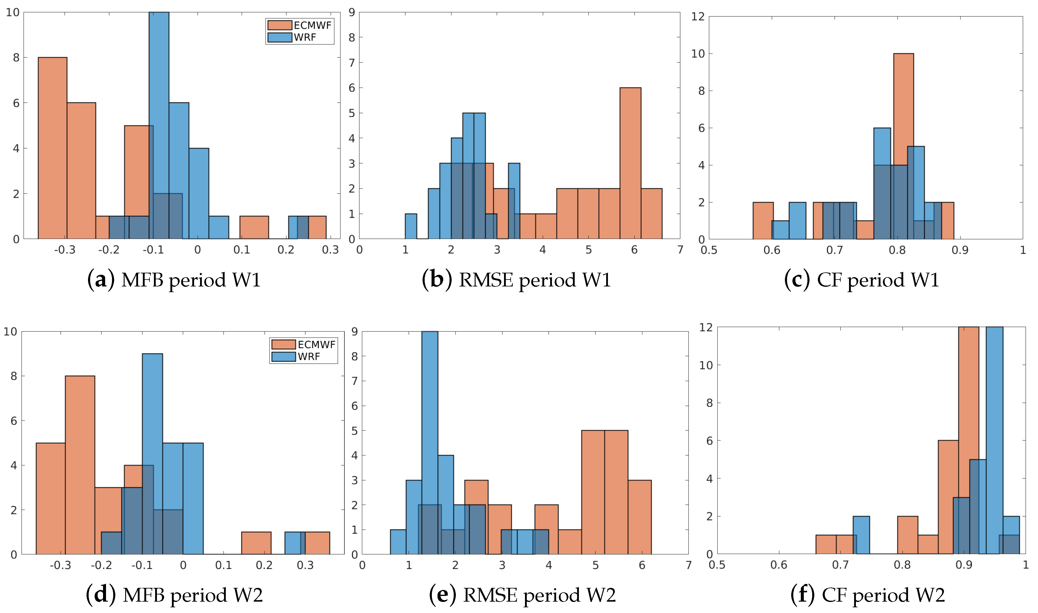
2.4. Statistical Performance Metrics

Three metrics were computed to compare the simulations and evaluate LOTOS–EUROS’s performance using input data from ECMWF and WRF. The evaluation considers diurnal cycles to compare the simulation results and vertical profile for pollutants.
The first is the mean fractional bias (MFB). The MFB normalizes the bias for each model–observation pair dividing by the model and observation average before taking the sample mean:
MFB = 2 M i = 1 M y L E i y i o y L E i + y i o ,
where M is the number of elements in the set.
In this application, M equals the number of observations from all valid monitoring station data for the period of interest, y i L E is the model simulation output, and y i o is the observation.
The MFB ranges from 2 to + 2 and has the advantage of preventing bias from a few dominating high-value observation–simulation pairs in case of strong variations; for instance, due to a strong diurnal cycle [32].
In contrast, the root-mean-square error (RMSE) calculates the sample standard deviation of the discrepancies between the predicted and observed values (see Equation (3)). The RMSE emphasizes high-variance errors by giving more significant absolute errors greater weight than smaller ones [33]:
RMSE = 1 M i = 1 M y L E i y i o 2 .
The last metric is the correlation coefficient (Corr), which shows how the values from one dataset (simulations) relate to the value of a second dataset (observations). A high value (approaching +1.0) is a strong direct relationship. Values near 0.5 are classed as moderate relationships, and values below 0.3 show weak relationships. A low negative value (approaching −1.0) is a strong inverse relationship, and values near 0.0 indicate a small, if any, relationship. The correlation coefficient is calculated following [34]:
Corr = i = 1 M ( y L E ) i ( y L E ) ¯ ( y i o y o ¯ ) i = 1 M ( y L E ) i ( y L E ) ¯ 2 i = 1 M ( y i o y o ¯ ) 2 .
where overline denotes a sample mean over M elements of the validation set.

2.5. Ground-Based Sensor Network for Validation

SIATA (Sistema de Alerta Temprana del Valle de Aburrá) is a metropolitan sensor network that monitors air quality and meteorology variables using multi-parametric sensors in the Aburrá Valley metropolitan area. The network is distributed across the five most populated municipalities in the valley, with a concentration of sensors in Medellín, the lower part of the valley. The project began as a thesis by Luz Jeannette Mejia in 1999, focusing on rain monitoring using 20 manual pluviometry sensors through the SIMPAD program, the precursor to the DAGRD. In 2004, the Mayor of Medellin and the Metropolitan area joined the project, recognizing it as a metropolitan initiative. The Universidad EAFIT now executes the project.
The air quality network studies O 3 , SO 2 , PM 10 , PM 2.5 and PM 1 measurements. To validate the results of this work after the coupling of the WRF with the LOTOS–EUROS, we looked at PM 2.5 . The PM 2.5 equipment consists of Met One Instruments BAM-1020 and BAM-1022 monitors using a beta ray attenuation method to measure airborne PM concentrations [35]. The distribution of stations across the Aburrá Valley is shown in Figure 2a).
The meteorology network of SIATA comprises several types of sensors, including pluviometry level, meteorological, real-time, and infrared cameras, disdrometers, accelerographs, soil monitoring, electric field monitoring, pyranometer networks, and remote sensors such as the hydro-meteorological radar, radiometer, ceilometer network, and vertical wind profiler. Figure 2b) displays the stations used for validation in this study. Only stations that provided at least 85% of the data were considered for analysis. As in a similar experimental setup by [14], wind measurements with speeds below 0.5 m/s were removed. The variables were temporally resampled to a coarser resolution of 1 h to match the temporal resolution of the LOTOS–EUROS and WRF.
Data from the SIATA network were obtained through the SIATA data web portal (data available upon request). The web portal provides graphic visual information from the network stations, meteorological radar data, different forecast methods, satellite information such as NASA’s Global Geostationary weather satellite, geospatial information, and camera networks, among other helpful information. The ground-based data can be accessed through this API by visiting the following link: https://siata.gov.co/siata_nuevo/index.php/mapa, accessed on 9 April 2023. Additionally, the data from the SIATA’s stations can be downloaded by visiting the following link: http://siata.gov.co:8018/descarga_siata/index.php/index2/, accessed on 9 April 2023.

3. Results and Discussion

This section will thoroughly examine and discuss the simulation outcomes using the LOTOS–EUROS model with meteorological data obtained from WRF and ECMWF for two different periods, W1 and W2. By comparing the results of the two periods, we can evaluate the model’s ability to capture the variability of atmospheric pollutant concentrations under different meteorological conditions. Additionally, we may evaluate the representation of the meteorological variables for each model compared to the conditions in the area.

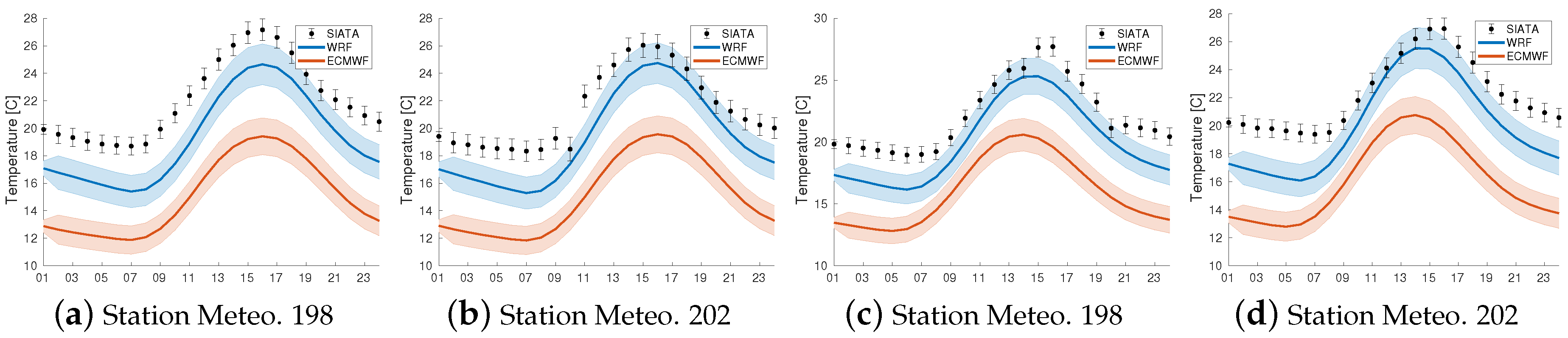
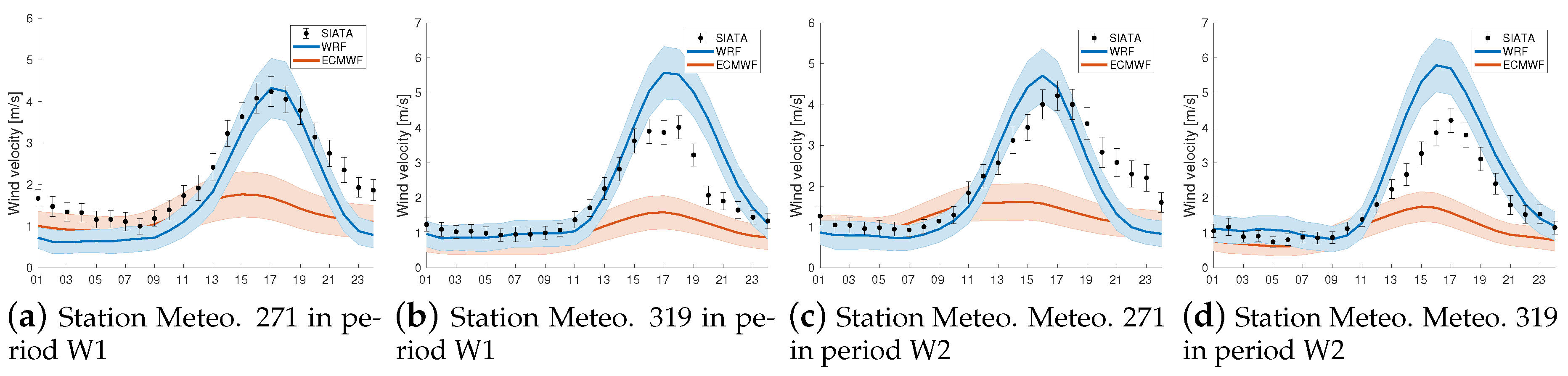
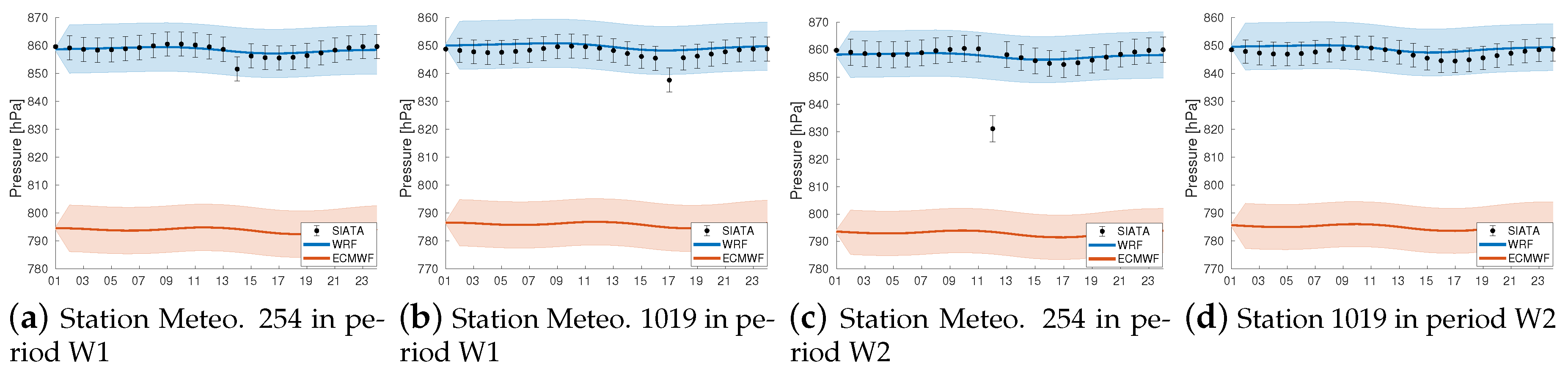
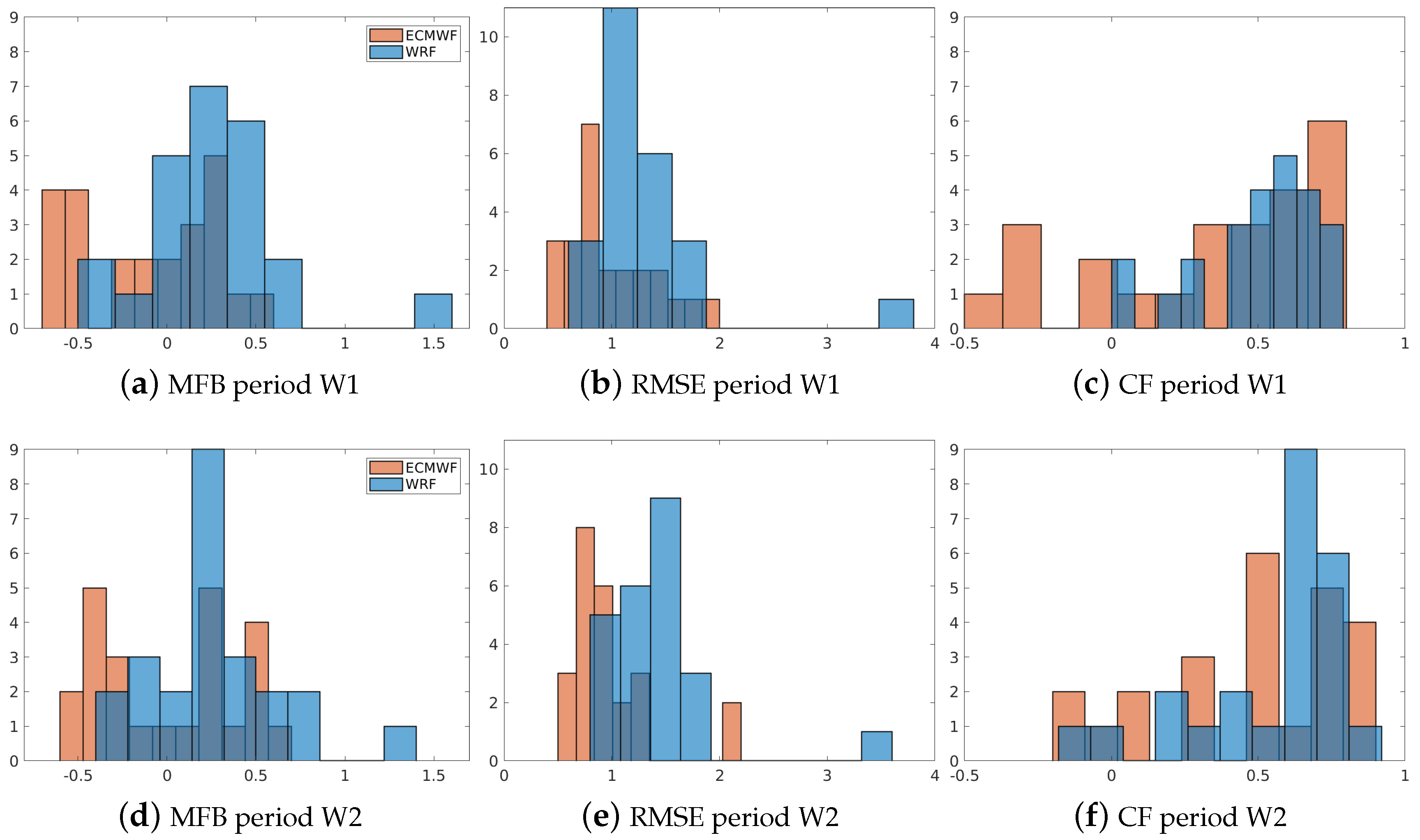
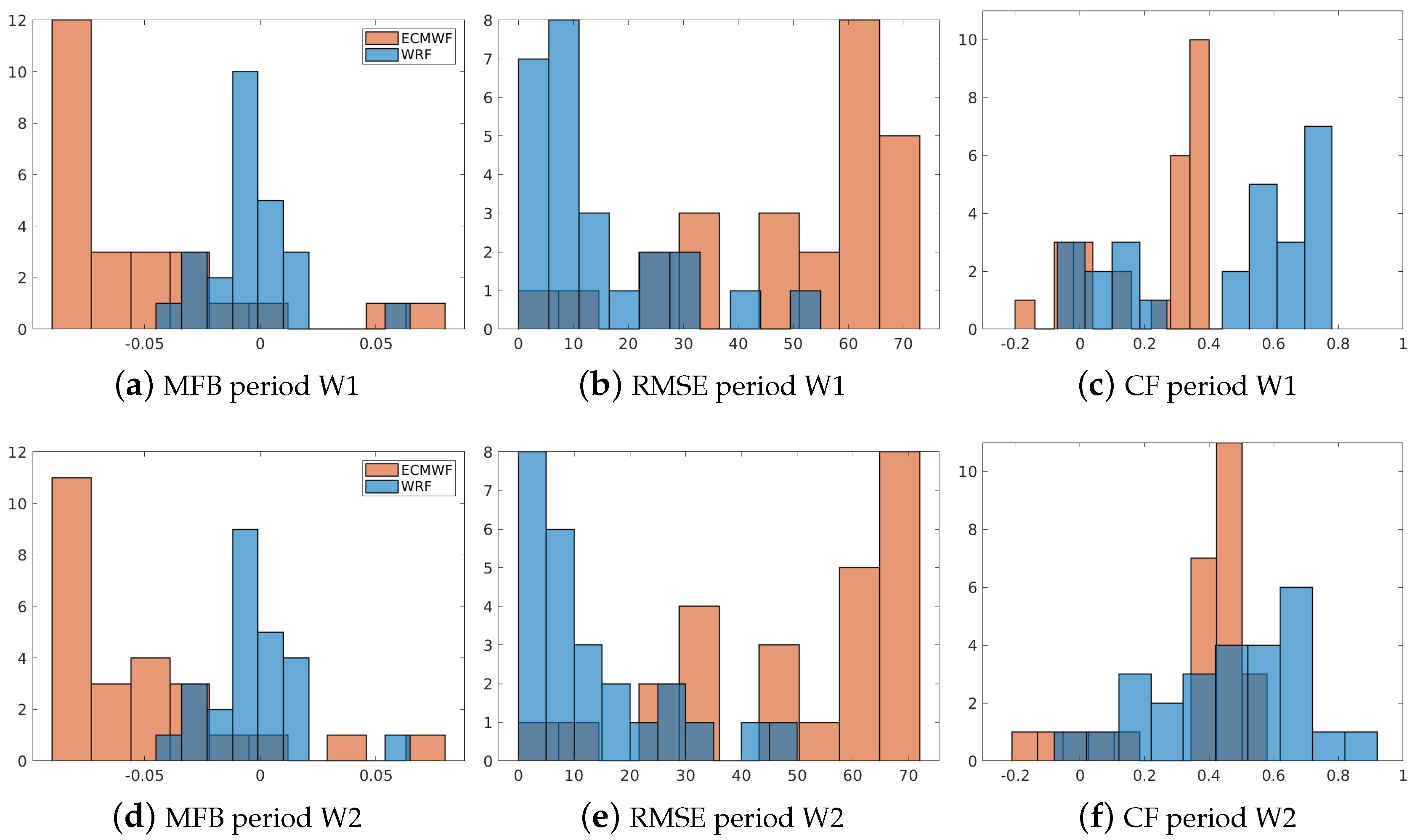
3.1. Comparison of ECMWF and WRF Meteorology

Here, we study the difference between the meteorologies from WRF and ECMWF that serve as input of the CTM LTOS-EUROS. With this, we exhibit the representation that every model offers as the input to the CTM. Wind velocity at 10 m, surface temperature, and surface pressure were the selected variables (see Figure 3).
Figure 3a,d compare the average wind velocity at 10 m. The wind pattern seems smoother for the WRF condition than the ECMWF.
Figure 3b,e correspond to the average surface temperature in the inner domain that contains the Aburrá Valley. It is easy to find here that the WRF meteorology has a better representation of reality, with higher temperatures inside the urban areas inside the valley where the cities are located.
Figure 3c,f represent the average pressure field. Although the ECMWF in Figure 3c tries to represent the valley with an increase in the respective area and the Cauca Valley region, left of the metropolitan area, the WRF is more representative of the natural conditions.
The observed changes in Figure 3 can be primarily attributed to the higher resolution of the WRF meteorology compared to the ECMWF. In addition, WRF is a non-hydrostatic model, which allows for a more accurate representation of the complex vertical and horizontal movements in the mountainous and narrow Aburrá Valley.
Figure 4 displays time-series plots for the daily cycle of surface temperatures (Figure 4a), wind velocity at 10 m (Figure 4b), and surface pressure (Figure 4c) for stations 202, 271, and 1019, respectively. Observe that both models underestimate the surface temperature. However, the underestimation in the ECMWF model is more significant.
Moreover, Figure 4b notes that both models capture the diurnal variation in the wind velocity. However, WRF performs better, showing less variability and closer agreement with the observations. Furthermore, Figure 4b illustrates how the WRF model closely tracks the observed pattern.
Moreover, as illustrated in Figure 4c, both models exhibit a similar daily cycle for surface pressure. However, it can be observed that the WRF model performs better than the ECMWF model in capturing the variability of the observations.
On the other hand, Figure 5, Figure 6 and Figure 7 represent the daily cycle for surface temperature, wind speed at 10 m, and surface pressure at different locations for the two periods, W1 and W2.
The daily cycle is evident in both models, as shown in Figure 5. However, there is an underestimation in both models for the observations. Notably, the underestimation is more significant in the ECMWF model, consistent with the results presented for both periods, W1 and W2.
Figure 6 demonstrates the accuracy of the WRF model in representing the daily cycle of wind speed at 10 m. However, it is observed that both models underestimate the wind speed for the studied periods W1 and W2.
Similarly, Figure 7 shows the accuracy of the WRF model in representing the surface pressure observations in both periods and for the stations shown. Notable is that the surface pressure is an essential meteorological variable in atmospheric circulation and weather forecasting. Its accurate measurement and representation are essential for studying and understanding atmospheric dynamics and weather phenomena.
Figure 8, Figure 9 and Figure 10 exhibit the comparison of performance metrics on the surface temperature, wind velocity at 10 m, and surface pressure for the periods W1 and W2 and the ECMWF and WRF models.
Figure 8 displays the metrics computed for both evaluation periods, W1 and W2. The results for both periods are similar, with both models presenting an underestimation of the average surface temperature. However, the underestimation is more pronounced in the ECMWF model than in the WRF model. Additionally, the histogram shows that the deviation between the observations and the ECMWF model is more significant than between the data and the WRF model. Notably, the WRF model results show higher accuracy and correlation than the ECMWF model in representing the observed data. This is especially evident in the W2 period.
Similarly to temperature, the metrics for wind speed (Figure 9) show a bigger underestimation by the ECMWF model. Remember that the accurate representation of wind speed is crucial in air quality and atmospheric chemistry modelling. Wind speed affects the dispersion and transport of pollutants and plays a crucial role in mixing atmospheric species. With an accurate representation of wind speed, the transport and mixing of pollutants will be accurately modelled, leading to correct predictions of air quality and atmospheric chemistry. Therefore, an accurate representation of wind speed is essential for modelling the formation and transportation of pollutants and aerosols and their chemical transformations in the atmosphere.
The results in Figure 10 demonstrate a notable underestimation and deviation of surface pressure by the ECMWF model compared to the observations. These findings are consistent with the correlation factor reported in Figure 10b,e. It is important to note that an accurate representation of the surface pressure is crucial for numerical weather prediction and atmospheric modelling as it affects the prediction of weather patterns and atmospheric behaviour. Therefore, the underestimation and deviation observed in ECMWF’s representation of surface pressure should be considered when using the ECMWF’s output for weather forecasting or air quality modelling.

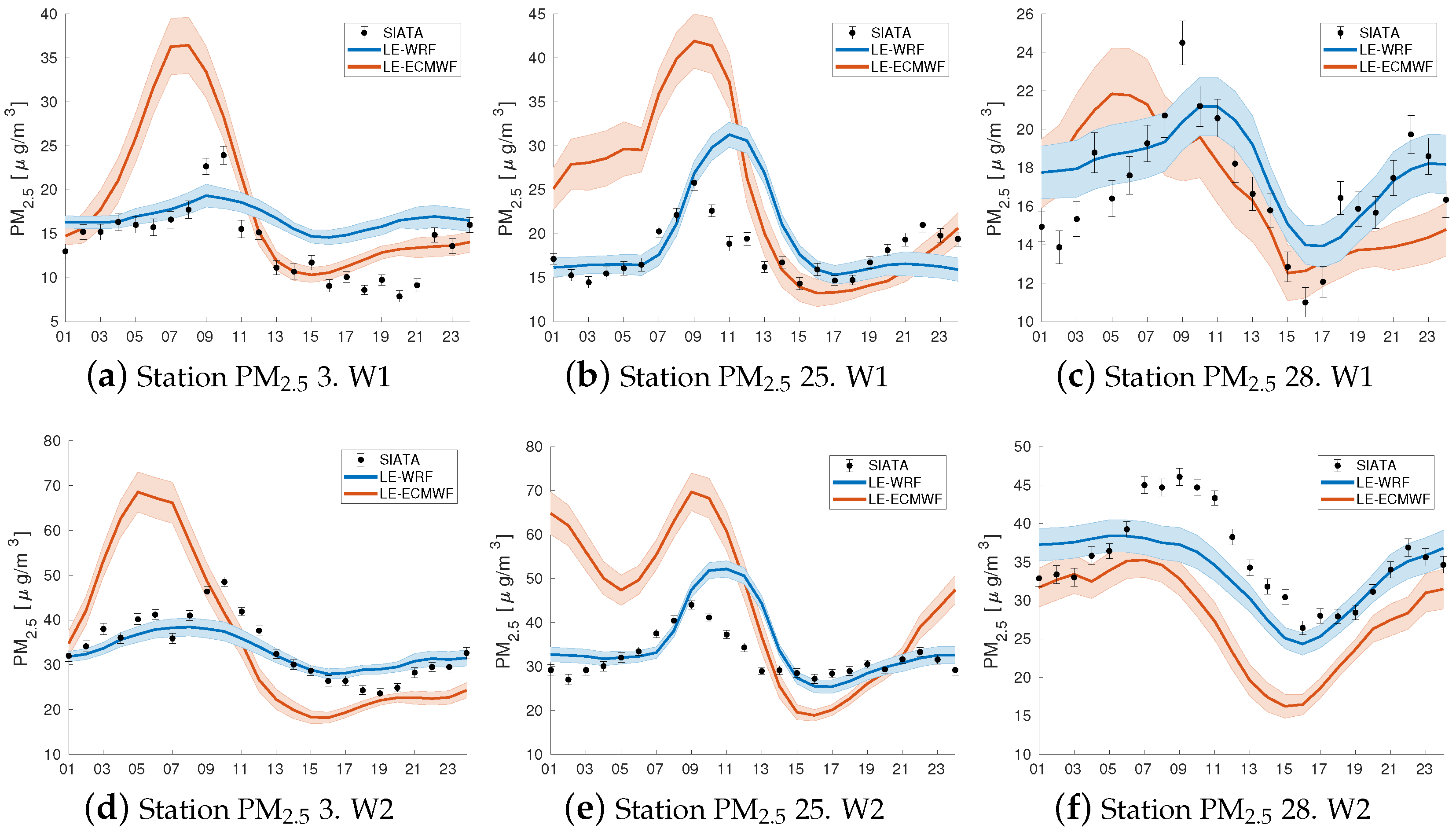
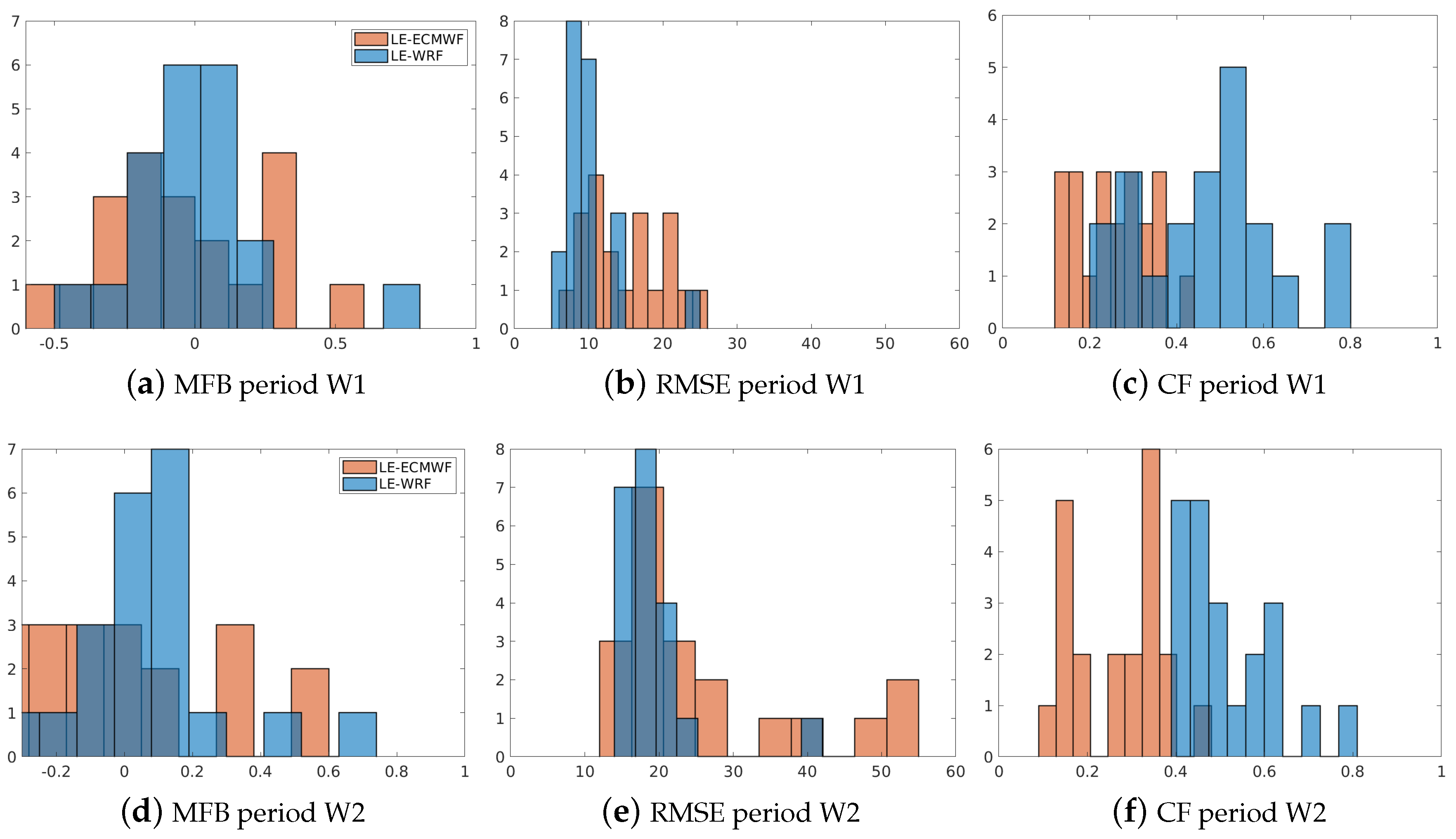
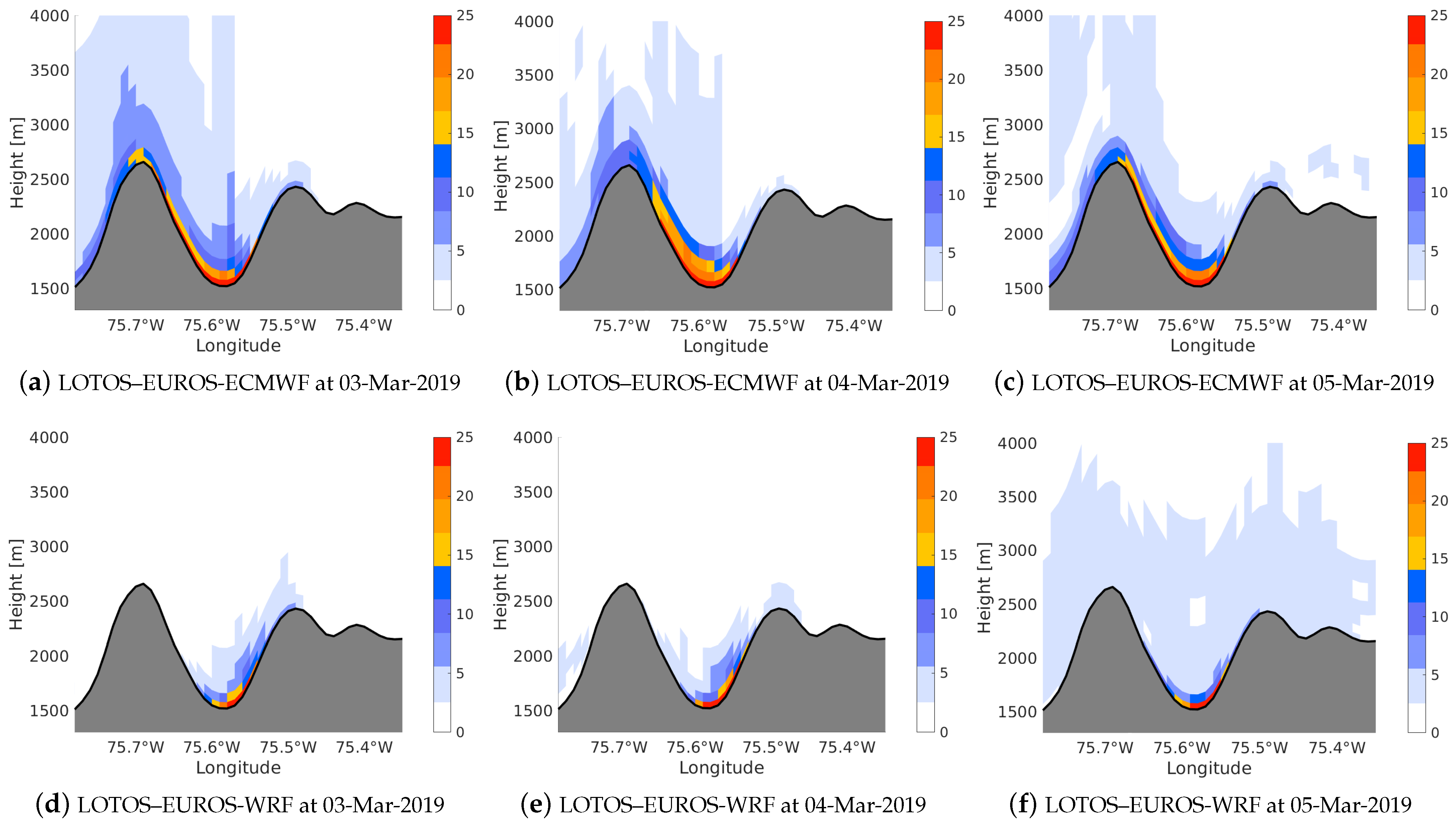
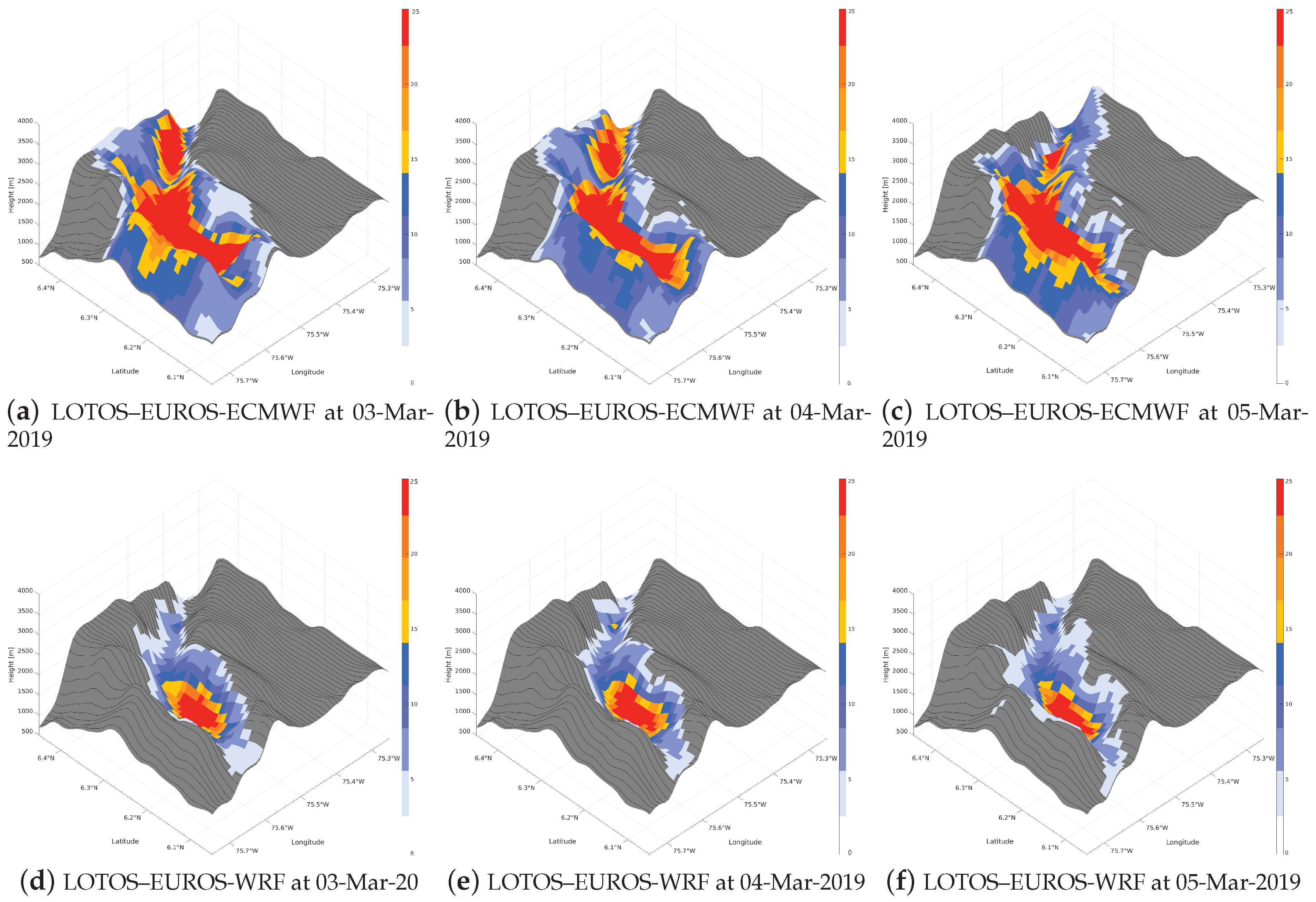
3.2. Comparison of Pollutants Dispersion Patterns of LOTOS–EUROS Model with Both Meteorology

This section aims to evaluate the accuracy and performance of LOTOS–EUROS in representing PM 2.5 with data from ECMWF and WRF. The evaluation includes the representation of the daily cycle and the use of RMSE, MFB, and correlation factor metrics during the W1 and W2 evaluation periods. Furthermore, vertical comparisons are conducted to assess the model’s ability to capture the vertical distribution.
The daily cycle of PM 2.5 by LOTOS–EUROS, using meteorology from WRF and ECMWF, is compared with observations in Figure 11. In this case, Figure 11a–c show the concentration in W1 for stations 3, 25, and 28, respectively. Similarly, Figure 11d–f show the concentration in W2 for the same stations using both ECMWF and WRF meteorology.
The results indicate that the representation of PM 2.5 concentration using ECMWF meteorology tends to overestimate, particularly during the early hours of the day. The results are shown in Figure 11a,b for stations 3 and 25 and both periods, respectively. Furthermore, the figures demonstrate that the concentration variation over time is more significant for the ECMWF results than the WRF.
On the other hand, it is also worth noting in Figure 11 that the WRF’s daily cycle representation by using data from WRF captures the PM 2.5 behaviour in the high-concentration hours. Additionally, both ECMWF and WRF meteorological inputs in LOTOS–EUROS results in a closer representation of the surrounding night hours, with WRF showing a better performance.
Figure 12 shows the error statistics for PM 2.5 obtained from LOTOS–EUROS with ECMWF and WRF meteorological inputs, compared to the observations. The statistics evaluated are RSME, MFB, and correlation factor, and they are presented for the two evaluation periods, W1 and W2.
It is remarkable that the fractional bias in the output for both periods, W1 and W2, is similar, as shown in Figure 12a,d. However, a greater negative bias is observed in W1 (Figure 12a) compared to W2 (Figure 12d).
On the other hand, Figure 12b,e show that, on average, the deviations of the observations are smaller for WRF than ECMWF. Furthermore, the RMSE is more grouped for WRF around a value than in the ECMWF; this is, it is more consistent with the results generated.
As shown in Figure 12c,f, the correlation factor is consistently higher for the results obtained with WRF as input data. Therefore, the WRF model provides better meteorological inputs, resulting in a more accurate PM 2.5 concentration representation in the LOTOS–EUROS model.
The vertical and surface PM 2.5 daily means for the W2 period obtained from LOTOS–EUROS using data from the ECMWF and WRF models are compared in Figure 13. The vertical profiles are presented at the latitude of 6.255° N.
The figures comparing the vertical and surface PM 2.5 concentrations obtained from the ECMWF and WRF models in Figure 13 reveal interesting findings in relation to the input used in LOTOS–EUROS. Specifically, Figure 13a–c demonstrate that the ECMWF model shows high concentrations of PM 2.5 on top of the mountain. In contrast, Figure 13d appears more realistic as it shows PM 2.5 concentrations at the bottom of the valley.
To further analyse the spatial distribution of PM 2.5 in the Aburrá Valley and its representation by LOTOS–EUROS using input from ECMFW or WRF, Figure 14 displays a three-dimensional representation of the average value of PM 2.5 for three days in period W2. The profiles presented correspond to a latitude of 6.255° N.
Based on the analysis of PM 2.5 spatial distributions in the Aburrá Valley using LOTOS–EUROS with the ECMWF and WRF inputs shown in Figure 13 and Figure 14, it is essential to note that there is a significant difference in the representation obtained by the two models. Specifically, the results obtained using ECMWF (Figure 14a–c) show high concentrations on the top of hills and out of the valley, where there is low emission; whereas the results obtained using WRF (Figure 14d–f) show a higher concentration at the bottom of the valley where more of the emissions from industries and population are located. This difference highlights the importance of choosing an appropriate meteorological model input for air quality modelling in different regions.
Previous studies in areas such as the Aburrá Valley have shown that, despite data assimilation, LOTOS–EUROS still has problems in its predictive capacity for PM 10 and PM 2.5 concentrations. One of the possible causes of this uncertainty is the lack of precision in the model inputs, such as emissions inventories and the quality of meteorological information [36].
The default meteorology supplied to LOTOS–EUROS comes from ECMWF [6]. However, previous research has shown that ECMWF does not adequately represent certain complex terrain features, such as mountains and narrow valleys [18], leading to limitations in the accuracy of the representations made by LOTOS–EUROS. Another aspect that made us consider using meteorology inputs that can be custom generated for this region at any time, such as the open-source WRF model, is important as Colombia is not a European Union country limiting its access to the ECMWF dataset.
The WRF model is widely recognized for accurately representing weather and meteorology in regions with complex terrains [18,37,38], such as the Aburrá Valley. In addition, the WRF model can produce local-scale simulations with sub-kilometre resolutions [14] that meet the user’s needs and conditions of the region of interest. On the other hand, unlike ECMWF, the WRF model is non-hydrostatic [39], which allows it to represent vertical movements. Considering these factors, WRF seems to be the natural choice for the studied region.
While using meteorology generated by WRF in LOTOS–EUROS may appear logical, it is crucial to test this hypothesis and demonstrate possible improvements in a scenario such as the Aburrá Valley, which is a narrow valley and experiences poor air quality events throughout the year.
The results presented in this section demonstrate that when WRF generates the meteorology, LOTOS–EUROS improves its representation of the meteorological variables compared to using the meteorology generated by ECMWF. In particular, it is observed that for important meteorological variables, such as atmospheric pressure and winds, the model is closer to the observations and more accurately represents the daily cycles (see Figure 4, Figure 5, Figure 6, Figure 7, Figure 8, Figure 9 and Figure 10). Thus, the accurate representation of daily cycles of meteorological variables, such as surface temperature, wind speeds, and surface pressure, is essential for predicting the dispersion of pollutants in the atmosphere, understanding climate change, and forecasting weather patterns and air mass transportation. These findings emphasize the importance of accurately representing these variables in atmospheric models. This improvement is evident in both periods evaluated, W1 (period of normal concentrations) and W2 (period of high concentrations).
Additionally, the study reveals that the representation of particulate matter by LOTOS–EUROS significantly improves when using WRF meteorological information (see Figure 12). This results in a more accurate spatial distribution of pollutants in the Aburrá Valley (see Figure 13 and Figure 14). Accurate representation of pollutants is vital for CTMs, such as LOTOS–EUROS, to effectively predict the atmospheric dispersion and transportation of pollutants. Inaccurate representation of particulate matter can lead to incorrect air quality predictions, which can lead to erroneous decision-making strategies.

4. Conclusions

The present study compared the CTM LOTOS–EUROS model using meteorology from ECMWF and WRF for two periods (W1 and W2). It work constitutes the first of its nature for the Aburrá Valley—a narrow valley with significant complexity in the terrain.
The results of this study highlight the impact of meteorological inputs on the accuracy of CTM simulations. Furthermore, the study reveals that incorporating WRF-generated meteorological data in the LOTOS–EUROS model improves the accuracy of meteorological variables and its correlation with the observed data within the Aburrá Valley compared with the ECMWF data.
The findings suggest that using WRF input data in the LOTOS–EUROS model improves the PM 2.5 predictions, distribution, and accumulation in the Aburrá Valley. Therefore, using WRF input data is an opportunity for improving the LOTOS–EUROS performance.
We focused the investigation on showing that improving meteorology can lead to a better performance of the CTM model. A future study may include improving the WRF model performance by changing the model’s parameterization through a sensitivity analysis, including more vertical layers, and providing a more accurate representation of the dynamics in the Aburrá Valley. Additionally, it is known that models such as WRF reduce the accumulation of errors when periods of simulations are split. Finally, it is also known that the WRF model output is limited by input data, an issue that can be improved using data assimilation.

Author Contributions

Conceptualization, J.E.H.-R., S.L.-R., O.L.Q. and A.M.R.-P.; methodology, S.L.-R., A.Y.B., O.L.Q., A.S., A.M.R.-P.; software, J.E.H.-R., S.L.-R. and A.M.R.-P.; writing—original draft preparation, J.E.H.-R., S.L.-R. and A.Y.B.; writing—review and editing, J.E.H.-R., S.L.-R., A.Y.B., O.L.Q. and A.H.; data curation, S.I.-C.; funding acquisition, J.E.H.-R. and O.L.Q. All authors have read and agreed to the published version of the manuscript.

Funding

This research was funded by the Universidad EAFIT project called “Sensitivity and Uncertainty of NWP Models”, The Colombian Ministry of Sciences and Technology MINCIENCIAS under the BECAS BICENTENARIO SCHOLARSHIP granted to the main author, and The APC was funded by TU Delft University.

Institutional Review Board Statement

Not applicable.

Informed Consent Statement

Not applicable.

Data Availability Statement

The data are available upon request.

Conflicts of Interest

The authors declare no conflict of interest.

References

  1. Montoya, O.L.; Niño-Ruiz, E.D.; Pinel, N. On the mathematical modelling and data assimilation for air pollution assessment in the Tropical Andes. Environ. Sci. Pollut. Res. 2020, 27, 35993–36012. [Google Scholar] [CrossRef] [PubMed]
  2. Mejía, L.H. Caracterización de la Capa límite Atmosférica en el valle de aburrá a partir de la Información de Sensores Remotos y Radiosondeos. Master’s Thesis, Universidad Nacional de Colombia-Sede Medellín, Medellín, Colombia, 2015. Línea de Investigación: Ciencias de la tierra y del espacio-Meteorología. [Google Scholar]
  3. Jiménez, J.F. Altura de la Capa de Mezcla en un área Urbana Montañosa y Tropical. Caso de Estudio: Valle de Aburrá (Colombia). Ph.D. Thesis, Universidad de Antioquia, Medellín, Colombia, 2016. [Google Scholar]
  4. Bedoya, J.; Martãnez, E. Calidad del Aire en el Valle de Aburrã Antioquia-Colombia. Dyna 2009, 76, 7–15. [Google Scholar]
  5. Rendón, A.M.; Salazar, J.F.; Palacio, C.A.; Wirth, V. Temperature Inversion Breakup with Impacts on Air Quality in Urban Valleys Influenced by Topographic Shading. J. Appl. Meteorol. Climatol. 2015, 54, 302–321. [Google Scholar] [CrossRef]
  6. Manders, A.; Kranenburg, R.; Segers, A.; Hendriks, C.; Jacobs, H.; Schaap, M. Use of WRF meteorology in the LOTOS-EUROS chemistry transport model. In Proceedings of the 11th International Conference on Air Quality—Science and Application, Barcelona, Spain, 12–16 March 2018. [Google Scholar]
  7. Escudero, M.; Segers, A.; Kranenburg, R.; Querol, X.; Alastuey, A.; Borge, R.; De La Paz, D.; Gangoiti, G.; Schaap, M. Analysis of summer O3 in the Madrid air basin with the LOTOS-EUROS chemical transport model. Atmos. Chem. Phys. 2019, 19, 14211–14232. [Google Scholar] [CrossRef]
  8. Arasa, R.; Soler, M.R.; Olid, M. Numerical experiments to determine MM5/WRF-CMAQ sensitivity to various PBL and land-surface schemes in north-eastern Spain: Application to a case study in summer 2009. Int. J. Environ. Pollut. 2012, 48, 105–116. [Google Scholar] [CrossRef]
  9. Tuccella, P.; Curci, G.; Visconti, G.; Bessagnet, B.; Menut, L.; Park, R.J. Modeling of gas and aerosol with WRF/Chem over Europe: Evaluation and sensitivity study. J. Geophys. Res. Atmos. 2012, 117, 1–15. [Google Scholar] [CrossRef]
  10. Hu, X.M.; Klein, P.M.; Xue, M. Evaluation of the updated YSU planetary boundary layer scheme within WRF for wind resource and air quality assessments. J. Geophys. Res. Atmos. 2013, 118, 10490–10505. [Google Scholar] [CrossRef]
  11. Žabkar, R.; Koračin, D.; Rakovec, J. A WRF/Chem sensitivity study using ensemble modelling for a high ozone episode in Slovenia and the Northern Adriatic area. Atmos. Environ. 2013, 77, 990–1004. [Google Scholar] [CrossRef]
  12. Srinivas, C.V.; Hari Prasad, K.B.; Naidu, C.V.; Baskaran, R.; Venkatraman, B. Sensitivity Analysis of Atmospheric Dispersion Simulations by FLEXPART to the WRF-Simulated Meteorological Predictions in a Coastal Environment. Pure Appl. Geophys. 2016, 173, 675–700. [Google Scholar] [CrossRef]
  13. Kumar, A.; Jiménez, R.; Belalcázar, L.C.; Rojas, N.Y. Application of WRF-Chem Model to Simulate PM10 Concentration over Bogota. Aerosol Air Qual. Res. 2016, 16, 1206–1221. [Google Scholar] [CrossRef]
  14. Henao, J.J.; Mejía, J.F.; Rendón, A.M.; Salazar, J.F. Sub-kilometer dispersion simulation of a CO tracer for an inter-Andean urban valley. Atmos. Pollut. Res. 2020, 11, 928–945. [Google Scholar] [CrossRef]
  15. Georgiou, G.K.; Christoudias, T.; Proestos, Y.; Kushta, J.; Pikridas, M.; Sciare, J.; Savvides, C.; Lelieveld, J. Evaluation of WRF-Chem model (v3. 9.1. 1) real-time air quality forecasts over the Eastern Mediterranean. Geosci. Model Dev. 2022, 15, 4129–4146. [Google Scholar] [CrossRef]
  16. Lopez-Restrepo, S.; Yarce, A.; Pinel, N.; Quintero, O.L.; Segers, A.; Heemink, A.W. Urban air quality modeling using low-cost sensor network and data assimilation in the aburrá valley, colombia. Atmosphere 2021, 12, 91. [Google Scholar] [CrossRef]
  17. Lopez-Restrepo, S.; Nino-Ruiz, E.D.; Guzman-Reyes, L.G.; Yarce, A.; Quintero, O.L.; Pinel, N.; Segers, A.; Heemink, A.W. An efficient ensemble Kalman Filter implementation via shrinkage covariance matrix estimation: Exploiting prior knowledge. Comput. Geosci. 2021, 25, 985–1003. [Google Scholar] [CrossRef]
  18. Posada-Marín, J.A.; Rendón, A.M.; Salazar, J.F.; Mejía, J.F.; Villegas, J.C. WRF downscaling improves ERA-Interim representation of precipitation around a tropical Andean valley during El Niño: Implications for GCM-scale simulation of precipitation over complex terrain. Clim. Dyn. 2018, 52, 3609–3629. [Google Scholar] [CrossRef]
  19. Reboredo, B.; Arasa, R.; Codina, B. Evaluating Sensitivity to Different Options and Parameterizations of a Coupled Air Quality Modelling System over Bogotá, Colombia. Part I: WRF Model Configuration. Open J. Air Pollut. 2015, 4, 47–64. [Google Scholar] [CrossRef]
  20. Brunner, D.; Savage, N.; Jorba, O.; Eder, B.; Giordano, L.; Badia, A.; Balzarini, A.; Baró, R.; Bianconi, R.; Chemel, C.; et al. Comparative analysis of meteorological performance of coupled chemistry-meteorology models in the context of AQMEII phase 2. Atmos. Environ. 2015, 115, 470–498. [Google Scholar] [CrossRef]
  21. Herrera-Mejía, L.; Hoyos, C.D. Characterization of the atmospheric boundary layer in a narrow tropical valley using remote-sensing and radiosonde observations and the WRF model: The Aburrá Valley case-study. Q. J. R. Meteorol. Soc. 2019, 145, 2641–2665. [Google Scholar] [CrossRef]
  22. Mues, a.; Kuenen, J.; Hendriks, C.; Manders, a.; Segers, a.; Scholz, Y.; Hueglin, C.; Builtjes, P.; Schaap, M. Sensitivity of air pollution simulations with LOTOS-EUROS to the temporal distribution of anthropogenic emissions. Atmos. Chem. Phys. 2014, 14, 939–955. [Google Scholar] [CrossRef]
  23. Manders, A.M.M.; Builtjes, P.J.H.; Curier, L.; Denier Van Der Gon, H.A.C.; Hendriks, C.; Jonkers, S.; Kranenburg, R.; Kuenen, J.J.P.; Segers, A.J.; Timmermans, R.M.A.; et al. Curriculum vitae of the LOTOS–EUROS (v2.0) chemistry transport model. Geosci. Model Dev. 2017, 10, 4145–4173. [Google Scholar] [CrossRef]
  24. Sauter, F.; der Swaluw, E.V.; Manders-groot, A.; Kruit, R.W.; Segers, A.; Eskes, H. TNO Report TNO-060-UT-2012-01451; Technical Report; TNO: Utrecht, The Netherlands, 2012. [Google Scholar]
  25. Van Loon, M.; Builtjes, P.J.H.; Segers, a.J. Data assimilation of ozone in the atmospheric transport chemistry model LOTOS. Environ. Model. Softw. 2000, 15, 603–609. [Google Scholar] [CrossRef]
  26. Cáceres, R. Impacto de la Asimilación Radar en el Pronóstico de Precipitación a Muy Corto Plazo Usando el Modelo WRF. Ph.D. Thesis, Universidad de Barcelona, Barcelona, Spain, 2018. [Google Scholar]
  27. Skamarock, W.; Klemp, J.; Dudhia, J.; Gill, D.; Zhiquan, L.; Berner, J.; Wang, W.; Powers, J.; Duda, M.G.; Barker, D.M.; et al. A Description of the Advanced Research WRF Model Version 4; NCAR Technical Note NCAR/TN-475+STR; NCAR: Boulder, CO, USA, 2019; p. 145. [Google Scholar] [CrossRef]
  28. Jiménez-Sánchez, G.; Markowski, P.M.; Jewtoukoff, V.; Young, G.S.; Stensrud, D.J. The Orinoco Low-Level Jet: An Investigation of Its Characteristics and Evolution Using the WRF Model. J. Geophys. Res. Atmos. 2019, 124, 10696–10711. [Google Scholar] [CrossRef]
  29. Arregocés, H.A.; Rojano, R.; Restrepo, G. Sensitivity analysis of planetary boundary layer schemes using the WRF model in Northern Colombia during 2016 dry season. Dyn. Atmos. Ocean. 2021, 96, 101261. [Google Scholar] [CrossRef]
  30. Danielson, J.; Gesch, D. Global Multi-Resolution Terrain Elevation Data 2010 (GMTED2010); U.S. Geological Survey Open-File Report 2011–1073; U.S. Geological Survey: Reston, VA, USA, 2011; 26p. [CrossRef]
  31. Petrescu, A.M.R.; Abad-Viñas, R.; Janssens-Maenhout, G.; Blujdea, V.N.B.; Grassi, G. Global estimates of carbon stock changes in living forest biomass: EDGARv4.3—Time series from 1990 to 2010. Biogeosciences 2012, 9, 3437–3447. [Google Scholar] [CrossRef]
  32. Boylan, J.W.; Russell, A.G. PM and light extinction model performance metrics, goals, and criteria for three-dimensional air quality models. Atmos. Environ. 2006, 40, 4946–4959, Special issue on Model Evaluation: Evaluation of Urban and Regional Eulerian Air Quality Models. [Google Scholar] [CrossRef]
  33. Chai, T.; Draxler, R.R. Root mean square error (RMSE) or mean absolute error (MAE): Arguments against avoiding RMSE in the literature. Geosci. Model Dev. 2014, 7, 1247–1250. [Google Scholar] [CrossRef]
  34. Yu, S.; Eder, B.; Dennis, R.; Chu, S.H.; Schwartz, S.E. New unbiased symmetric metrics for evaluation of air quality models. Atmos. Sci. Lett. 2006, 7, 26–34. [Google Scholar] [CrossRef]
  35. Hoyos, C.D.; Herrera-Mejía, L.; Roldán-Henao, N.; Isaza, A. Effects of fireworks on particulate matter concentration in a narrow valley: The case of the Medellín metropolitan area. Environ. Monit. Assess. 2019, 192, 6. [Google Scholar] [CrossRef]
  36. Lopez-Restrepo, S.; Yarce, A.; Pinel, N.; Quintero, O.L.; Segers, A.; Heemink, A.W. Forecasting PM10 and PM2.5 in the Aburrá Valley (Medellín, Colombia) via EnKF based data assimilation. Atmos. Environ. 2020, 232, 117507. [Google Scholar] [CrossRef]
  37. Fernández-González, S.; Martín, M.L.; García-Ortega, E.; Merino, A.; Lorenzana, J.; Sánchez, J.L.; Valero, F.; Rodrigo, J.S. Sensitivity analysis of the WRF model: Wind-resource assessment for complex terrain. J. Appl. Meteorol. Climatol. 2018, 57, 733–753. [Google Scholar] [CrossRef]
  38. Wu, C.; Luo, K.; Wang, Q.; Fan, J. Simulated potential wind power sensitivity to the planetary boundary layer parameterizations combined with various topography datasets in the weather research and forecasting model. Energy 2022, 239, 122047. [Google Scholar] [CrossRef]
  39. Skamarock, W.C.; Klemp, J.B.; Dudhi, J.; Gill, D.O.; Barker, D.M.; Duda, M.G.; Huang, X.Y.; Wang, W.; Powers, J.G. A Description of the Advanced Research WRF Version 3; Technical Report; NCAR: Boulder, CO, USA, 2008; p. 113. [Google Scholar] [CrossRef]
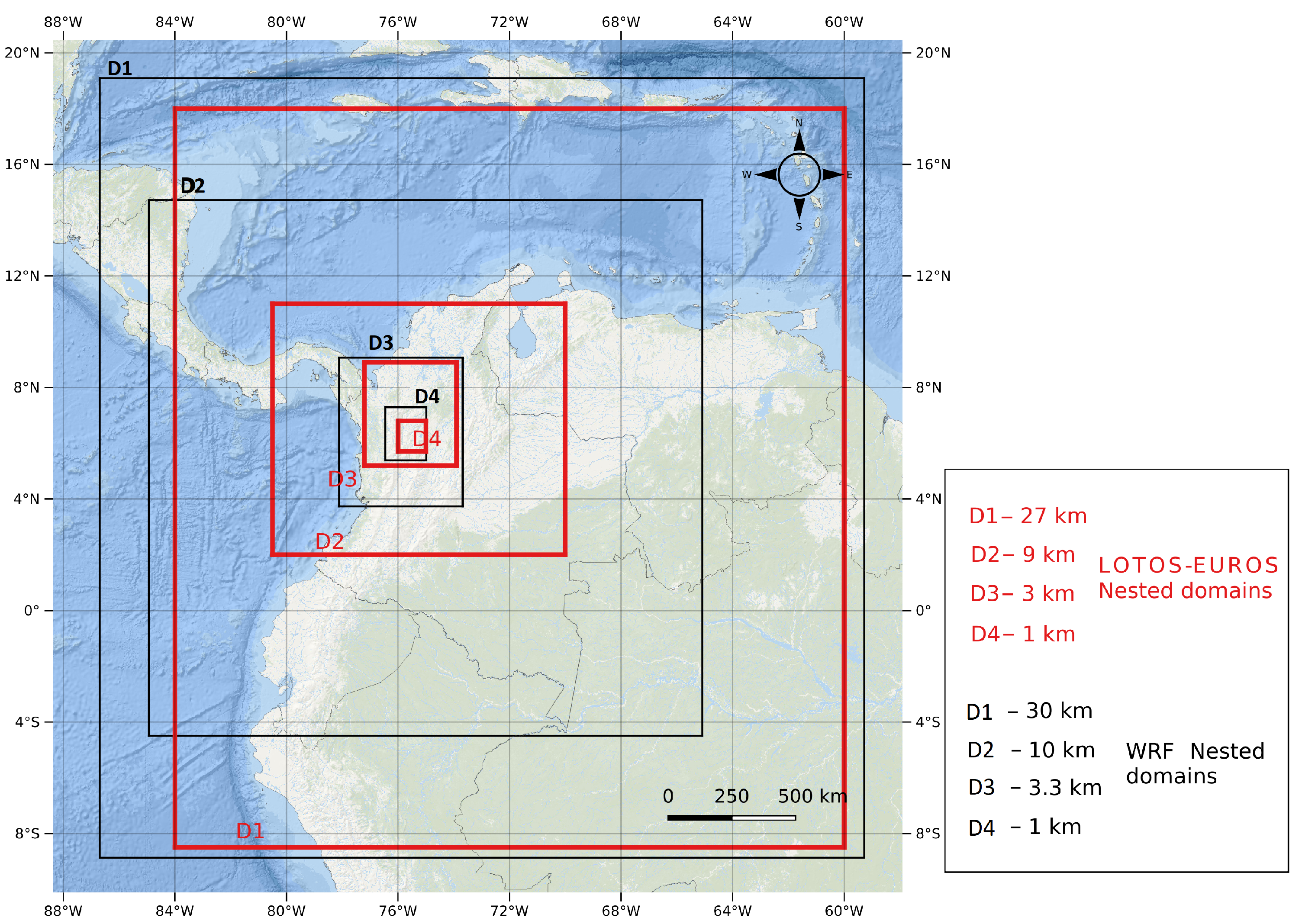
Figure 1. Nested domain configuration of the WRF and the LOTOS–EUROS models for the metropolitan area of the Aburrá Valley. Performance assessment of the LOTOS–EUROS model uses meteorological data obtained from the WRF model and ECMWF.
Atmosphere 14 00738 g001
Figure 2. The locations of the sensors in the Aburrá Valley are shown for (a) the official PM 2.5 monitoring network operated by SIATA and (b) the SIATA meteorological network, which includes sensors for wind, pressure, temperature, and humidity. The spatial distribution of the sensors is essential for accurately measuring and predicting air quality and meteorological conditions in the region.
Atmosphere 14 00738 g002
Figure 3. Comparison of the average surface temperature for ECMWF (a) and WRF (b), the wind velocity at 10 m average for ECMWF (c) and WRF (d), and the surface pressure average field for the ECMWF (e) and WRF (f).
Atmosphere 14 00738 g003
Figure 4. Assessing the performance of the ECMWF and WRF models in predicting temperature at station 202 (a), wind velocity at 10 m (b) at station 271, and surface pressure (c) at station 1019.
Atmosphere 14 00738 g004
Figure 5. Evaluation of daily temperature cycle. Observed data against LOTOS–EUROS simulations with WRF and ECMWF in stations 198 and 202, period W1 (a,b) and period W2 (c,d).
Atmosphere 14 00738 g005
Figure 6. Evaluation of the daily wind velocity cycle. Observed data against LOTOS–EUROS simulations with WRF and ECMWF in stations 271 and 319, period W1 (a,b) and period W2 (c,d).
Atmosphere 14 00738 g006
Figure 7. Evaluation of the daily surface pressure daily. Observed data against LOTOS–EUROS simulations with WRF and ECMWF in stations 254 and 1019, period W1 (a,b) and period W2 (c,d).
Atmosphere 14 00738 g007
Figure 8. Comparison of the surface temperature error statistics between the ECMWF and WRF models for periods W1 and W2. (ac) are MFB, RMSE, and CF in W1, respectively. (df) are MFB, RMSE, and CF in W2, respectively.
Atmosphere 14 00738 g008
Figure 9. Comparison of the wind velocity error statistics between the ECMWF and WRF models for periods W1 and W2. (ac) are MFB, RMSE, and CF in W1, respectively. (df) are MFB, RMSE, and CF in W2, respectively.
Atmosphere 14 00738 g009
Figure 10. Comparison of the surface pressure error statistics between the ECMWF and WRF models for periods W1 and W2. (ac) are MFB, RMSE, and CF in W1, respectively. (df) are MFB, RMSE, and CF in W2, respectively.
Atmosphere 14 00738 g010
Figure 11. Representation of daily cycle of PM 2.5 by LOTOS–EUROS using meteorology from WRF and ECMWF compared with observations. (ac) The concentration in W1 for stations 3, 25, and 28, respectively. (df) The concentration in W2 for stations 3, 25, and 28 ECMWF and WRF, respectively, at different locations.
Atmosphere 14 00738 g011
Figure 12. Comparison of error statistics for PM 2.5 by LOTOS–EUROS employing meteorology from the ECMWF and WRF models for periods W1 and W2. (ac) MFB, RMSE, and CF in W1, respectively. (df) MFB, RMSE, and CF in W2, respectively.
Atmosphere 14 00738 g012
Figure 13. Aburrá Valley vertical profiles. (ac) The vertical and surface PM 2.5 daily mean for a high-concentration period using meteorology from ECMWF in LOTOS–EUROS at latitude 6.255 ° N on 3–5 March. (df) The same for WRF data on the same days.
Atmosphere 14 00738 g013
Figure 14. Comparison of the vertical and surface daily mean PM 2.5 concentrations between the LOTOS–EUROS output using meteorology from the ECMWF and WRF models during three days of a high-concentration period. (ac) The results for 3–5 March 2019, respectively, when using ECMWF input, (df) The results for the same dates when using the WRF input.
Atmosphere 14 00738 g014
Table 1. Distribution of domains in WRF and LOTOS–EUROS.
WRF
DomainLatitudeLongitudeResolution grid
D1−8.86401, 19.0911−86.6947, −59.275330
D2−4.94672, 14.7199−84.929, −65.091610
D33.7342, 9.0649−78.1088, −73.67743.3
D45.3792, 7.2945−76.4586, −74.98141.1
LOTOS–EUROS
DomainLatitudeLongitudeResolution grid
D1−8.5, 18−84, −6027
D22, 11−80.5, −709
D35.2, 8.9−77.2, −73.93
D45.7, 6.8−76, −751
Table 2. Overview of the weather research and forecasting (WRF) model parametrization setup for the experiment.
ProcessScheme
MicrophysicsSingle moment 6-class
Land surfaceThermal diffusion scheme
PBLMYJ
SurfaceMonin–Obukhov (Janjic Eta)
RadiationCAM scheme
Table 3. Overview of the dataset used in the concentration and transport simulations from the LOTOS–EUROS model. The table provides information on the experiment period and types of emissions considered in the simulations, including fire, biogenic, anthropogenic, orography, and land use. Additionally, details are provided on the boundary conditions used in the simulations.
MeteorologyECMWF; D1: 14 km × 14 km, D2, D3, D4: 7 km × 7 km
Initial and boundaryLOTOS–EUROS (D3). Temp.res: 1 h.
conditionsSpat.Res: 3 km × 3 km
Biogenic emissionsMEGAN Spat.res: 10 km × 10 km
Fire emissionsMACC/CAMS GFAS Spat.res: 10 km × 10 km
LanduseGLC2000. Spat.res: 1 km × 1 km
lOrographyGMTED2010. Spat.res: 2 km × 2 km
Disclaimer/Publisher’s Note: The statements, opinions and data contained in all publications are solely those of the individual author(s) and contributor(s) and not of MDPI and/or the editor(s). MDPI and/or the editor(s) disclaim responsibility for any injury to people or property resulting from any ideas, methods, instructions or products referred to in the content.

