Impacts of GNSS RO Data on Typhoon Forecasts Using Global FV3GFS with GSI 4DEnVar

Abstract

The FORMOSAT-7/COSMIC-2 satellites were launched in 2019, which can provide considerably larger amounts of radio occultation (RO) observations than the FORMOSAT-3/COSMIC satellites. The radio signals emitted from the global navigation satellites system (GNSS) are received by these low Earth orbit (LEO) satellites to provide the so-called bending angle accounting for bending of the rays after penetrating through the atmosphere. Deeper RO observations can be retrieved from FORMOSAT-7/COSMIC-2 for use in RO data assimilation to improve forecasts of tropical cyclones. This study used the global model FV3GFS with the finest grid resolution of about 25 km to simulate five selected typhoons over the western North Pacific, including Hagibis in 2019, Maysak and Haishen in 2020, and Kompasu and Rai in 2021. For each case, two experiments were conducted with and without assimilating FORMOSAT-7/COSMIC-2 RO bending angle. The RO data were assimilated by the GSI 4DEnVar data assimilation system for a total period of 4 days (with 6 h assimilation window) before the typhoon genesis time, followed by a forecast length of 120 h. The RO data assimilation improved the typhoon track forecasts on average of 42 runs. However, no significantly positive impacts, in general, were found on the typhoon intensity forecasts, except for Maysak. Analyses for Maysak attributed the improved intensity forecast mainly to the improved analyses for wind, temperature, and moisture in the mid-upper troposphere after data assimilation. Consequently, the RO data largely enhanced the evolving intensity of the typhoon at a more consistent movement as explained by the wavenumber-one vorticity budget analysis. On the other hand, a noted improvement on the wind analysis, but still with degraded temperature analysis above the boundary layer, also improved track forecast at some specific times for Hagibis. The predictability of typhoon track and intensity as marginally improved by use of the large RO data remains very challenging to be well explored.

1. Introduction

The western North Pacific (WNP) ocean is the most active cyclogenesis area with dozens of typhoons every year. Taiwan island is located over the western periphery of the WNP, often impacted by nearby typhoons. According to the data record of the Central Weather Bureau (CWB) in Taiwan, about 3-4 typhoons impact Taiwan every year [1], frequently bringing violent winds, heavy rainfall, landslides, or ocean encroachment that may lead to a huge loss of life as well as the economy [2]. To better predict the track, structure, and intensity of various typhoons to reduce their associated impacts is a challenging task.

In recent years, CWB adopted and implemented the NCEP’s new-generation global model finite-volume cube-sphere global forecast system (FV3GFS) as their new operational system. For improving operational forecasts, the use of a global model can avoid the specification of lateral boundary conditions required for a regional model and, thus, may facilitate a longer prediction for regional weather events. Along the line of global model application to tropical cyclone (TC) forecast, Hazelton et al. used FV3GFS to simulate TCs on the WNP and evaluated the model prediction on TC track and intensity [3]. Chen et al. also used FV3GFS to simulate TCs in six oceanic regions where cyclogenesis is active, and investigated the TC forecast sensitivity to different cloud microphysics schemes [4]. Compared with the operational forecasts of global forecast system (GFS) at NCEP, FV3GFS may provide further improvement on both track and intensity forecasts by 96 h, as shown in the above study.

The improvement on weather forecast of global models greatly relies on the analysis of model initial conditions, which is largely benefited by the global coverage of various satellite observations through data assimilation. Among many types of satellite observations, radio occultation (RO) data are one of the reliable measurements via the global constellation with high-orbit global navigation satellites system (GNSS) satellites. Radio rays emitted by GNSS satellites pass through the atmosphere and tend to bend due to different densities of the atmosphere before being received by low-orbit satellites. This produces the so-called “bending angle” that accounts for bending of a ray, otherwise being straight without the influence of the atmosphere. The bending angle is induced, resulting from the density variation along the ray as a function of atmospheric pressure, water vapor, and temperature. Through data assimilation, the RO-retrieved bending angles can, thus, be ingested into the model to improve the initial analyses. The RO data accuracy is very high in the upper troposphere and lower stratosphere (UTLS), and is comparable to radiosonde measurements [5]. The biases of RO-retrieved temperature in UTLS were very low, resulting in a significant improvement of global analysis and forecasts when a large amount of RO bending angle data were assimilated into a global model [6]. Several studies suggested that assimilation of RO data can provide a better initial condition, in particular for moisture in the lower troposphere, and resulted in better forecast performances on typhoon and tropical cyclogenesis [7].

RO measurements can have a wider coverage than traditional observations, with higher density on the ocean, which is beneficial for improving the model analysis for TC via data assimilation. Many studies utilized the FORMOSAT-3/COSMIC (hereafter FORMOSAT-3) RO data assimilation for improving TC forecasts. Chen et al. (2021) used the global model, model prediction across scale (MPAS), with the GSI hybrid data assimilation (3DEnVar) to assimilate the RO data of FORMOSAT-3 in forecast of Typhoon Nepartak (2016). In the DA, 3DEnVar combined both the 3-D variational method (3DVAR) and the ensemble Kalman filter (EnKF) to update the background co-variances. The results showed that with the improved analysis on the temperature and horizontal wind, track prediction was improved after assimilating the RO data [8]. A mesoscale model, weather research and forecasting (WRF), was also used with a hybrid 3DEnVar to assimilate FORMOSAT-7 RO data for typhoon prediction with a noted reduction in track forecast errors [9].

As a follow-on of FORMOSAT-3, FORMOSAT-7/COSMIC-2 (hereafter FORMOSAT-7), launched in 2019, can provide considerably more RO data, because FORMOSAT-7 can receive the GNSS signals from multiple systems. Currently, signals emitted from both global navigation satellite system (GLONASS) and global positioning system (GPS) are processed by FORMOSAT-7 to provide a daily maximum up to 6000 soundings. Schreiner et al. showed that the accuracy of FORMOSAT-7 RO data was very high compared to radiosonde observations [10]. The use of FORMOSAT-7 RO data provided positive impacts on global and regional weather predictions (e.g., [6,9,11,12,13]). The RO data reduced the tropospheric temperature, humidity, and wind analysis errors, resulting in improved track forecasts of Typhoon Haishen (2020) [9]. Ruston and Healy applied 4-dimension variational data assimilation (4DVAR) to assimilate FORMOSAT-7 RO data, and they found that assimilating RO data can improve the temperature and wind of the stratosphere and humidity of the troposphere in tropical regions [11]. Lien et al. also found that global forecasts using the CWB Global Forecast System (CWBGFS) can be improved, especially for tropical regions, when FORMOSAT-7 RO data were assimilated by the model [6].

CWB has prepared the quasi-operational FV3GFS with the GSI DA system that can assimilate RO data for weather forecasts. In this study, we utilized the CWB FV3GFS system to investigate the RO data impact on typhoon forecasts and will provide a first preliminary report of the forecast performances for track and intensity using the updated 3DEnVar (4DEnVar) of GSI DA for recent typhoons in the vicinity of Taiwan. It is our focal point on the RO data impact in this study without resort to other influencing factors [12]. Section 2 gives an introduction to the CWB-FV3GFS model and the GSI DA system with the assimilation design. The assimilation and forecast results are provided in Section 3. Two specific runs with larger positive impacts on typhoon forecasts are further analyzed in Section 4. Finally, the conclusions are given in Section 5.

2. The Model and Methodology

2.1. CWB-FV3GFS Model

The FV3GFS global numerical weather prediction system combines both global model FV3GFS and data assimilation system GSI 4DEnVar. The FV3GFS global model used the FV3 dynamic core developed by the Geophysical Fluid Dynamic Laboratory (GFDL) in USA [14,15,16,17], and was implemented with GFS physical parameterizations at NCEP. The same FV3GFS was utilized with some local refinements at the CWB for operational global forecasts, herein called CWB-FV3GFS.

The grids of FV3 divide the globe into six tiles, and the amount of the grids in each tile is the same. The FV3 dynamic core uses a finite-volume method to calculate the fluid and the physical quantity with a flux form [17]. Because the flux entering and leaving the finite volume must be the same, it satisfies the physical quantity to be conserved. FV3 also applies Arakawa-D staggered grids to interpolate the wind into Arakawa C-grids, which can improve the resolution of wave activities. At the same time, FV3 uses the Arakawa D-grids to calculate the absolute vorticity to improve the rotation-related physical processes. The horizontal discrete method in FV3GFS is the same as [14,16], but it changed the accuracy of spatial average and pressure gradient from second order to fourth order. In vertical coordinate, FV3 uses Lagrangian vertical coordinate [16] to improve the accuracy and stability of the vertical transport.

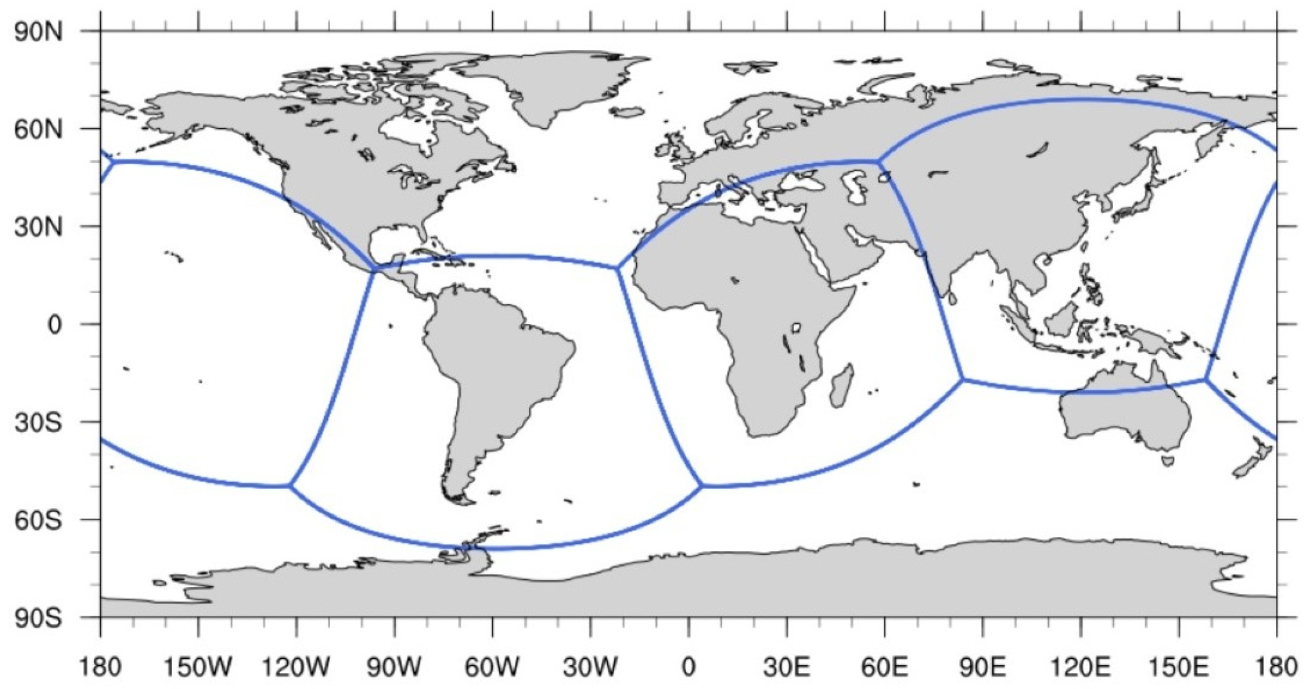
In this study, we used one version of CWB-FV3GFS that was optimally configured with proper physical parameterizations for weather prediction near the Taiwan area. The main deterministic model forecast used a C384T grid (Figure 1), while the short-term ensemble forecasts in the ensemble Kalman filter (EnKF) data assimilation component used a C192T grid. The resolutions of C384T and C192T were about 25 km and 50 km, respectively, where the suffix “T” represents that the grids are configured to put one tile centered in Taiwan. There are 64 vertical layers with the top layer at 1 hPa in the terrain-following coordinate. The GFDL cloud microphysics schemes and cumulus parameterization schemes with scale and aerosol-aware mass-flux shallow and deep convection are used for physical parameterizations in the model.

2.2. GNSS RO Observational Operator

FORMOSAT-7 consisting of six satellites was a cooperative plan between the National Space Organization (NSPO) in Taiwan and NOAA in USA [10,18,19]. FORMOSAT-7 satellites have an orbit of 550 km height and an inclination of 24 degrees, being capable of providing more than 5000 data per day within about 45 degrees of north and south latitudes, about three to four times more than FORMOSAT-3 over the tropical region.

The RO technique is based on Snell’s law that electromagnetic waves entering different media of density would be bent. High-orbit GNSS satellites emit radio waves that are received by the LEO satellites [20]. From the lagging and deflection of the wave signals, observational distance minus geometry straight line distance can be determined as the so-called “excess phase”. Under the hypothesis of spherical symmetry, excess phase can be used to retrieve bending angle and refractivity as well as follow-on products including temperature, pressure, and water vapor profiles for use in DA [21].

The refractivity N related to several atmospheric variables is given by

$$\mathit{N}=\mathbf{77.6}\frac{\mathit{P}}{\mathit{T}}+\mathbf{3.73}\times {\mathbf{10}}^{\mathbf{5}}\frac{{\mathit{P}}_{\mathit{w}}}{{\mathit{T}}^{\mathbf{2}}}$$

(1)

where P, T, and ${\mathit{P}}_{\mathit{w}}$ are dry air pressure, temperature, and water vapor pressure, respectively [22]. It is common to define the refractivity index n by

$$\mathit{N}=\left(\mathit{n}-\mathbf{1}\right)\times {\mathbf{10}}^{\mathbf{6}}$$

(2)

which is related to bending angle through the Abel transform as

$$\mathsf{\alpha }\left(\mathit{a}\right)=-\mathbf{2}\mathit{a}\underset{\mathit{a}}{\overset{\mathit{\infty }}{\int }}\frac{\mathit{d}\mathit{l}\mathit{n}\left(\mathit{n}\right)/\mathit{d}\mathit{x}}{\sqrt{{\mathit{x}}^{\mathbf{2}}-{\mathit{a}}^{\mathbf{2}}}}\mathit{d}\mathit{x}$$

(3)

where $\mathit{a}$ is the impact parameter and x = nr (r the radius to the earth center). For assimilation with RO bending angle, the model related variables are used to obtain the refractivity index and then the bending angle through the Abel transform of (3).

2.3. GSI Hybrid 4DEnVar and Experimental Design

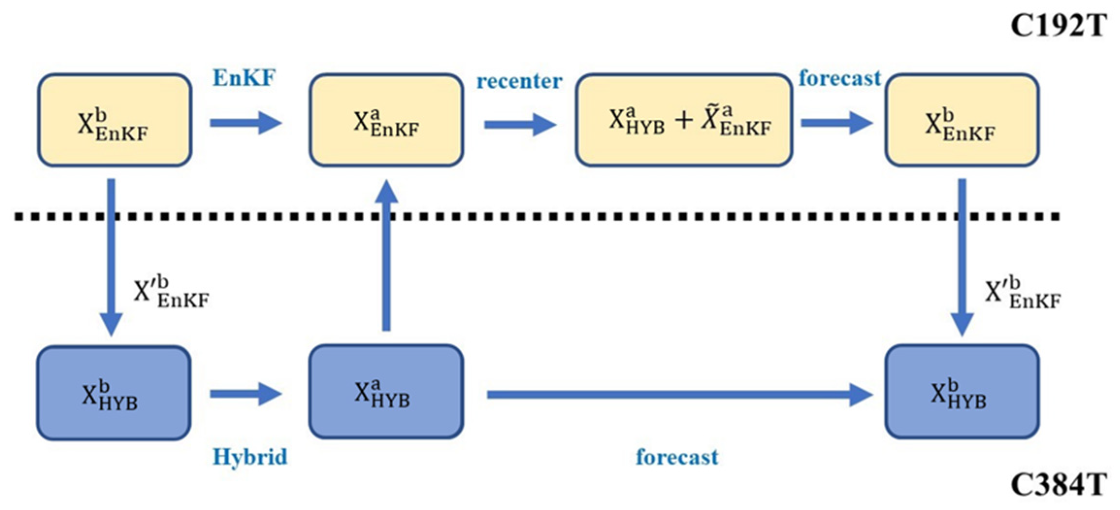
The hybrid four-dimensional ensemble-variational (4DEnVar) data assimilation system developed by NCEP [23,24] was implemented at the CWB. This system is an extension of the hybrid three-dimensional ensemble-variational (3DEnVar) data assimilation [25,26,27,28]. The data assimilation procedure is shown in Figure 2. The use of a coarser resolution for the ensemble forecasts in this study may speed up the DA process. In the 4DEnVar, the temporal evolution of the background error covariance can be approximated by the covariances of ensemble perturbations at discrete times. The background error covariance matrix $\mathbf{B}$ is a weighted average between the static background error covariance in the variational system ${\mathbf{B}}_{\mathbf{V}\mathbf{A}\mathbf{R}}$ and the flow-dependent background error covariance from the EnKF ensemble members ${\mathbf{B}}_{\mathbf{E}\mathbf{n}\mathbf{K}\mathbf{F}}$:

$$\mathbf{B}={\alpha }_1{\mathbf{B}}_{\mathbf{V}\mathbf{A}\mathbf{R}}+{\alpha }_2{\mathbf{B}}_{\mathbf{E}\mathbf{n}\mathbf{K}\mathbf{F}}$$

where ${\alpha }_1$ and ${\alpha }_2$ are their weighting coefficients. In this study, we chose ${\alpha }_1$ and ${\alpha }_2$ to be 12.5% and 87.5%, respectively, for a much larger weight on the flow-dependent background errors. On the other hand, the EnKF analysis members were re-centered to have the mean field same as the hybrid 4DEnVar analysis, while keeping their own perturbation fields. This treatment can avoid the drifting of ensemble members from the deterministic analysis.

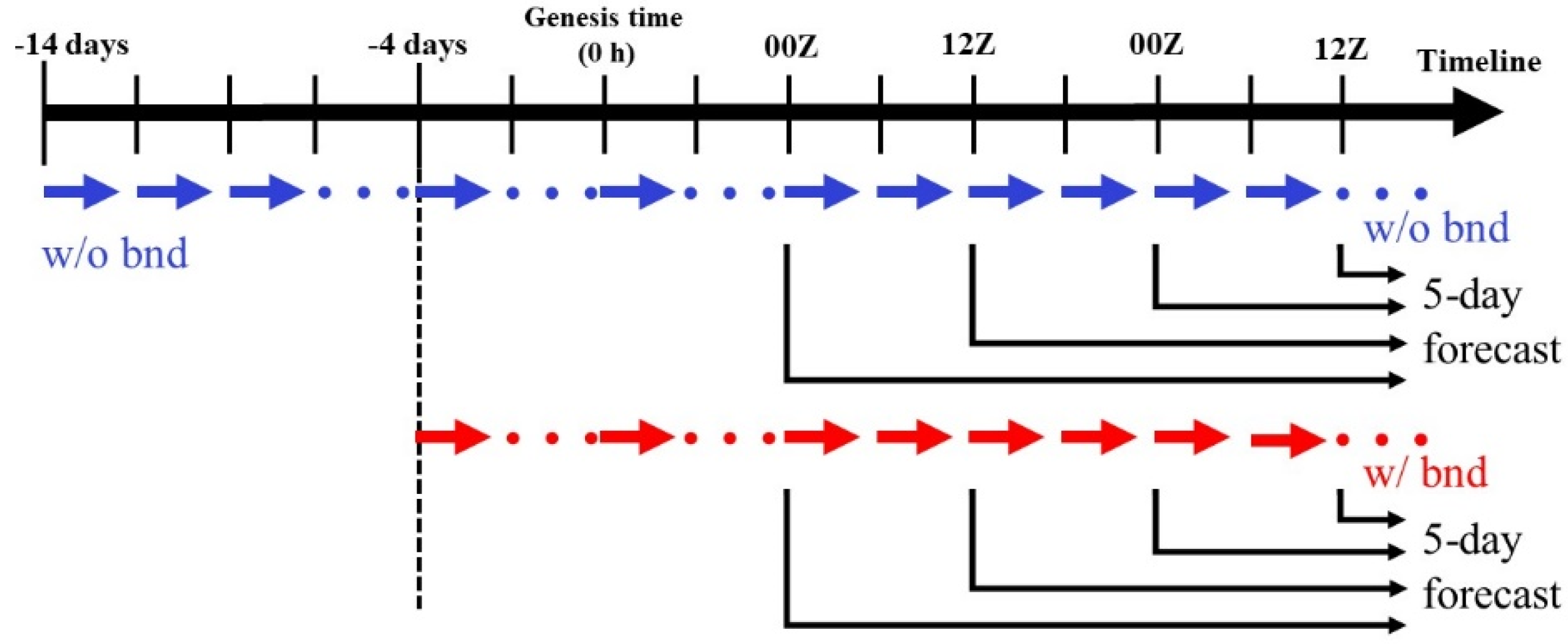
There were 32 ensemble members used in the EnKF system in this study. Figure 3 shows the assimilation strategy and experiment design. For the experiment of each typhoon, ensemble members were initially generated using a stochastic physics method 2 days before the cycled data assimilation started. Considering that the ensemble members randomly generated by this method may not be optimal for the data assimilation, the first 10 days of the continuously cycled data assimilation were reserved as the spin-up period. All available observations operationally used at the CWB except for the FORMOSAT-7 RO data were assimilated 6-hourly here. The assimilated observations, thus, included all real-time satellite data (clear-sky infrared and microwave types) available at NCEP. From the end time of the spin-up, which is just 4 days before the typhoon cyclogenesis, the RO impact experiment (WB), assimilating all available observations plus the FORMOSAT-7 RO data, was initialized and continuously conducted throughout the lifetime of the typhoon. Therefore, the entire experiment needs to be initialized 14 days (10 + 4) before the typhoon cyclogenesis time. This warm start in a shorter period in this study for spinning up the initial ensemble perturbations is a compromised alternative to the perpetual assimilation for operational forecasts at the CWB. At the same time, the original experiment without the FORMOSAT-7 RO data was also continued throughout the same typhoon period, which became the control experiment (NB). About 87% of the total assimilated RO amounts (near 18000 profiles before the typhoon genesis time) were contributed to by FORMOSAT-7. Five-day forecasts initialized at every 00Z, 06Z, 12Z, and 18Z were carried out for both WB and NB (except for some cases only at 00Z and 12Z), followed by a main forecast of 120 h. Note that WB still kept assimilating the RO data after the cyclogenesis of each typhoon.

2.4. Methodology and Typhoon Cases

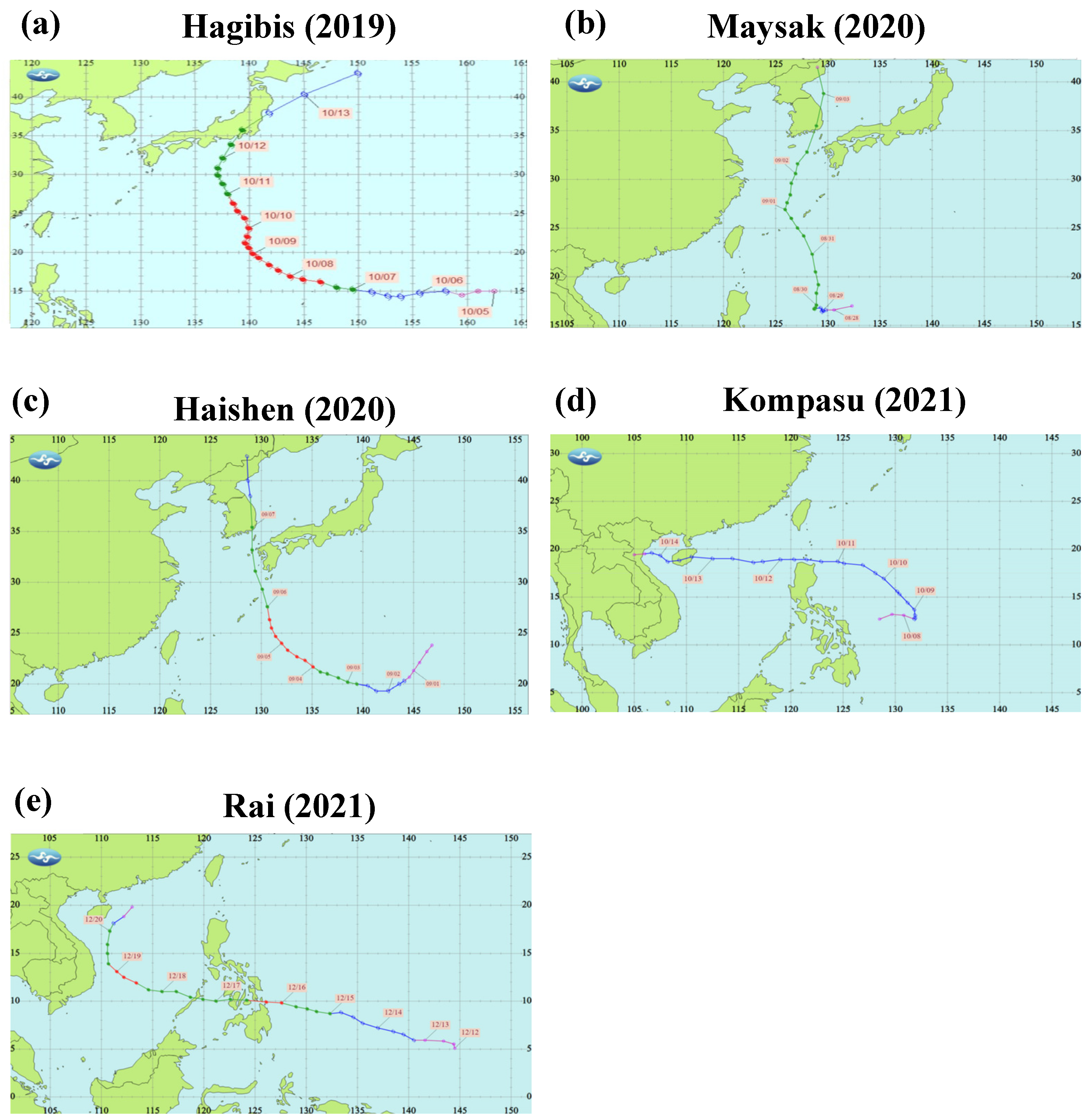
The experiments are conducted for five selected typhoons cases, including Hagibis (2019), Maysak (2020), Haishen (2020), Kompasu (2021), and Rai (2021), as shown in Figure 4. The best tracks provided by CWB were operationally estimated, mostly based on the satellite observations, to detail the paths and stages of the typhoons. There were two daily runs (at 00Z and 12Z) for Hagibis, Maysak, and Haishen, and four runs (at 00Z, 06Z, 12Z, and 18Z) for Kompasu and Rai, Hagibis, Maysak, and Haishen made landfall at Korea or Japan at their later stages; thus, the RO data impact at earlier times can be highlighted without the strong topographical effect involved. Kompasu and Rai made landfall at Philippines at the middle stage, and Rai even became a super typhoon before and after the landfall. Due to the difference in typhoon lifetimes, total forecast runs for each typhoon were different. For the experiments with the CWB-FV3GFS for typhoon forecasts, we will focus on discussing the performances on track and intensity. Results from the DA analysis and forecasts will be analyzed in more detail for two typhoons in comparison with the global analysis as they showed larger positive RO data impacts on track and intensity forecasts. The NCEP global data assimilation system final analysis (GDAS FNL) data were chosen for the comparison in this study, despite the fact that the GDAS assimilation included the RO data.

3. Simulation Results

3.1. Typhoon Tracks

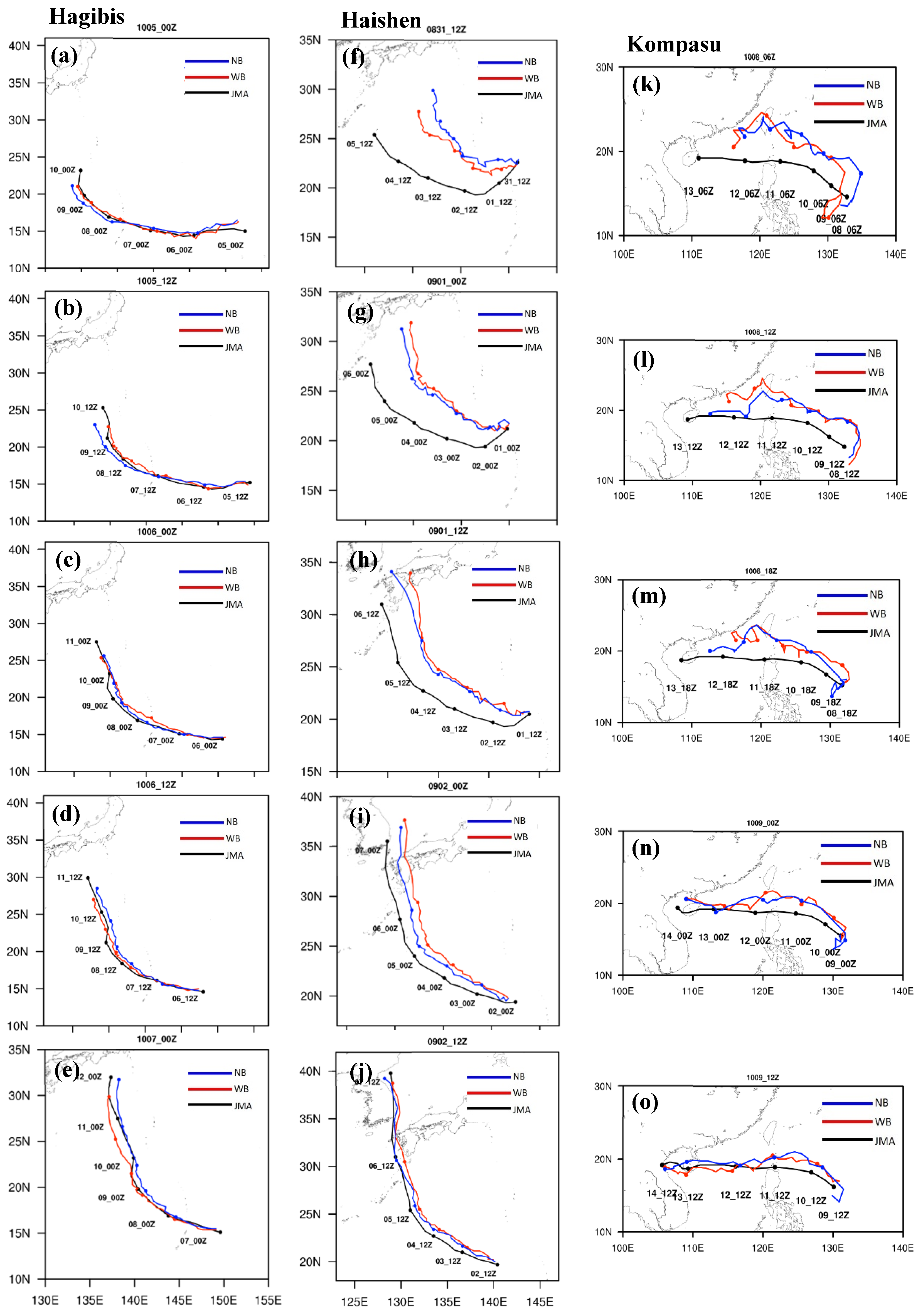
Figure 5 shows the 120 h forecast results of Hagibis, Haishen, and Kompasu. The forecasted tracks for Hagibis at different initial times in general are in good agreement with the Japan Meteorological Agency (JMA)’s best track. In particular, the northward turning of Hagibis at later stages is also well captured with the final track errors less than 200 km (Figure 5c–e). Although Hagibis in WB (with RO data assimilation) forecasts initialized from 0000 UTC and 1200 UTC 5 October 2019 moves slower, its north turn was also well simulated and close to the JMA best track (Figure 5a,b). At the two earlier forecasts, the tracks of NB (without RO data assimilation) were improved in WB, but their performances were mixed for later forecasts. The track forecasts for Haishen and Kompasu, however, showed larger errors from earlier times as compared to Hagibis. Appreciable northward or eastward deviation was produced for Haishen, regardless of use of the RO data (Figure 5f–j). Specifically, the RO data improved the track forecast of the first run (Figure 5f) but degraded the track forecasts of all later runs (Figure 5g–j). The performances of track forecasts are somewhat mixed for Kompasu which is the weakest typhoon (with the maximum wind speed of only 30 m s⁻¹) among the five typhoons. Because of its weak intensity, Kompasu was found to have larger initial position errors than the two other typhoons (Figure 5k–o). Furthermore, Kompasu’s tracks were more meandering than Hagibis and Haishen for both WB and NB. We also did not identify a clearly positive RO impact on the Kompasu’s track forecasts at different initial times, except for the last forecasts that were slightly improved, as seen in Figure 5o.

3.2. Statistics of Forecast Errors

Figure 6a,c,e,h summarize the forecasted tracks of the experiments with and without RO data assimilation at all initial times for the four typhoons (Hagibis, Haishen, Maysak, and Kompasu). There were 6-11 forecasts at each initial time for the four typhoons. For Hagibis, the forecasted tracks exhibited small spreading and follow the best track very well. The track forecasts were slightly degraded by the RO data. The forecasted tracks show larger deviations from the best track for Haishen, with a degradation of the forecasts similar to Hagibis. For Maysak, track deviations were appreciably eastward at the early stage regardless of use of the RO data or not, but largely improved at later stages, especially at 120 h. For Kompasu, the track deviations from the best track were evident at earlier forecasts, but the track forecasts indeed were largely improved at these times. The forecast performances with and without the RO data assimilation were mixed when statistically evaluated by the track errors averaged at different forecast periods for all runs, as shown in Figure 6b,d,f,h. Based on the statistics, we found that the track errors of Hagibis in WB were larger than NB at most of the forecasts, while the track errors for WB were smaller than NB only in the first 24 h and larger than NB at the later times for Haishen. For Maysak, the track errors for WB were smaller than NB at most of the forecast times, especially with a significant reduction of about 50 km at 120 h. For Kompasu, the track errors for both WB and NB were relatively larger, which were considerably reduced (up to 100 km) in WB in first 48 h. This reduction in track errors, however, was not extended to the later forecasts beyond 4 days.

Figure 7 shows the forecast errors of maximum wind speed (V_max) at 10 m height for the four typhoons. We found that all the wind intensity errors at different forecast times were less than 8 m s⁻¹. For the three intense typhoons (Hagibis, Haishen, and Maysak), the forecasted intensities were in good agreement with the best track data in magnitudes and trends (Figure 7a,c,e). For Hagibis, the wind speed error for WB was smaller than NB in the first 24 h, but became larger after 24 h. For Maysak, the V_max forecasts for WB were improved in the first 12 h and 84–108 h, and the largest improvement appears at the later stage. It is also noted that a large improvement of about 2 m s⁻¹ at the earliest stage resulted from the RO data assimilation. For Haishen and Kompasu, the wind speed error for WB was significantly reduced at all the forecast times, except for the 120 h. For these two cases, assimilation of the RO data greatly improved the intensity forecasts.

Figure 8 shows the forecasted minimum sea-level pressure (MSLP) of the typhoon with time for the four typhoons. For the two intense typhoons (Hagibis and Haishen), the deepening rate of MSLP was slower than the JMA best track data in the first three days. For example, near the first occurrence of the lowest pressure of Hagibis (Figure 8a), 1200 UTC 07 October, the forecast gave the MSLP error of about 40 hPa compared with the best track data. Although the forecast obtained the lowest pressure at the later stage, it still had the pressure error of about 10 hPa. For both intense Hagibis and Haishen, the occurrence of the lowest pressure for WB and NB was delayed about two days and one day, respectively, compared with the best track data. The simulated MSLP trends for Hagibis, Haishen, and Maysak were similar, but intense. Hagibis and Haishen were more underpredicted than Maysak prior to the strongest development. The forecasted lowest pressure was about 30 hPa higher than the observed peak intensity at 1200 UTC 4 September for Haishen, but only 15 hPa higher at 0000UTC 1 September for Maysak. For the weaker Typhoon Kompasu, the MSLP errors in the first three days were much smaller than Hagibis, Haishen, and Maysak, but indeed are larger afterward. The lowest MSLP of Kompasu is produced at 0000 UTC 11 October, about two days earlier than the observed at 0000 UTC 13 October. For Hagibis, MSLP errors for WB are smaller than NB in the first 36 h but become larger afterward. On the contrary, MSLP errors for WB are larger than NB in the first 60 h for Haishen and are smaller than NB in 72–96 h and larger than NB at later times. For Maysak, the MSLP errors for WB are considerably smaller than NB at all the forecast times with the largest improvement up to 3–4 hPa. For Kompasu, the MSLP errors in the first 60 h are rather small within 7 hPa, and WB showed some improvement in 72–108 h. Assimilation of the RO data produced fewer positive impacts on intensity forecasts for MSLP, as compared to the intensity forecasts for maximum wind speed (V_max).

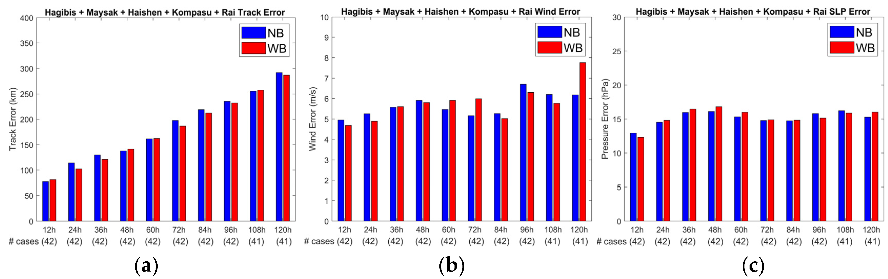
To summarize the impacts of RO data on forecasts of all the typhoons, after including the case of Typhoon Rai, we showed the average track and intensity forecast errors for the five typhoons in Figure 9. Most of the track errors in all the forecasts averaged for the five typhoons were smaller for WB than NB, despite a slight degradation at 48 h and 60 h, based on a total of 42 runs for comparison. The larger improvement of about 20 km on track forecasts was found at both 24 h and 72 h (Figure 9a). For V_max, the performances of WB were somewhat mixed with time. However, we can still identify a noted improvement at 84 h, 96 h, and 108 h (Figure 9b). Note that the forecast errors for V_max are less than about 7 m s⁻¹ in 96 h for both WB and NB. The track forecast errors were slightly larger compared to the typhoon forecasts with a global model in Huang et al. (2022) [29], but the intensity forecast errors for V_max were slightly better than the latter. For MSLP, we found a noted earlier improvement at 12 h in the forecast performance, but then gradually degrading with time as seen in Figure 9c. The degradation was made up by a considerable improvement of about 1 hPa at 96 h. Unlike the track forecasts, the intensity forecast errors did not show a linearly increasing trend with time. On average, the overall forecast results appeared to highlight a larger positive impact on improving the track forecast than the intensity forecast.

4. Case Analysis

To further explore the forecast performances with the RO data assimilation, we choose two cases, the moderate Maysak and intense Hagibis for more detailed analysis. For the first case (Maysak), the RO data assimilation leads to the most pronounced improvement on intensity forecasts. Figure 10 shows the vertical velocity and water vapor at 850 hPa in the NCEP FNL analysis and the forecast results of WB and NB when the simulated Maysak developed at 1200 UTC 30 August 2020. A clear eyewall was present in the FNL analysis with a wide range of upward motions in the spiral bands surrounding the vortex center (Figure 10a). Larger water vapor in the typhoon was produced east of the vortex center (Figure 10b). There were some differences between the FNL analysis and the simulation of WB; for example, upward motions in the eyewall were weaker in WB, but with more water vapor especially at the southeast quadrant (Figure 10c,d). We can find that there were differences between the NB and FNL analyses. First of all, the upward motion of NB was limited in the eyewall region, and the vertical motions north of the Maysak’s center were weak and associated with a less organized rainband (Figure 10e). Secondly, both WB and NB fail to predict the rainband south of the Maysak’s center. Finally, more water vapor was produced to the south and southwest of the typhoon center for NB than WB (Figure 10f).

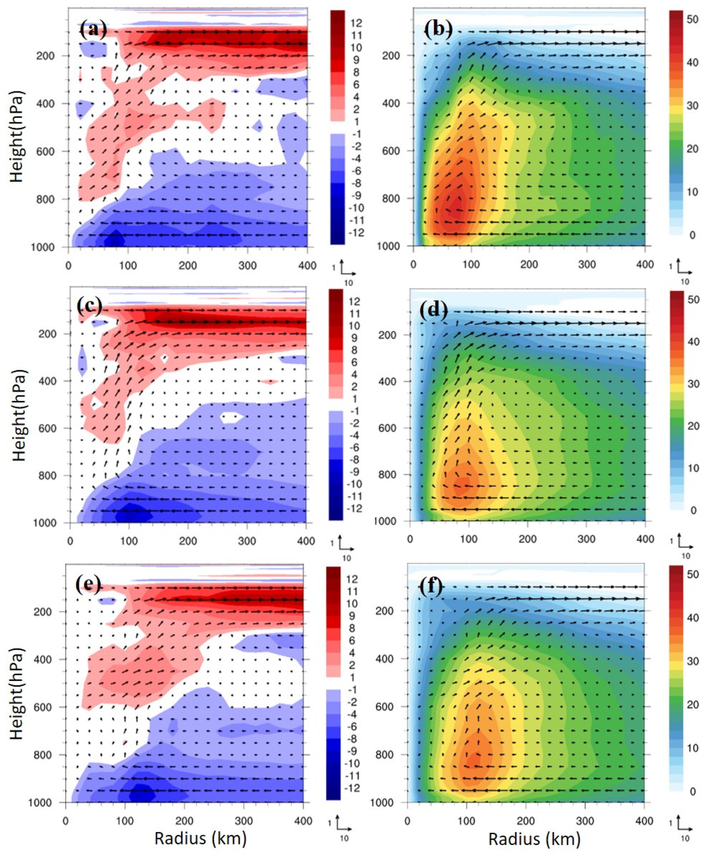
Figure 11 shows the azimuthal-mean fields for Maysak at 1200 UTC 30 August 2020. There is strong inflow at low levels in radii of about 60 to 280 km in the NCEP FNL analysis, with the maximum inflow speed near the radius of 80 km (Figure 11a). The inflow intensified inward and became shallower in the eyewall, which was accompanied by the updraft development tilting outward with height. Near the top of the developed eyewall updrafts, intense outflow over 10 m s⁻¹ was produced outside the radius of 100 km. The associated tangential wind was also strong, close to 50 m s⁻¹ in the lower eyewall region (Figure 11b). For WB, the simulations bore resemblance to the NCEP FNL analysis, except with a weaker inner-vortex core but stronger upper-level eyewall updrafts in a deeper inflow layer (Figure 11c,d). This is consistent with Figure 10 that shows stronger eyewall updrafts in the more intense vortex core at lower levels in the FNL analysis. On the other hand, the simulations for NB (without the RO data assimilation) showed less developed eyewall updrafts that are displayed more outward (Figure 11e,f). The inner-vortex core is also located more outward than the FNL and WB, but with similar intensity as WB. The further outward eyewall updrafts in NB may result from the outer formation of the maximum inflow by about 20 km and 50 km in comparison to WB and FNL, respectively. Overall, the simulations for WB have more consistent features in common with the FNL analysis than NB.

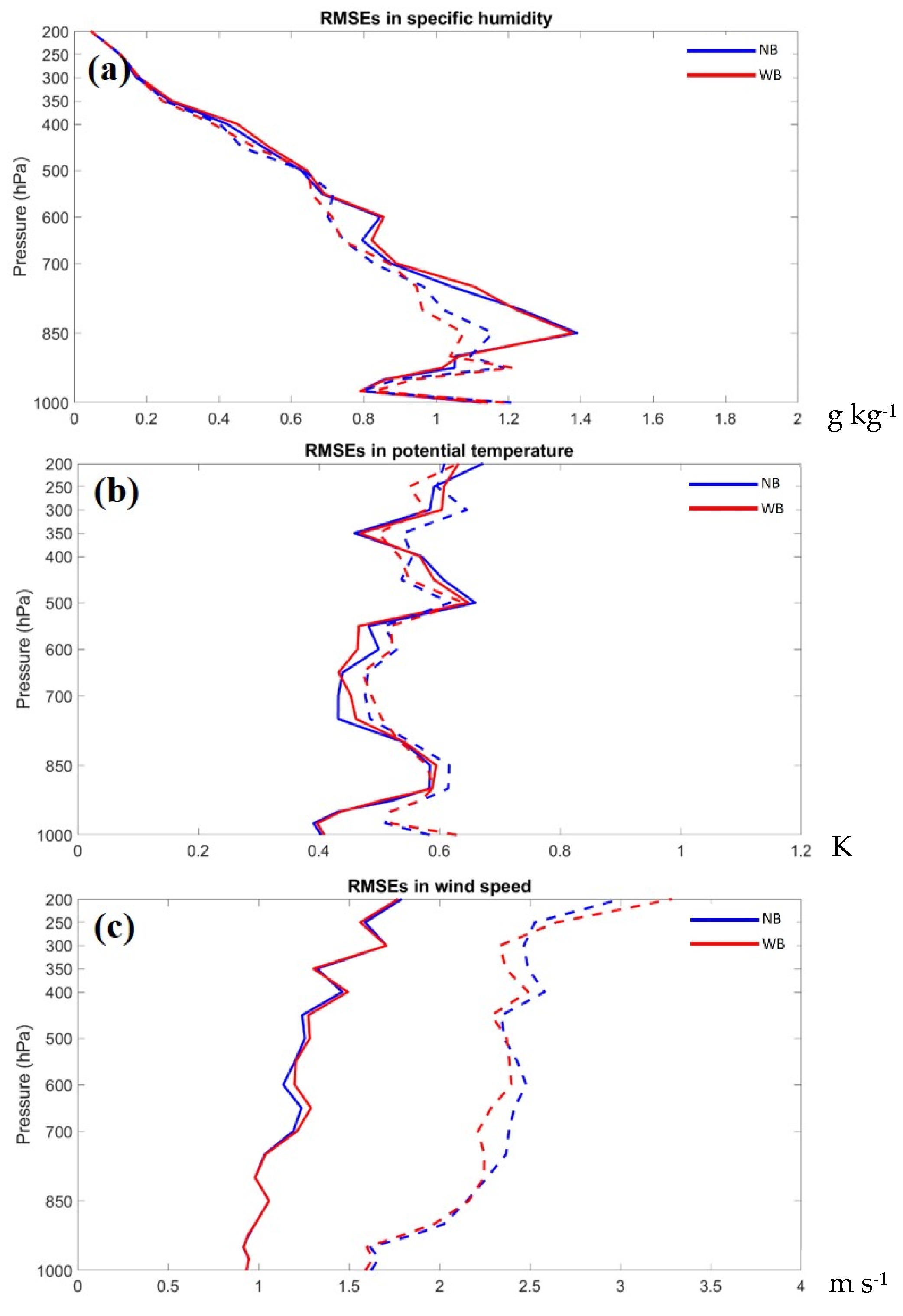
The root mean square errors (RMSEs) were used to evaluate the forecast performances of WB with the RO data assimilation, as shown in Figure 12, for three analysis fields (specific humidity of water vapor, potential temperature, and horizontal-wind speed). The RMSEs against the NCEP FNL were computed for the experiments of WB and NB over the verification region of 20° by 20° centered at the MSLP position of the moving typhoon. We chose the analysis for Maysak at 1800 UTC 24 August and 1200 UTC 30 August 2020, which are the end of DA cycle in the first day and the end of DA cycle after one week, respectively. In general, RMSEs of both WB and NB were systematically larger at the end of the last day than the first day, possibly due to the increased model forecast errors with time, except for the analysis of water vapor in the lower-mid troposphere that was largely improved with smaller RMSEs, especially for WB (Figure 12a). However, such improvement was evident also in NB, indicating that the reduction in RMSEs with time did not completely result from the RO data impact. For potential temperature, the forecast performance of WB after one-week DA cycle is mixed throughout the whole troposphere in comparison to NB (Figure 12b). However, there was a noted improvement near 850 hPa after the last DA cycle. On the other hand, the wind speed analysis was slightly degraded in the mid-troposphere after the first DA cycle for WB, but significantly improved in 300-800 hPa after the completed DA, despite some degradation above 250 hPa (Figure 12c). As seen in Figure 8, the intensity forecasts for Maysak were largely improved throughout the total period of 120 h in WB, which may result from the above improved analyses in the lower-mid troposphere after the DA with the RO data. Consequently, the track forecasts in general were improved in 120 h, although being worse at 48 and 60 h (Figure 6f).

We applied the regression method (Wu and Wang 2000) [30] for the vorticity budget to explain the movement of the simulated vortex for Maysak as employed before [31]. The wavenumber-one vorticity budget terms, averaged in 1–8 km height, for the inner typhoon and the regressed moving speed (m s⁻¹) induced by different physical processes in the budget at 1200 UTC 30 August 2020 are shown in Figure 13. Both vertical vorticity advection and the solenoidal term are much smaller and, thus, are not included in the figure. The induced moving speed of the vortex for WB was slightly slower and less westward than NB (Figure 13a,b), which was in response to their dominant horizontal vorticity advection (Figure 13c,d). The total translation velocity induced by the net budget was in agreement with the wavenumber-one asymmetric flow surrounding the inner vortex. The stretching effect from the divergence term was much weaker than the horizontal vorticity advection, but with counteracting southward and southeastward movement in WB and NB, respectively (Figure 13e,f). This may imply that the vortex movement was much less influenced by the effect of diabatic heating produced by the upward motions of the eyewall due to the horizontal convergence.

The impacts of RO data on the intensity forecast performance for Maysak may be exhibited by the development of absolute vorticity averaging in the radius of 150 km from the vortex center, as shown in Figure 14. The simulated absolute vorticity of Maysak for both WB and NB gradually intensifies with the forecast time, and reaches the peak intensity in 700–850 hPa near 60 h; afterwards, Maysak made landfall in Korea with a significant weakening for both WB and NB (Figure 14a,b). Apparently, WB was stronger in the mid-upper troposphere than NB within the long forecast time up to about 95 h (Figure 14c). However, an intensity reduction was produced below 500 hPa at the early stage by 24 h for WB. As seen in Figure 12, this reduction may be related to the larger RMSEs of potential temperature around 700 hPa for WB. The track of NB by 40 h has a larger westward deviation than WB and the best track of JMA, as shown in Figure 15. This might give a possible link with a short-time weakening in about 25–30 h in Figure 14b. In general, the stronger upper-tropospheric absolute vorticity for WB was consistent with the stronger updrafts in Figure 11.

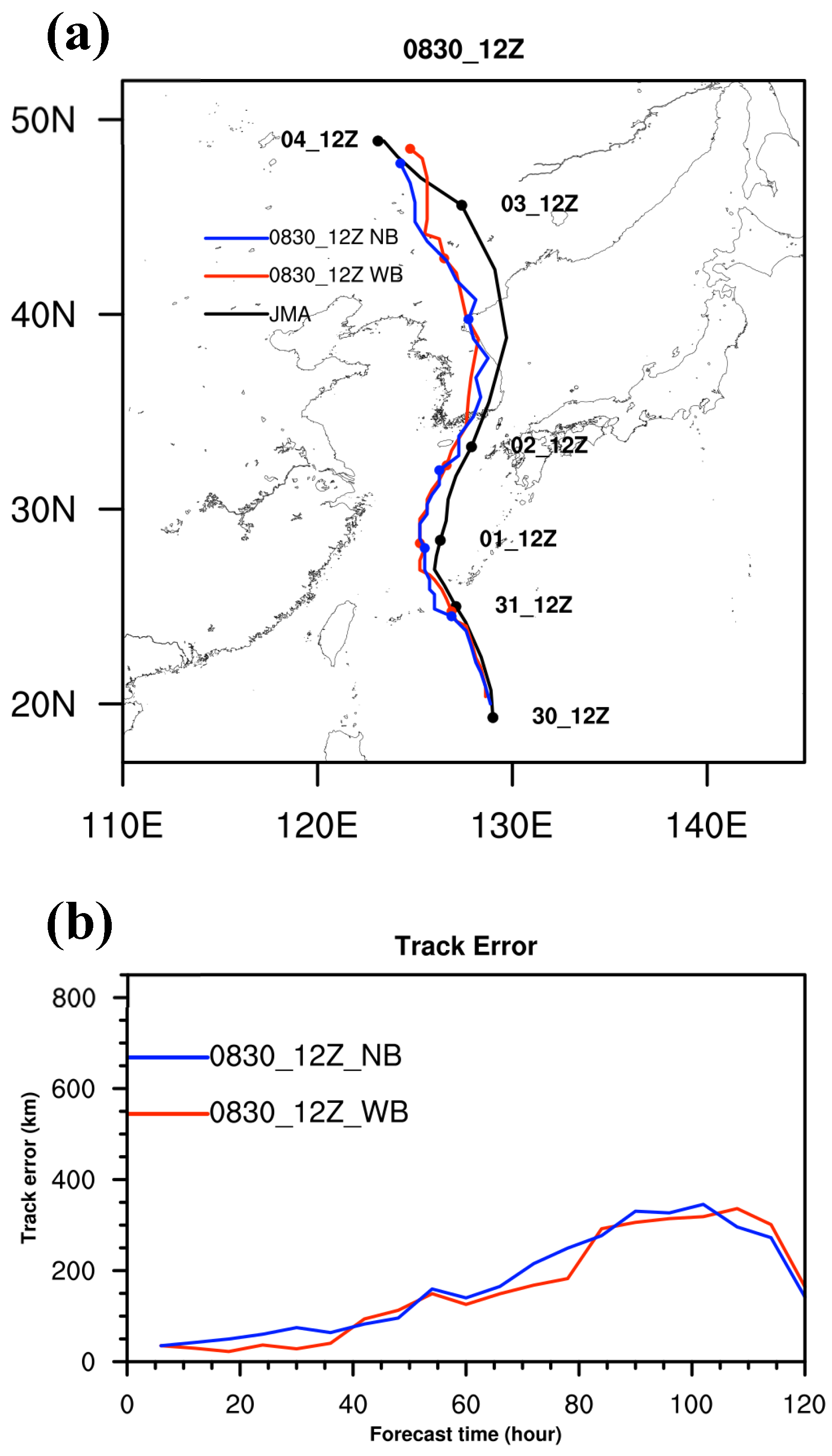
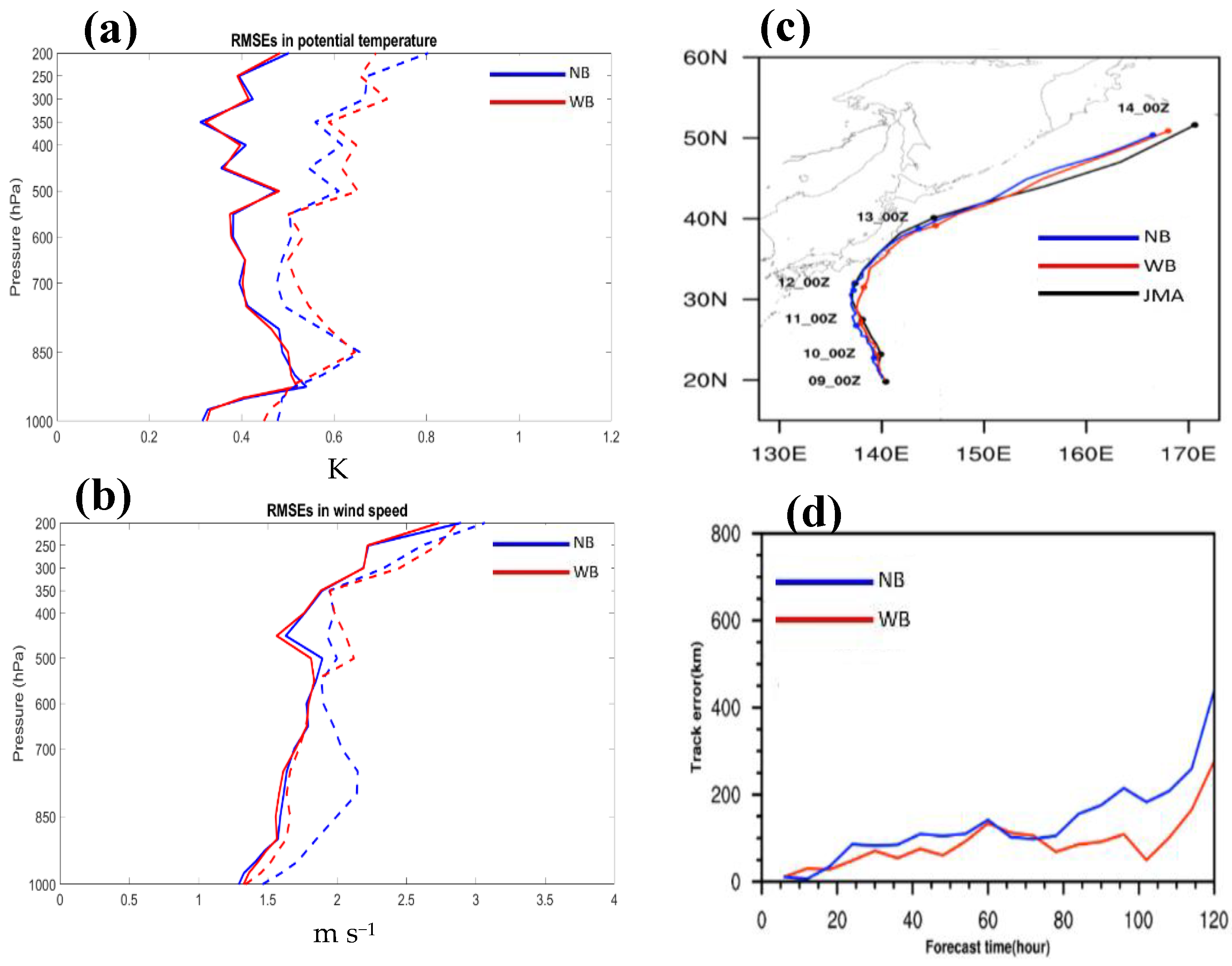
Various analysis results after DA may be produced by the RO data, thus affecting the forecast performances [12]. Herein, we give such an example. Figure 16 shows that the analysis for Typhoon Hagibis was degraded by the additional assimilation of the RO data for potential temperature above 850 hPa, but significantly improved in the wind field below about 550 hPa. The water vapor analysis was relatively less modified by the RO assimilation for this case (figures not shown). This large error reduction in wind analysis led to a considerable reduction in track forecast errors (Figure 16c,d), indicating that the wind analysis is more important for track forecasts in this case. Note that RO data can only contribute to the impacts on wind analysis in DA via dynamic adjustment due to the correlation with thermodynamic variables used in the nonlinear RO operator. This may also outline a difficulty in precisely relating the forecast performances to possible variables involved in the evolution of both track and intensity forecasts.

5. Conclusions

The global model FV3GFS implemented at the CWB was used to investigate the impact of RO data on typhoon forecasts. This study provided a preliminary report of the forecast performance of FV3GFS that made use of the RO data in typhoon forecasts. Five typhoons were selected in this impact study, including Hagibis (2019), Maysak (2020), Haishen (2020), Kompasu (2021), and Rai (2021). The CWB-FV3GFS in combination with the NCEP GSI hybrid 4DEnVar assimilation of RO bending angle, mostly contributed from FORMOSAT-7/COSMIC-2, showed some improvement on the averaged track prediction of about 40 runs for the five typhoons. However, no noticed positive impacts are found on statistical average for the typhoon intensity forecasts of both maximum wind speed and central sea-level pressure, despite non-negligible improvement in some specific runs of the cases. It is particularly noted that the intensity forecasts for Maysak were significantly improved by the RO data.

The assimilation and forecasts were, thus, verified against the NCEP FNL data for Maysak. The results indicate that the additional FORMOSAT-7/COSMIC-2 RO data assimilation improves the intensity forecast of the typhoon vortex, due to the improved analysis on moisture, temperature, and wind fields in the mid-upper troposphere covering the typhoon. For this case, the track forecasts are not improved as greatly as the intensity forecasts, due to the fact that the track errors are still good without the additional FORMOSAT-7/COSMIC-2 RO data assimilation and generally less than 250 km in 120 h forecasts. These RO data largely increase the vorticity intensity of the typhoon at mid-upper levels throughout the forecast. This improved vortex analysis after DA leads to a less westward bias in track resulting from the improved vortex movement that is essentially dominated by horizontal vorticity advection in the wavenumber-one vorticity budget. For the other case, Hagibis, these RO data indeed degrade the temperature analysis above the boundary layer but significantly improve the wind analysis in the troposphere after the DA. Consequently, the track prediction is largely improved, particularly at later stages, owing to the more consistent flow in the vicinity of the vortex. This is quite interesting as reported herein since RO data often gives relatively more contributions to moisture and temperature analyses than to wind analysis. Nevertheless, such noted improvements encouraged the use of RO data in TC forecasts.

Based on the results presented in the current study, we continued to investigate more recent typhoons using the continuously updated analysis of the CWB-FV3GFS instead of an earlier spin-up procedure. However, the preliminary results with these cases have not yet demonstrated further improvement of typhoon track and intensity forecasts. As the GSI assimilation assumed climatologically static observation errors on default for RO data that are not profile dependent, there are spacy rooms for improving the RO data impact. Some recent work for the improvement of the RO data impact focused on the representation of the RO observation errors according to the local spectrum width of RO signals, such as by Zhang et al. (2023) using the global GSI 3DVAR assimilation [32]. This methodology of applying dynamic RO observation errors will rely on the genuine characteristics of each independent RO profile and should enhance the RO data impact. More elaborate experiments are needed to explore the RO data impact on TC forecasts provided with dynamic observation errors in a future study. Finally, we also considered the dynamic vortex initialization [12] for the CWB-FV3GFS in combination with the RO data assimilation for TC forecasts.

References

- Chen, C.-J.; Lee, T.-Y.; Chang, C.-M.; Lee, J.-Y. Assessing typhoon damages to Taiwan in the recent decade: Return period analysis and loss prediction. Nat. Hazards 2018, 91, 759–783. [Google Scholar] [CrossRef]
- Fogarty, E.A.; Elsner, J.B.; Jagger, T.H.; Liu, K.-B.; Louie, K.-S. Louie. Variations in typhoon landfalls over China. Adv. Atmos. Sci. 2006, 23, 665–677. [Google Scholar] [CrossRef]
- Hazelton, A.T.; Harris, L.; Lin, S.-J. Evaluation of tropical cyclone structure forecasts in a high-resolution version of the multiscale GFDL fvGFS model. Weather. Forecast. 2018, 33, 419–442. [Google Scholar] [CrossRef]
- Chen, J.-H.; Lin, S.-J.; Zhou, L.; Chen, X.; Rees, S.; Bender, M.; Morin, M. Evaluation of tropical cyclone forecasts in the next generation global prediction system. Mon. Weather. Rev. 2019, 147, 3409–3428. [Google Scholar] [CrossRef]
- Kuo, Y.-H.; Wee, T.-K.; Sokolovskiy, S.; Rocken, C.; Schreiner, W.; Hunt, D.; Anthes, R. Inversion and error estimation of GPS radio occultation data. J. Meteorol. Soc. Jpn. 2004, 82, 507–531. [Google Scholar] [CrossRef]
- Lien, G.Y.; Lin, C.H.; Huang, Z.M.; Teng, W.H.; Chen, J.H.; Lin, C.C.; Ho, H.H.; Huang, J.Y.; Hong, J.S.; Cheng, C.P. Assimilation impact of early FORMOSAT7/COSMIC-2 GNSS radio occultation data with Taiwan’s CWB Global Forecast System. Mon. Weather. Rev. 2021, 149, 2171–2191. [Google Scholar]
- Harris, L.M.; Lin, S.-J.; Tu, C. High-resolution climate simulations using GFDL HiRAM with a stretched global grid. J. Clim. 2016, 29, 4293–4314. [Google Scholar] [CrossRef]
- Chen, S.-Y.; Shih, C.-P.; Huang, C.-Y. An impact study of GNSS RO data on the prediction of Typhoon Nepartak (2016) using a multiresolution global model with 3D-hybrid data assimilation. Weather. Forecast. 2021, 36, 957–977. [Google Scholar]
- Chen, S.-Y.; Nguyen, T.-C.; Huang, C.-Y. Impact of radio occultation data on the prediction of Typhoon Haishen (2020) with WRFDA hybrid assimilation. Atmosphere 2021, 12, 1397. [Google Scholar] [CrossRef]
- Schreiner, W.S.; Weiss, J.P.; Anthes, R.A.; Braun, J.; Chu, V.; Fong, J.; Hunt, D.; Kuo, Y.-H.; Meehan, T.; Serafino, W.; et al. COSMIC-2 Radio Occultation Constellation: First Results. Geophys. Res. Lett. 2020, 47, e2019GL086841. [Google Scholar] [CrossRef]
- Ruston, B.; Healy, S. Forecast impact of FORMOSAT-7/COSMIC-2 GNSS radio occultation measurements. Atmos. Sci. Lett. 2021, 22, e1019. [Google Scholar] [CrossRef]
- Chien, T.-Y.; Chen, S.-Y.; Huang, C.-Y.; Shih, C.-P.; Schwartz, C.S.; Liu, Z.; Bresch, J.; Lin, J.-Y. Impacts of radio occultation data on typhoon forecasts as explored by the global MPAS-GSI system. Atmosphere 2022, 13, 1353. [Google Scholar] [CrossRef]
- Chen, Y.-J.; Hong, J.-S.; Chen, W.-J. The Impact of Assimilating FORMOSAT-7/COSMIC-2 Radio Occultation Data on Typhoon Prediction using a Regional Model. Atmosphere 2022, 13, 1879. [Google Scholar] [CrossRef]
- Lin, S.J.; Rood, R.B. An explicit flux- form semi-Lagrangian shallow- water model on the sphere. Quart. J. Roy. Meteorol. Soc. 1997, 123, 2477–2498. [Google Scholar] [CrossRef]
- Lin, S.J. A finite-volume integration method for computing pressure gradient force in general vertical coordinates. Quart. J. Roy. Meteorol. Soc. 1997, 123, 1749–1762. [Google Scholar] [CrossRef]
- Lin, S.-J. A “vertically Lagrangian” finite-volume dynamical core for global models. Mon. Weather. Rev. 2004, 132, 2293–2307. [Google Scholar] [CrossRef]
- Lin, S.-J.; Rood, R. Multidimensional flux-form semiLagrangian transport schemes. Mon. Weather. Rev. 1996, 124, 2046–2070. [Google Scholar] [CrossRef]
- Anthes, R.; Schreiner, W. Six new satellites watch the atmosphere over Earth’s Equator. Eos Trans. Amer. Geophys. Union 2019, 100. [Google Scholar] [CrossRef]
- Chu, C.-H.; Huang, C.-Y.; Fong, C.-J.; Chen, S.-Y.; Chen, Y.-H.; Yeh, W.-H.; Kuo, Y.-H. Atmospheric Remote Sensing Using Global Navigation Satellite Systems: From FORMOSAT-3/COSMIC to FORMOSAT-7/COSMIC-2. Terr. Atmos. Oceanic Sci. 2021, 32, 1–13. [Google Scholar] [CrossRef]
- Anthes, R.A. Exploring Earth’s atmosphere with radio occultation: Contributions to weather, climate and space weather. Atmos. Meas. Tech. 2011, 4, 1077–1103. [Google Scholar] [CrossRef]
- Chen, S.-Y.; Kuo, Y.-H.; Huang, C.-Y. The impact of GPS RO data on the prediction of tropical cyclogenesis using a nonlocal observation operator: An initial assessment. Mon. Weather Rev. 2020, 148, 2701–2717. [Google Scholar] [CrossRef]
- Cardinali, C.; Healy, S. Impact of GPS radio occultation measurements in the ECMWF system using adjoint-based diagnostics. Q. J. R. Meteorol. Soc. 2014, 140, 2315–2320. [Google Scholar] [CrossRef]
- Wang, X.; Lei, T. GSI-bsed four-dimensional ensemble–variational (4DEnsVar) data assimilation: Formulation and single-resolution experiments with real data for NCEP Global Forecast System. Mon. Weather. Rev. 2014, 142, 3303–3325. [Google Scholar] [CrossRef]
- Kleist, D.T.; Ide, K. An OSSE-based evaluation of hybrid variational–ensemble data assimilation for the NCEP GFS. Part II: 4DEnVar and hybrid variants. Mon. Weather. Rev. 2015, 143, 452–470. [Google Scholar] [CrossRef]
- Wang, X.; Barker, D.; Snyder, C.; Hamill, T.M. A hybrid ETKF-3DVAR data assimilation scheme for the WRF model. Part I: Observing system simulation experiment. Mon. Weather. Rev. 2008, 136, 5116–5131. [Google Scholar] [CrossRef]
- Wang, X.; Barker, D.; Snyder, C.; Hamill, T.M. A hybrid ETKF-3DVAR data assimilation scheme for the WRF model. Part II: Real observation experiments. Mon. Weather. Rev. 2008, 136, 5132–5147. [Google Scholar] [CrossRef]
- Wang, X.; Parrish, D.; Kleist, D.T.; Whitaker, J.S. GSI 3DVarbased ensemble-variational hybrid data assimilation for NCEP Global Forecast System: Single-resolution experiments. Mon. Weather. Rev. 2013, 141, 4098–4117. [Google Scholar] [CrossRef]
- Hamill, T.M.; Snyder, C. A hybrid ensemble Kalman filter–3D variational analysis scheme. Mon. Weather. Rev. 2000, 128, 2905–2919. [Google Scholar] [CrossRef]
- Huang, C.-Y.; Lin, J.-Y.; Skamarock, W.C.; Chen, S.-Y. Typhoon forecasts with dynamic vortex initialization using an unstructured mesh global model. Mon. Weather. Rev. 2022, 150, 3011–3030. [Google Scholar] [CrossRef]
- Wu, L.; Wang, B. A potential vorticity tendency diagnostic approach for tropical cyclone motion. Mon. Weather. Rev. 2000, 128, 1899–1911. [Google Scholar] [CrossRef]
- Huang, C.-Y.; Juan, T.-C.; Kuo, H.-C.; Chen, J.-H. Track deflection of Typhoon Maria (2018) during a westbound passage offshore of northern Taiwan: Topographic influence. Mon. Weather. Rev. 2020, 148, 4519–4544. [Google Scholar] [CrossRef]
- Zhang, H.; Kuo, Y.-H.; Sokolovskiy, S. Assimilation of radio occultation data using measurement-based observation error specification: Preliminary Results. Mon. Weather. Rev. 2023, 589–601. [Google Scholar] [CrossRef]
Figure 1.
The tile arrangement of CWB-FV3GFS in which the blue lines divide the global grids into six tiles. One tile is centered at Taiwan.
Figure 2.
The data assimilation procedure of 4DEnVar in one assimilation cycle in a dual-resolution approach where the upper part is ensemble Kalman filter with resolution of C192T (about 50 km resolution) and the lower part is the main deterministic forecast with resolution of C384T (about 25 km resolution).
Figure 3.
The assimilation strategy of this study where blue and red arrows indicate data assimilation cycles without and with RO bending angle observations. A period of 4 days before the typhoon genesis time is chosen for starting the RO assimilation. Main forecasts are conducted with a period of 5 days after DA.
Figure 4.
The best tracks of five typhoons from the CWB include (a) Hagibis (2019), (b) Maysak (2020), (c) Haishen (2020), (d) Kompasu (2021), and (e) Rai (2021). The red symbols in the tracks indicate the typhoon stage of the cyclone (plots are available from the CWB).
Figure 5.
The 120 h forecasted tracks with (red) and without (blue) the RO data assimilation for Hagibis (left a–e), Haishen (middle f–i), and Kompasu (right k–o) at different initial times (on top of each panel), overlapped with the best track of JMA (black). The solid dots in the tracks indicate the UTC times at an interval of 24 h.
Figure 6.
(a) The track forecasts with (red) and without (blue) the RO data assimilation of Typhoon Hagibis at different initial times, (b) as in (a) but for average track forecast errors of all runs at each forecast time; (c,d) as in (a,b), respectively, but for Typhoon Haishen; (e,f) as in (a,b), respectively, but for Typhoon Maysak. (g,h) as in (a,b), respectively, but for Typhoon Kompasu. The number of forecast runs at different forecast times are indicated by the numbers in the parentheses below the panels of (b,d,f,h).
Figure 7.
Evolution of the forecasted maximum wind speed at 10 m height with forecast time for the experiments with (red) and without (blue) the RO data assimilation for (a) Hagibis, (c) Hagibis, (e) Maysak, and (g) Kompasu, with the averaged errors of the forecasts at the same forecast time shown in (b, d, f, h), respectively.
Figure 8.
Evolution of the forecasted minimum sea-level pressure of the typhoon
with time for the experiments with (red) and without (blue) the RO data assimilation for (a) Hagibis, (c) Hagibis, (e) Maysak, and (g) Kompasu, with the averaged errors of the forecasts at the same forecast time shown in (b), (d), (f), and (h), respectively.
Figure 9.
(a) Track errors at different forecast times averaged for the five typhoons (Hagibis, Maysak, Haishen, Kompasu, and Rai) for NB (blue) and WB (red), (b) as in (a), but for maximum wind speed errors, and (c) as in (a) but for minimum sea-level pressure errors. The total runs at different forecast times are indicated by the number included in the parentheses below each panel.
Figure 10.
(a) The omega vertical velocity (shaded colors in Pa s−1) at 850 hPa at 1200 UTC 30 August 2020 in the NCEP FNL analysis for Typhoon Maysak, (b) as in (a) but for specific humidity of water vapor (g kg−1). (c) and (d) as in (a) and (b), respectively, but for WB, and (d) and (f) as in (a) and (b), respectively, but for NB. In each panel, horizontal wind velocity (vectors in m s−1) overlaps with a reference vector (50 m s−1) at the lower right.
Figure 11.
Azimuthal-mean fields for Maysak at 1200 UTC 30 August 2020 for (a) the radial-vertical wind of the NCEP FNL data with shaded contours (in m s−1) for radial wind velocity, (b) as in (a) but shaded contours (in m s−1) are for tangential wind velocity, (c) and (d) as in (a) and (b), respectively, but for WB, and (e) and (f) as in (a) and (b), respectively, but for NB.
Figure 12.
RMSEs of (a) specific humidity of water vapor (g kg−1), (b) potential temperature (K), and (c) horizontal-wind speed (m s−1) verified against the NCEP FNL analysis over a 20°-by-20° region centered at the typhoon center at 1800 UTC 24 August 2020 (solid lines) and 1200 UTC 30 August 2020 (dashed lines) for Maysak. The results for NB and WB are shown in blue and red lines, respectively.
Figure 13.
The wavenumber-one vorticity budget terms (shaded colors in 10−9 s−2) averaged 1-8 km height and the regressed moving speed (m s−1) induced by different physical processes in the budget at 1200 UTC 30 August 2020 for Maysak. (a) The total (net) budget for WB, (b) as in (a) but for NB. (c) and (d) as in (a) and (b), respectively, but for horizontal advection. (e) and (f) as in (c) and (d) but for horizontal divergence. The wavenumber-one asymmetric flow (black vectors in m s−1) is overlapped in each panel with a reference vector of 10 m s−1 at the upper right. The blue vector (in m s−1) at the vortex center indicates the induced translation velocity of the vortex and its size is indicated at the upper right corner.
Figure 14.
(a) Evolution of absolute vorticity (s −1) averaged in radius of 150 km for Maysak with the forecast hours starting from 1200UTC 30 August 2020 for WB, (b) as in (a), but for NB, and (c) as in (a) but for the difference between WB and NB.
Figure 15.
(a) Tracks of WB (in red) and NB (in blue) and the best track of JMA (in black) starting from 1200UTC 30 August 2020 for Maysak. (b) as in (a), but for the track errors of WB and NB with the forecast time (hour).
Figure 16.
RMSEs of (a) potential temperature (K) and (b) horizontal-wind speed (m s−1) at 0000 UTC 2 October 2019 (solid lines) and 0000 UTC 9 October 2019 (dash lines) for WB (in red) and NB (in blue). (c) Typhoon tracks of WB (in red) and NB (in blue) and the best track of JMA (in black) starting from 0000 UTC 9 October 2019 for Typhoon Hagibis. (d) as in (c), but for the track errors (km) of WB and NB with the forecast time (hour).
Disclaimer/Publisher’s Note: The statements, opinions and data contained in all publications are solely those of the individual author(s) and contributor(s) and not of MDPI and/or the editor(s). MDPI and/or the editor(s) disclaim responsibility for any injury to people or property resulting from any ideas, methods, instructions or products referred to in the content. |
© 2023 by the authors. Licensee MDPI, Basel, Switzerland. This article is an open access article distributed under the terms and conditions of the Creative Commons Attribution (CC BY) license (https://creativecommons.org/licenses/by/4.0/).
Share and Cite
MDPI and ACS Style
Hong, T.-X.; Huang, C.-Y.; Lin, C.-Y.; Lien, G.-Y.; Huang, Z.-M.; Chen, S.-Y. Impacts of GNSS RO Data on Typhoon Forecasts Using Global FV3GFS with GSI 4DEnVar. Atmosphere 2023, 14, 735. https://doi.org/10.3390/atmos14040735
AMA Style
Hong T-X, Huang C-Y, Lin C-Y, Lien G-Y, Huang Z-M, Chen S-Y. Impacts of GNSS RO Data on Typhoon Forecasts Using Global FV3GFS with GSI 4DEnVar. Atmosphere. 2023; 14(4):735. https://doi.org/10.3390/atmos14040735
Chicago/Turabian StyleHong, Tang-Xun, Ching-Yuang Huang, Chen-Yang Lin, Guo-Yuan Lien, Zih-Mao Huang, and Shu-Ya Chen. 2023. "Impacts of GNSS RO Data on Typhoon Forecasts Using Global FV3GFS with GSI 4DEnVar" Atmosphere 14, no. 4: 735. https://doi.org/10.3390/atmos14040735
Note that from the first issue of 2016, this journal uses article numbers instead of page numbers. See further details here.