Characterization and Source Apportionment of PM in Handan—A Case Study during the COVID-19

Abstract

Handan is a typical city affected by regional particulate pollution. In order to investigate particulate matter (PM) characterization, source contributions and health risks for the general populations, we collected PM samples at two sites affected by a pollution event (12–18 May 2020) during the COVID-19 pandemic and analyzed the major components (SNA, OCEC, WSIIs, and metal elements). A PCA-MLR model was used for source apportionment. The carcinogenic and non-carcinogenic risks caused by metal elements in the PM were assessed. The results show that the renewal of old neighborhoods significantly influences local PM, and primarily the PM₁₀; the average contribution to PM₁₀ was 27 μg/m³. The source apportionment has indicated that all other elements came from dust, except Cd, Pb and Zn, and the contribution of the dust source to PM was 60.4%. As PM_2.5 grew to PM₁₀, the PM changed from basic to acidic, resulting in a lower NH₄⁺ concentration in PM₁₀ than PM_2.5. The carcinogenic risk of PM₁₀ was more than 1 × 10⁻⁶ for both children and adults, and the excess mortality caused by the renewal of the community increased by 23%. Authorities should pay more attention to the impact of renewal on air quality. The backward trajectory and PSCF calculations show that both local sources and short-distance transport contribute to PM—local sources for PM₁₀, and short-distance transport in southern Hebei, northern Henan and northern Anhui for PM_2.5, SO₂ and NO₂.

1. Introduction

In recent years, combined particulate matter (PM) and ozone pollution has been detected in the air in Beijing, Tianjin, Hebei, and the surrounding areas [1]. The PM concentration directly affects public physical and psychological health, and the annual economic loss associated with PM_2.5 (aerodynamic diameter of less than 2.5 µm) and PM₁₀ (aerodynamic diameter of less than 10 µm) health hazards in the Beijing–Tianjin–Hebei (BTH) region is 122.4 and CNY 118.34 billion, respectively [2]. The main components of atmospheric PM include organic carbon (OC), elemental carbon (EC), sulfate (SO₄²⁻), nitrate (NO₃⁻), ammonium (NH₄⁺), and metal elements [3], which are hazardous to humans [4]. PM_2.5 and its components, such as polycyclic aromatic hydrocarbon and hexavalent chromium, are carcinogens. Long-term exposure can increase the carcinogenic risk (CR) [5,6]. Particulate aerosols not only affect public health, but also significantly reduce the downward short-wave flux and boundary layer height due to their radiation effect, and even affect surface temperature and relative humidity [7]. In addition to national or provincial monitoring stations, sensors are being used more and more frequently for air pollutant monitoring [8]. These sensors are favored by researchers because of their convenience and low cost. The use of sensors leads to higher spatial precision in monitoring, but the methods of component detection of particulates are still dominated by on-line aerosol mass spectrometry or off-line sampling plus laboratory testing [9,10,11,12]. Satellite remote sensing has also been used in air quality monitoring in recent years, as it can provide long-term observations with the advantages of wide spatial coverage and multi-element synchronous acquisition. For example, moderate-resolution imaging spectral radiometry (MODIS) provides aerosol optical thickness (AOT) data, which has been widely used in the environment and other fields [13]. In addition, microwave limb sounders (MLSs) [14], infrared atmospheric sounding interferometers (IASIs) [15] and total ozone mapping spectrometers (TOMSs) are being more commonly applied [16]. Satellite remote sensing is mainly used for monitoring gas pollutants such as ozone, sulfur dioxide and formaldehyde, and it cannot achieve near-real-time monitoring because of its high altitude. Badr-Eddine Boudriki Semlali [17] developed a software architecture to combines complex event processing with remote sensing data from various satellite sensors to resolve the problems met in processing data in near-real-time. The “Ground–Satellite” method, which combines ground-based observations with satellite remote sensing, can obtain more pollutant characteristics at both temporal and spatial scales [18], and will be widely applied in the future. The prediction of PM concentration can provide sufficient information for environmental policy decision-makers to take control measures. The traditional prediction models include numerical prediction models (CMAQ [19], CHIMERE [20], AERMOD [21] et al.) and statistical prediction models [22,23,24]. Recently, combinations of machine learning algorithms with numerical prediction models [25] or statistical prediction models [26,27] have achieved good results. For example, Dai H. et al. [28] built a hybrid model (XGBoost-GARCH-MLP) to predict PM_2.5 concentration and volatility, and obtained a better prediction result after using volatility as a benchmark for PM_2.5. Based on the predicted results of PM concentration, some have used a haze risk assessment model [29] and health risk assessment model [30] to assess affected populations, transportation damage, crop damage area, direct economic loss and comprehensive disaster and health risk, then derived the optimal control measures to minimize losses.

The outbreak of COVID-19 provided a good research platform for people to study air pollution [31,32,33,34,35]. COVID-19 prevalence and the corresponding restrictions resulted in a significant reduction in anthropogenic emissions, but the reduction in emissions was offset by adverse meteorological factors, and the concentrations of PM in the BTH region remained high [36]. At the same time, the ozone concentration increases with decreases in NO₂ [37]. The researchers speculate that air pollution may increase the incidence, severity and mortality of COVID-19 [38]. Ireri Hernandez Carballo’s research indicated long-term exposure to air pollutants was positively associated with the incidence of COVID-19 [39]. However, wind speed is also a significant factor increasing the number of people infected with COVID-19 compared to higher PM or ozone levels; high wind speed can clean the air of pollutants associated with COVID dynamics, thereby reducing the number of COVID-19 infections [40,41]. As such, air quality should not be ignored during citywide shutdowns. In research into PM, we should not only pay attention to the mass concentration, but also to its components. The analysis for the components of PM (including water-soluble ions, metal elements, carbonaceous, etc.) can yield information on health risks and excess mortality assessments, as well as helping in source identification and apportionment. The source identification and apportionment of PM are usually performed using receptor models, including chemical mass balance (CMB) [42,43], principal component analysis (PCA) [44,45], and positive matrix factorization (PMF) [46,47]. According to the characteristics of different PM components, the contributions of different pollution sources have been obtained to offer a clear approach to PM control. Currently, BTH, the Yangtze River Delta, and the Pearl River Delta, which are regions dominated by heavy industries, are still the most severely affected by air pollution, and studies on PM sources have also focused on these regions [48,49,50,51].

Handan City is located in southern Hebei province at the intersection of the BTH and central plains economic zones. It has high-emission heavy industries, such as those centered on thermal power, steel, and building materials. It experiences severe air pollution and was one of the 10 cities with the worst air pollution in China between 2005 and 2017 [52]. With recent air quality management approaches, the PM concentration has decreased each year, and Handan city ranked first among 168 key cities in air improvement in 2021. However, its air quality still ranks in the bottom 20 [53]. Many recent studies have focused on the characteristics, chemical composition and sources of PM_2.5 in Handan [54,55,56]. Air quality improved significantly because of the city shutdown between January and April 2020, but rebounded in May 2020 [57], and PM pollution is still pronounced. Yang et al. [58] showed that direct or indirect emissions from the steel industry in eastern Tangshan and western Handan can impose a significant health burden, and concluded that government departments need to reduce emissions from steel enterprises in the BTH region. Soil dust is also an important source of PM emission in the BTH region, of which nearly 60% is from farmland soil [59]. The neglected condensable PM (CPM) accounts for nearly half of organic aerosols (OAs), and is also an important component of PM [60]. The spatial differences between the four national control stations within Handan are low, and differences in PM_2.5 mass concentrations are not evident, while air pollution in Handan is mainly regional [61]. The main PM sources in Handan City are coal combustion, secondary inorganic aerosols, and industrial emissions. Moreover, the regional sources in southern Handan City may substantially contribute to haze pollution in Handan City [62].

Comprehensively promoting the renewal of old communities is one of the main national livelihood projects. Currently, several old communities are being renewed, which involves many residents. The construction dust generated during the renovating of old communities largely impacts PM—particularly TSP and PM₁₀—concentrations [63]. However, there are large differences between the results of domestic and foreign studies on the impact of construction dust on air quality, which mainly focus on emission factors [64] with few specific case studies of the impact on communities. The control of the COVID-19 epidemic has led to the cessation of most construction work. Due to the urgency of the renovation of old residential areas, some renewals are still under construction. However, the process of renovating residential areas is different from new construction involving only construction workers, as when a residential area is being renovated, most residents remain living in the building, and some residents do not even use respiratory protection. The air quality of a residential area will be affected by community renewal. Although construction processes are covered, and subjected to spraying and other measures, they still have a significant impact on the surrounding air quality [65,66].

This study intends to investigate the impact of community renewal on community air quality by collecting PM from different locations in Handan City and reconstructing the PM composition based on the mass concentration and chemical component characteristics of PM at different locations. We seek to expand the understanding of the health risks associated with PM components, including carcinogenic and non-carcinogenic risks, as well as excess mortality. PCA coupled with multiple linear regression (MLR) is used to estimate the contribution of pollution sources to PM, while the contribution of surrounding areas to Handan’s air quality is analyzed according to the backward trajectory and potential source contribution factor (PSCF) method.

2. Materials and Methods

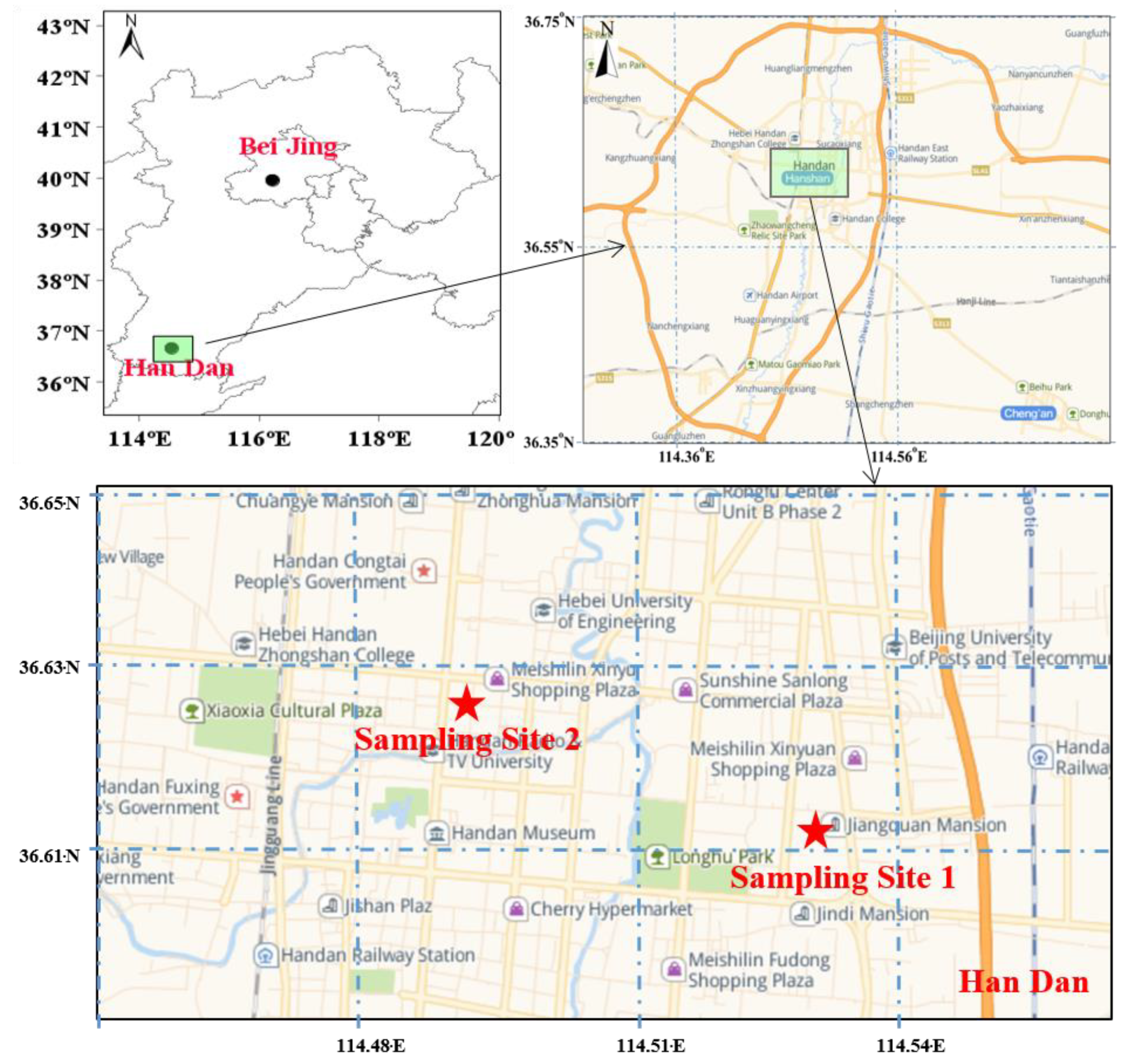
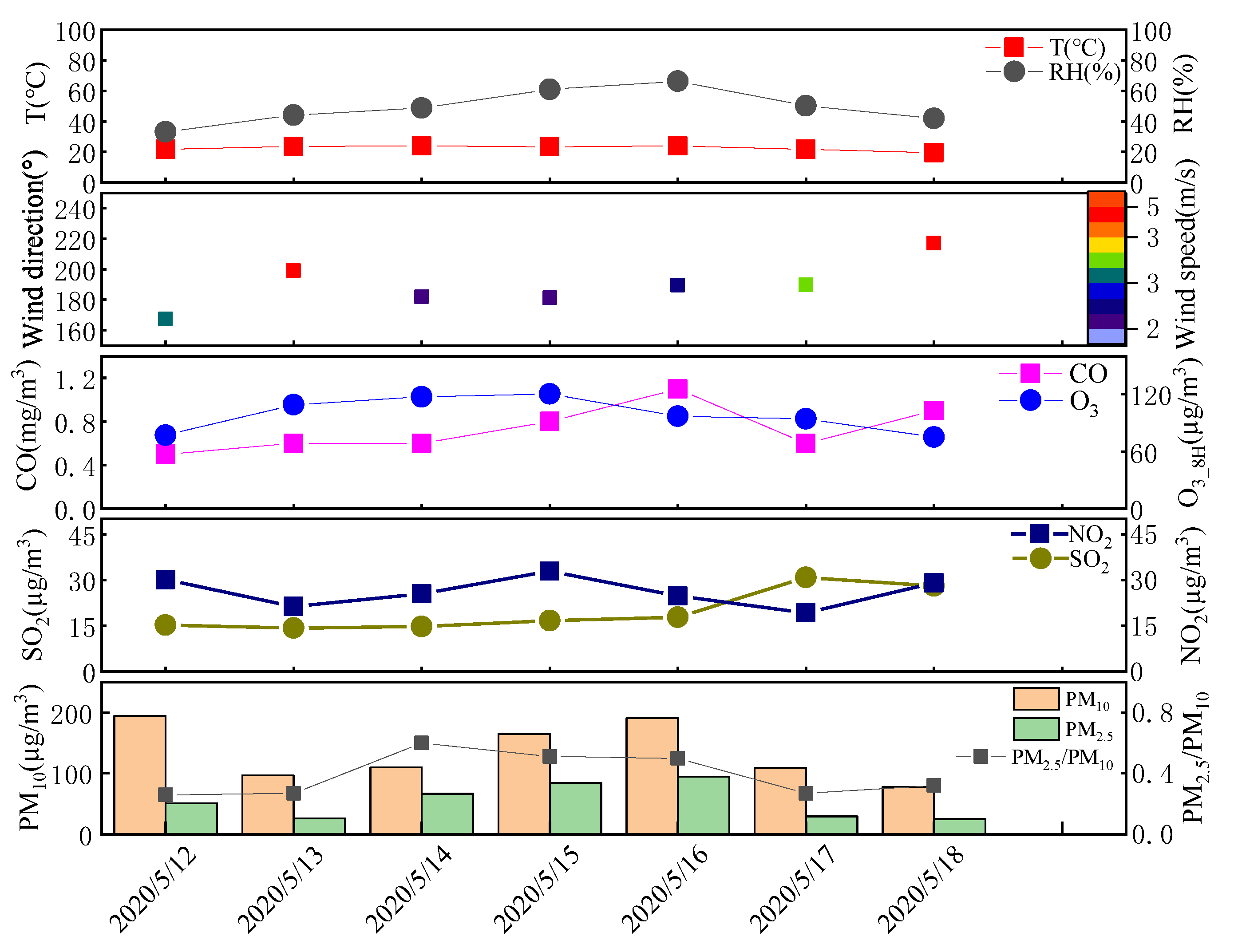
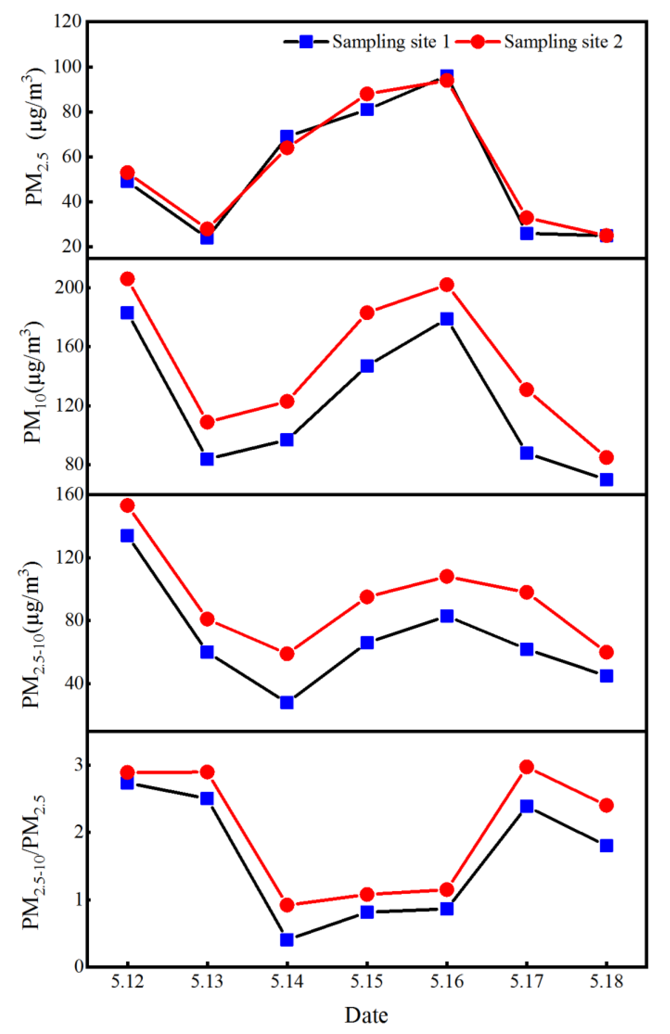
2.1. Sample and Data

Two sampling sites within Handan were selected for the study. Sampling site 1 is located approximately 100 m away from the national control station of the East Wastewater Treatment Plant, with geographic coordinates 36.61° N, 114.53° E. Sampling site 2 is located approximately 1.1 km away from the national control station of Congtai Park in the Hepingli neighborhood, with geographic coordinates 36.62° N, 114.50° E. A schematic diagram of the sampling locations is shown in Figure 1. The Hepingli community is undergoing renovation. The sampling site is 10–20 m from the ground, surrounded by residential areas and parks, and has no tall buildings or industrial sources.

The samples were collected using a Laoying 2034 medium flow sampler adjusted to 100 L/min flow rate, while PM_2.5 and PM₁₀ were collected using quartz filter membranes, which were baked in a muffle furnace at 650 °C for 4 h before use and weighed after constant temperature and humidity treatment. The samples were collected from 12 to 18 May 2020, during the COVID-19 control period. Each sampling period was 23 h long and the membrane diameter was 77 mm. The collected samples were frozen at −20 °C before analysis and 28 effective sampling films were obtained.

2.2. Measures of Variables

The filter membranes were placed in a chamber at constant temperature and humidity for more than 24 h, then weighed after removing static electricity. The membranes were then cut into small pieces of 1.77 cm diameter with a cutting tool, and used for OC/EC, water-soluble ion, and inorganic element analyses. Blank filter membranes were analyzed simultaneously.

2.2.1. OC/EC

The OC/EC content was analyzed with a SUNSET RT-4 carbon analyzer. Briefly, a sample was taken in a quartz tube and the EC/OC content was determined using the protocol NIOSH 5040. The analysis process was as follows: OC (partly carbonized) was detected by continuous volatilization under a He atmosphere. Then, it was detected by the oxidative decomposition of the EC escaping under the He/O₂ environment, and the carbonized OC content was confirmed by the change in laser intensity [67].

2.2.2. Water-Soluble Ion

The contents of eight water-soluble ions (F⁻, Cl⁻, NO₃⁻, SO₄²⁻, NH₄⁺, K⁺, Mg²⁺, and Ca²⁺) were analyzed using a ion chromatograph (DIONEX ICS-1000, Thermo Scientific™, San Diego, CA, USA). Briefly, the sample was placed in a polypropylene vial, soaked in 12 mL ultrapure water for 10 min, and then ultrasonically extracted for 1 h. The sample was filtered through a 0.45 μm filter membrane and then analyzed. The cations and anions were detected on separation columns (IonPac AS23 and IonPac CS12A, Thermo Scientific™, San Diego, CA, USA), respectively.

2.2.3. Elemental

The contents of 19 metals (Ag, Al, Ba, Ca, Cd, Cr, Cu, Fe, K, Mg, Mn, Mo, Ni, Pb, Sr, Ti, V, and Zn) were analyzed by inductively coupled plasma emission spectroscopy (ICPE-9000; Shimadzu, Kyoto, Japan). According to the color depth of the filter membrane, 6–8 pieces were placed in a polytetrafluoroethylene digestion tank. The internal standard (0.010 mL 1000 μg/mL yttrium standard solution) and 5 mL digestion solution (nitric acid:perchloric acid:hydrofluoric acid = 3:1:1) were added and the reflux funnel was covered. The digestion tank was put into the digestion apparatus, and the temperature was raised to 170 °C for 3 h. The reflux funnel was removed and left for 1 h. The tank was then lifted and cooled to room temperature for 30 min. Then, the volume was fixed with 10% nitric acid to 10 mL and analyzed on the machine. This was follows by an analysis of the standard series before the samples were taken, the drawing of standard curves (the correlation coefficient must be more than 0.999), and analysis of the quality control samples (recovery should between 80 and 110%), after which samples could be analyzed. After the testing of 20 samples, a standard solution was analyzed to ensure no major fluctuations from the instrument. A sample blank and laboratory blank were required for every batch.

2.3. Data Analysis Procedure

2.3.1. Enrichment Factor

The enrichment factor (EF) is commonly used to determine whether metal elements in PM are completely derived from crustal elements [68,69], as in Equation (1):

$$EFx=\frac{{\left(C_x/C_{ref}\right)}_{PM}}{{\left(C_x/C_{ref}\right)}_{crust}}$$

(1)

where C_x and C_ref represent the target and reference element concentrations, respectively, and (C_x/C_ref)_PM and (C_x/C_ref)_crust represent the target element to reference element ratio in the PM and the Earth’s crust, respectively, with Ti as the reference element. EF > 1 indicates element enrichment. EF > 5 indicates contributions from anthropogenic sources and EF > 40 indicates extremely high enrichment [70]. The reference values of crustal elements were adopted from a previous study [71].

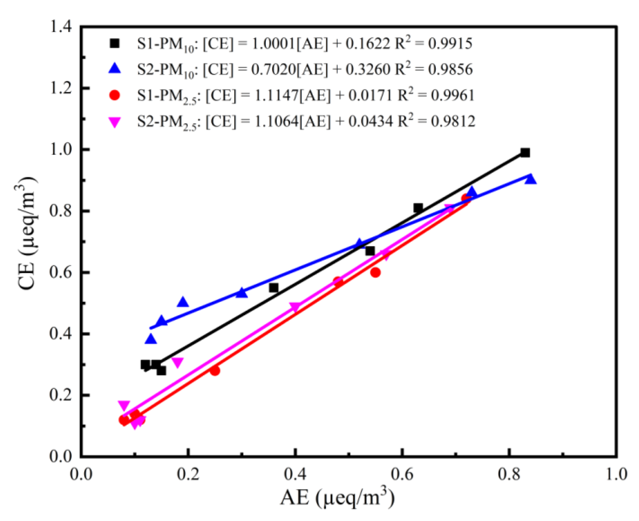
2.3.2. Analysis of Secondary Conversion

The sulfur oxidation rate (SOR) and nitrogen oxidation rate (NOR) can be used to characterize the degree of conversion of SO₂ and NO₂ to SO₄²⁻ and NO₃⁻. Calculations of SOR and NOR were performed according to Equations (2) and (3). When SOR > 0.25 and NOR > 0.10, the greater conversion of SO₂ and NO₂ into SO₄²⁻ and NO₃⁻ occurs in the PM [72]. The SOR and NOR of the PM_2.5 and PM₁₀ at both sampling sites were >0.25, indicating that SO₂ and NO₂ were substantially converted to SO₄²⁻ and NO₃⁻ in the air of Handan City, and controlling the SO₂ and NO₂ emissions could effectively reduce the PM concentration. The formulas are shown in Equations (2) and (3):

$$SOR=\frac{n\left(S{O}_4^{2-}\right)}{n\left(S{O}_4^{2-}\right)+n\left(S{O}_2\right)}$$

(2)

$$NOR=\frac{n\left(N{O}_3^{-}\right)}{n\left(N{O}_3^{-}\right)+n\left(N{O}_2\right)}$$

(3)

2.3.3. PCA-MLR Model

PCA-MLR, with the input of the indicated inorganic and organic source tracers, can quantitatively generate outputs of PM source contributions [73]. Compared with the PMF model, this method requires fewer samples and is more suitable for estimating samples in periods of heavy pollution period [74]. The principle of PCA-MLR analysis is to reduce the dimension, and summarize different components of particulate matter into several specific factors. The calculation process includes the standardization of mass concentration, the calculation of main factors, and the contribution of identified sources; the formulas are shown in Equations (4)–(7):

$$S_{ij}=\left(C_{ij}-C_j\right)/{\sigma }_j$$

(4)

$$F_k={{\displaystyle \sum }}_{j=1}^n{a}_{ij}\times S_{ij}$$

(5)

$$C_{PM}={{\displaystyle \sum }}_{k=1}^m{\beta }_k\times F_k+D$$

(6)

$$\mathsf{ɳ}(\%)=({\beta }_k/{\displaystyle \sum }{\beta }_k)\times 100$$

(7)

In Equation (4), S_ij and C_ij are the standardized value and the mass concentration of the jth composition species in the ith sample, respectively; C_j and σ_j refer to the average mass concentration and the standardized deviation of the jth composition species, respectively. In Equation (5), F_k is the factor score of the kth source; n represents the number of composition species; a_ij and S_ij are the characteristic vector and the standardized value of the jth composition species in the ith sample, respectively. In Equation (6), C_PM is the concentration of PM, m refers to the number of sources, β_k means the regression coefficient of the kth source, and D is the constant value, while $\mathsf{ɳ}$ is the contribution ratio of the factor.

2.3.4. Inhalation Health Risk Assessment

Inhalation health risk assessment is an important tool for assessing the adverse health effects of the exposure of children and adults to air pollutants. Such health risks include carcinogenic risk (CR) resulting from well-defined carcinogenic substances and risk factors (THQ) resulting from non-carcinogenic substances. The carcinogenic risk can be calculated by Equations (8) and (9), as follows:

CR = C × (EF × ED × ET × IUR)/AT

(8)

THQ = Σ(EF × ED × ET × C)/(R_f C × AT × 1000)

(9)

where CR is the carcinogenic risk, C is the components concentration in PM (μg/m³), EF is the exposure frequency (250 day/year), ED is the exposure duration (6 years for children and 24 years for adults), ET is the exposure time (h/day) (8 h/day), AT is the average time of exposure (for non-carcinogens, AT = ED × 365 days × 4 h/day and for carcinogens AT = 70 year × 365 days/year × 24 h), and IUR is inhalation unit risk; the values for carcinogens were taken from USEPA [75].

In general, CR < 1 × 10⁻⁶ indicates that the carcinogenic level caused by the substance poses a negligible risk, and there is no obvious carcinogenic risk. However, when CR > 1 × 10⁻⁴, this indicates that there is an obvious carcinogenic risk, which may lead to health problems. THQ > 1 and THQ < 1 indicate the presence and absence of non-carcinogenic risk, respectively.

2.3.5. Excess Mortality

The Generalized Additive Model (GAM), a traditional mode of time series analysis, was used to estimate the exposure–response relationship between regional air pollutant concentrations and daily mortality. The basic modeling strategy of time series analysis is the same as in the previous study [76]. Based on a zero concentration of air pollutants, an exposure–response model was used to calculate the excess mortality caused by the daily PM₁₀ pollution level during the study period, as shown in Equation (10):

$$E{R}_{kt}=100\times [\left(e^{\beta \times p_{kt}}\right)-1]$$

(10)

where 𝐸𝑅_𝑘𝑡 is excess mortality due to pollutant k on day t, β is the exposure–response relationship coefficient estimated by the regression model, that is, the daily increase in mortality due to each unit increase in the pollutant, and p_kt is the average concentration of the k pollutant on day t.

2.3.6. Potential Source Contribution Function (PSCF)

PSCF analysis identifies the main source areas of atmospheric pollutants based on the analysis of air mass trajectories. We used the meteoinfo software developed by Yaqiang Wang et al. (http://www.meteothink.org/, accessed on 1 December 2022). Meteoinfo can be used to calculate the backward trajectory, determine the spatial distribution of potential pollution sources, and combine this with the concentration of pollutants to calculate the PSCF [77,78]. The PSCF model divides the study area into i × j grids with an accuracy of 0.5° × 0.5° (longitude × latitude), and the PSCF of each grid is calculated as in Equations (11)–(13):

$$PSC{F}_{ij}=\frac{M_{ij}}{N_{ij}}$$

(11)

$$WPSC{F}_{ij}=PSC{F}_{ij}\times W_{ij}$$

(12)

$$W_{ij}=\{\begin{array}{c}1, 80<N_{ij}\\ 0.7, 20<N_{ij}\le 80\\ 0.42, 10<N_{ij}\le 20\\ 0.05, N_{ij}\le 19\end{array}$$

(13)

where Nij is the number of endpoints of trajectory segments on grid ij, and Mij is the number of endpoints of trajectory segments on grid ij with pollutant concentrations higher than the criterion. The threshold value is set to 75 µg/m³, the secondary average daily standard value according to the “China Ambient Air Quality Standard”. To reduce the uncertainty caused by the small Nij in some grids, a weighting factor Wij was introduced as in Equations (12) and (13), and the weighted PSCF value was obtained by multiplying the PSCF value with Wij.

2.3.7. Monitoring Data

Handan’s average daily concentrations of air pollutants such as SO₂, NO₂, O₃ and CO for 2020 were obtained from the China National Environmental Monitoring Station, the East Wastewater Treatment Plant and Congtai Park. Meteorological data were obtained from the China Meteorological Administration, including daily maximum temperature (°C), daily minimum temperature (°C), average temperature (°C), and relative humidity (%). Handan residents’ daily death data in 2020 were obtained from the Chinese Center for Disease Control and Prevention’s cause of death registration and reporting information system, including the sex, age, location and underlying cause of death of the deceased.

3. Results and Discussion

3.1. Characteristics of PM

The time series of PM concentration, gaseous pollutants and meteorological conditions are shown in Figure 2. The average relative humidity is 49%, the average temperature is 22.6 °C, and the prevailing wind direction is southwest wind, with an average wind speed of 3.1 m/s. The average concentration of NO₂ is 26.1 μg/m³, the mean concentration of SO₂ is 19.7 μg/m³, and the average concentration of CO is 0.7 mg/m³, while the mean concentration of O_3-8H is 98.6 μg/m³. All the gaseous pollutants are present at values below the Ambient Air Quality Standard (GB3095-2012). The correlations between pollutants and meteorological favors are shown in Figure S1. The concentration of O_3-8h was significantly correlated with temperature (0.80, p < 0.05), and there is a strong negative correlation between PM_2.5 and wind speed (−0.89, p < 0.01), which means an increase in temperature will lead to much more O_3-8h, and a higher wind speed leads to lower PM concentrations. A lower PM concentration means the virus has no carrier, which will reduce the infection rate of COVID-19 [79].

The concentrations of PM_2.5, PM₁₀, and PM_2.5–10 (aerodynamic diameter between 2.5 and 10 µm, referring to coarse PM) and trends of PM_2.5–10/PM_2.5 at the two sampling sites during the sampling period are shown in Figure 3. The particulate matter increased to the pollution level from a low value at the beginning, and then returned to a low value before the end of sampling, undergoing exactly one pollution process. The PM_2.5, PM₁₀, and PM_2.5–10 concentrations at sampling site 1 were 53 μg/m³ (24–96 μg/m³), 121 μg/m³ (70–183 μg/m³), and 68 μg/m³ (28–134 μg/m³), respectively, with the average PM_2.5–10/PM_2.5 being 1.6 (0.4–2.7). The PM_2.5, PM₁₀, and PM_2.5–10 concentrations at sampling site 2 were 55 μg/m³ (25–95 μg/m³), 148 μg/m³ (85–206 μg/m³), and 93 μg/m³ (59–153 μg/m³), respectively, with the average PM/PM_2.5–10 being 2.0 (0.9–3.0). The PM_2.5–10/PM_2.5 ratio is 1.6 (0.4–2.7) > 0.6 at both sampling sites, which indicates the PM was of the dust type [80]. The PM_2.5 concentration at sampling site 2 was close to that at sampling site 1, but the PM_2.5–10 and PM₁₀ concentrations were significantly higher than those at sampling site 1.

The paired t-test was used to analyze the significant difference in the levels of PM_2.5, PM₁₀ and PM_2.5–10 concentrations between the two sampling sites (Table S1). The PM_2.5 concentrations at the two sampling sites were not significantly different (p = 0.26 > 0.05). However, the PM_2.5–10 and PM₁₀ concentrations at the two sampling sites were significantly different (p = 0.0002 < 0.01 and 0.0001 < 0.01, respectively). This shows that the difference in PM₁₀ concentration between two sampling sites was caused by the PM_2.5–10 concentration. The PM_2.5–10 and PM₁₀ concentrations in sampling site 2 were 25 and 27 μg/m³ higher than those in sampling site 1, respectively, which shows that the PM₁₀ concentration around the old neighborhood increased by 27 μg/m³ due to the renewal of old communities.

Figure S2 shows the results of all measured PM mass concentrations, metal elements, water-soluble ions, and OC/EC concentrations during the sampling period.

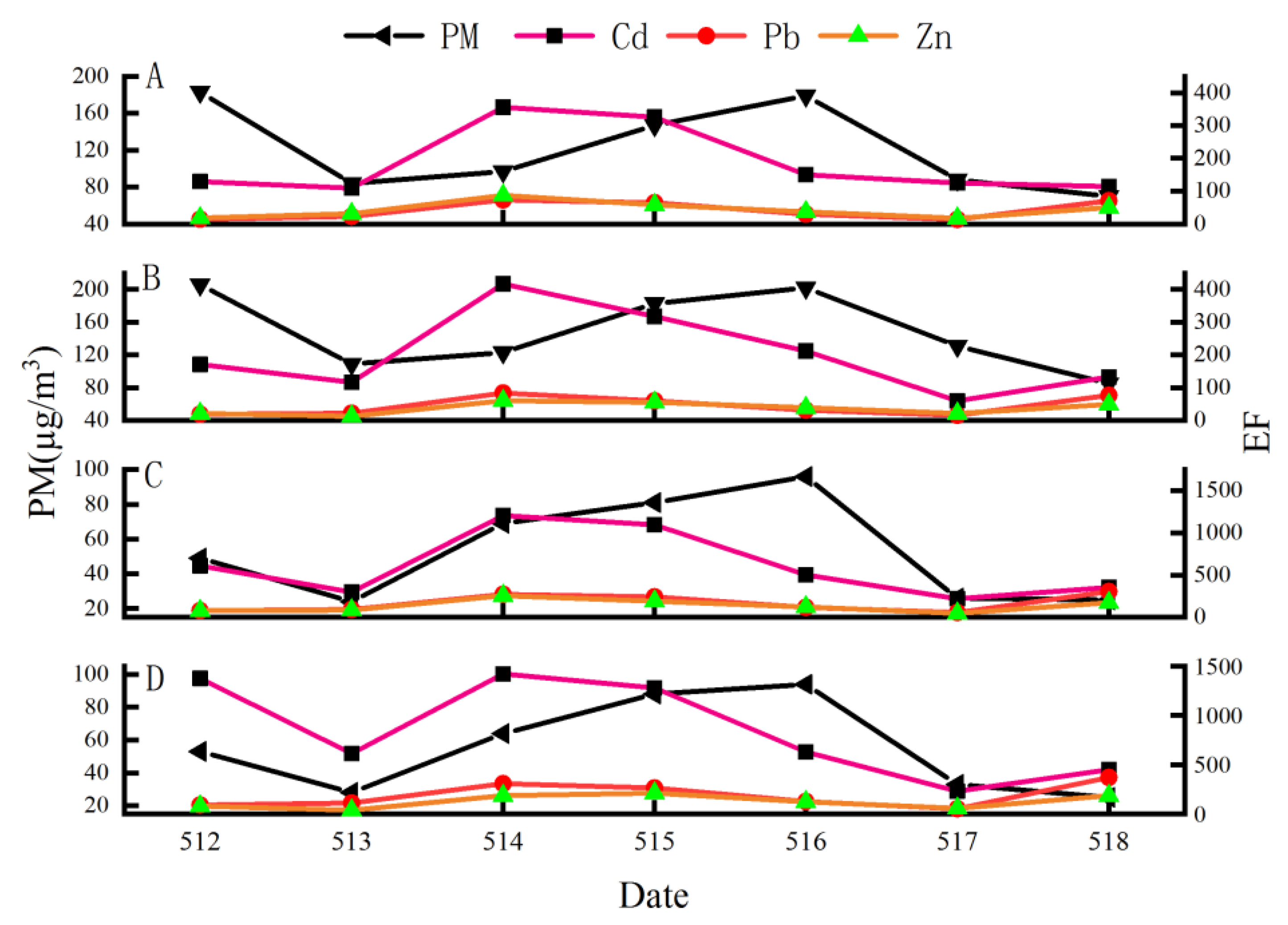
3.1.1. Crustal Elements

The elements in the Earth’s crust mainly include Si, Al, Ca, Fe, Mg, and K. Due to the limitations of the test method, the Si concentration in PM was not tested and was calculated based on the Si/Al ratio in the crust using [Si] = 3.41 [Al] [81]. The concentrations of crustal elements in PM₁₀ at both sampling sites were Si > Ca > Al > Fe > K > Mg > other, and six elements accounted for more than 20% of the PM₁₀ mass concentration, while the other elements accounted for less than 0.5% of PM₁₀ mass concentration. In contrast, the concentrations of crustal elements in PM_2.5 were Si > K > Ca > Al > Fe > Mg > other, with the six elements accounting for about 10% PM_2.5 mass concentration and the contents of the other elements being similar to those in PM₁₀. It can be seen that the crustal elements in PM₁₀ and PM_2.5 had the same sources, except for K, and relatively more K was detected in the fine particles.

The enrichment factors of all determined elements $EFx=\frac{{\left(C_x/C_{ref}\right)}_{PM}}{{\left(C_x/C_{ref}\right)}_{crust}}$ are shown in Table S2. Influenced by the local metallurgical industry, the EF_Cd values in PM₁₀ and PM_2.5 were 212 and 1422, respectively, indicating that the main sources were anthropogenic. In addition, the EF_Pb and EF_Zn were also >40, with a very high enrichment effect, while the enrichment factors of other elements were <5, reflecting no substantial contribution of anthropogenic activities.

The EF_Mn was significantly linearly correlated with EF_Fe (PM₁₀: [EF_Mn] = 1.4646 × [EF_Fe] − 0.3587, R² = 0.8574; PM_2.5: [EF_Mn] = 3.265 × [EF_Fe] − 1.0257, R² = 0.9383), which shows that the Fe and Mn in PM had the same source. However, the slopes of the regression lines in PM₁₀ and PM_2.5 are not consistent, reflecting that the sources in PM_2.5 and PM₁₀ were not consistent. The plot of the trends of enrichment factors and PM concentrations over time (Figure 4) indicates that the enrichment factors peaked two days earlier than the PM concentrations. The crust element is regarded as primary PM; it is assumed that the enrichment of crust element plays an important role in the process of haze formation. Perhaps crust elements can catalyze the generation of secondary PM.

3.1.2. Water-Soluble Ions

Sulfur dioxide (SO₂) and nitrogen oxides (NO_x) produced from fossil fuel combustion are converted to disulfate (SO₄²⁻) and nitrate (NO₃⁻) through heterogeneous reactions under high relative humidity [82], and the presence of ammonia (NH₃) in the air generates secondary ammonium (NH₄⁺) aerosols [83]. SO₄²⁻, NO₃⁻, and NH₄⁺ are collectively referred to as SNA. In addition, the water-soluble ions in PM include inorganic ions such as Ca²⁺, K⁺, Na⁺, Mg²⁺, Cl⁻, and F⁻, and organic ions such as formic acid and oxalate. Water-soluble ions in PM can affect the pH of atmospheric precipitation, reduce atmospheric visibility, and impact human health [84].

The concentrations of common water-soluble ions in PM at the two sampling sites are shown in Table S3. The total water-soluble ion (TWSI) concentrations in PM_2.5 at the two sampling sites were 24.8 and 24.0 µg/m³, respectively, while those in PM₁₀ at the two sampling sites were 32.1 and 34.8 µg/m³, respectively, and the TWSI concentrations as a percentage of the PM_2.5 and PM₁₀ concentrations at sampling sites 1 and 2 were 46.8%, 43.6%, 26.5%, and 23.5%, respectively. These proportions are consistent with those reported previously. The proportion of TWSI in PM_2.5 was substantially higher than that in PM₁₀, indicating a low TWSI concentration in coarse PM. SNA is the main component of TWSI, accounting for more than 90% of the TWSI in PM_2.5, while the SNA proportions in the TWSI in PM₁₀ were 80.1% and 75.9%, which shows that the secondary converted products in SNA were more enriched in fine PM.

The NO₃⁻/SO₄²⁻ in PM is often used to evaluate the contribution of stationary and mobile sources to air quality [85]. NO₃⁻/SO₄²⁻ > 1 indicates that the contribution of mobile sources is higher than that of stationary sources; otherwise, the contribution of stationary sources is greater than that of mobile sources. The NO₃⁻/SO₄²⁻ in the PM_2.5 and PM₁₀ of both sampling sites were >1, indicating that mobile sources contributed more to PM, and controlling mobile sources had a better effect on reducing PM concentrations.

$SOR=\frac{n\left(S{O}_4^{2-}\right)}{n\left(S{O}_4^{2-}\right)+n\left(S{O}_2\right)}NOR=\frac{n\left(N{O}_3^{-}\right)}{n\left(N{O}_3^{-}\right)+n\left(N{O}_2\right)}$. The possible binding forms of SNA in PM are (NH₄)₂SO₄, NH₄HSO₄, NH₄NO₃ or NH₄Cl [86]. To explore the forms present in NH₄⁺ particles, the molar mass relationship between n(NH₄⁺) and n(SO₄²⁻) + n(NO₃⁻) was plotted. n(NH₄⁺) and n(SO₄²⁻) + n(NO₃⁻) were significantly correlated (R > 0.96; p < 0.01 Figure S3). Regardless, SNA is mainly present in the form of (NH₄)₂SO₄ and NH₄NO₃ in both PM₁₀ and PM_2.5. However, the value of n(NH₄⁺) in PM₁₀ is smaller than that of n(SO₄²⁻) + n(NO₃⁻). Ca²⁺ ions in coarse PM compete with NH₄⁺ for SO₄²⁻ to form CaSO₄. As the Ca²⁺ ion concentration in PM₁₀ increases, the CaSO₄ proportion increases, and more NH₄⁺ combines with NO₃⁻ and Cl⁻ to form NH₄NO₃ and NH₄Cl, respectively. However, both NH₄NO₃ and NH₄Cl easily decompose, particularly in summer when the temperature increases; thus, the NH₄⁺ ion concentration in PM₁₀ at the same sampling site was even lower than that in PM_2.5. On the contrary, PM_2.5 was found to be ammonia-rich. In recent years, to reduce NO_x emissions, businesses have been adding urea to the combustion process of diesel engines, increasing NH₃ emissions [87], particularly in non-agricultural cities where the original NH₃ emissions were mainly produced by fossil fuel combustion [88]. As the NH₃ concentration in the air increases, the NH₄⁺ concentration in PM increases, which is more conducive to PM generation, particularly PM₁₀ growth.

The acidity and alkalinity of the PM were calculated according to Equations (14) and (15), and the regression analysis was performed with AE as the abscissa and CE as the ordinate. The correlation coefficients of cations and anions in PM_2.5 at both sampling sites were approximately 1.1 (Figure 5). The amounts of cations were greater than those of anions, causing the solution to be alkaline. The anion and cation concentrations in PM₁₀ at sampling site 1 were the same, thus the slope was 1.0 and the PM was neutral. The anion concentrations were higher than the cation concentrations in PM₁₀ at sampling site 2, thus the PM was acidic. As PM_2.5 grew into PM₁₀, the PM gradually transformed from alkaline to acidic, thus the NH₄⁺ concentration in PM₁₀ was lower than that in PM_2.5.

$$\mathrm{CE} \left(\frac{\mathsf{\mu }\mathrm{eq}}{{\mathrm{m}}^3}\right)=\frac{{\mathrm{Na}}^{+}}{23}+\frac{{\mathrm{NH}}_4^{+}}{18}+\frac{{\mathrm{K}}^{+}}{39}+\frac{{\mathrm{Mg}}^{2+}}{12}+\frac{{\mathrm{Ca}}^{2+}}{20}$$

(14)

$$\mathrm{AE} \left(\frac{\mathsf{\mu }\mathrm{eq}}{{\mathrm{m}}^3}\right)=\frac{{\mathrm{SO}}_4^{2-}}{48}+\frac{{\mathrm{NO}}_3^{-}}{62}+\frac{{\mathrm{Cl}}^{-}}{35.5}+\frac{{\mathrm{F}}^{-}}{19}$$

(15)

3.1.3. Carbon Fractions

The carbonaceous fractions of PM were divided into organic carbon (OC) and elemental carbon (EC), with OC divided into primary organic carbon emitted directly into the atmosphere and secondary organic carbon generated from precursors through photo-oxidation reactions. EC is mainly produced from incomplete fossil fuel or biomass combustion, as well as partially from transportation [89]. The carbonaceous fraction can generally account for 10–50% PM [90], and the OC/EC ratio is often used to indicate the PM source. The OC/EC ratio for biomass combustion is lower than that for fossil fuel combustion products, and the similar OC and EC proportions in TC indicate consistent carbonaceous PM sources [91,92]. An increase in OC concentration in PM implies a decrease in water-soluble ions, and because of the presence of polycyclic aromatic hydrocarbons in OC and the enrichment of elements, the health risk of people exposed to PM will increase [93].

The OC/EC values measured in this study were 1.95–3.23 and 2.58–4.09 for PM₁₀ and PM_2.5, respectively, indicating that the main source of OCEC in PM is coal combustion [94].

3.1.4. PM Reconstruction

By reconstructing the PM mass, the relationship between the chemical component mass concentration and the total PM mass concentration can be understood. The formula for reconstructing the PM mass [95,96,97] has been revised to Equation (16).

RCFM = OM + EC + 1.16 × GM + SNA + Salts + Trace element + others

(16)

where RCFM represents the reconstructed PM mass, OM represents organic matter, EC represents elemental carbon, GM represents mineral content, 1.16 was used to correct for unmeasured compounds, SNA represents secondary inorganic ions, Salts represents sea salt, Trace element represents the trace element, and others represents boundary moisture or loss. In addition to the carbon detected in organic matter, elements such as H, S, O, and N were also present. Therefore, the quantity of OM needs to be multiplied by a factor that varies regionally from 1.4 to 1.8 [98] in terms of organic composition. OM = 1.6 × OC was used in this study. Calculations of GM were performed using Equation (17).

GM = 2.2 × [Al] + 2.49 × [Si] + 1.94 × [Ca] + 1.94 × [Ti] + 2.42 × [Fe] + 2.4 × [K] + 1.66 × [Mg]

(17)

Some studies [99] have used 1.375 [SO₄²⁻] to calculate (NH₄)₂SO₄, and 1.29 [NO₃⁻] to calculate (NH₄)₂SO₄ and NH₄NO₃, instead of NH₄⁺ concentration, provided that both SO₄²⁻ and NO₃⁻ were combined with NH₄⁺ in the PM. The previous analyses show that SO₄²⁻ and NO₃⁻ do not combine completely with NH₄⁺ in the PM, so we added three concentrations for reconstruction. Since Ca is present in mineral dust as CaO and CaCO₃, the coefficient of Ca was calculated using 1.94 [100].

The reconstructed and measured PM values were significantly correlated (R² > 0.96), and the slope was greater than 0.81, except for in the PM₁₀ of sampling site 2 (Figure S4). This indicates that the reconstructed PM accounts for more than 81% of the measured values, and its chemical composition can represent the PM of the measured values. The reconstructed results are consistent with the results reported earlier [101,102]. The reconstructed PM₁₀ of sampling site 2 accounts for 78.2% of the measured values, which shows that under the influence of community renewal, the reconstructed results deviate from the measured values.

3.2. Source Apportionment of PM

To some extent, the correlation between different components in particulate matter can reflect the similarity of their sources [103]. The correlations between the components of PM_2.5 and PM₁₀ are shown in Figure S5. In the figure, red indicates positive correlation, blue indicates negative correlation, larger circles indicate better correlation, and asterisks indicate significant correlation (p < 0.05). The correlations between the components of PM₁₀ in the two sampling sites are better than those of PM_2.5. The correlation between crustal elements such as Al, Fe, K, Mg, Ti, etc., is significant in PM₁₀, but not in PM_2.5. The correlation between secondary pollutants NO₃⁻, SO₄²⁻, NH₄⁺ and OC is good, except for the poor correlation between NH₄⁺ and OC in the PM10 of sampling site 2. A good correlation between Cl⁻ and K indicates that they share common sources.

The results of the PCA of PM show that 85.9% of the total variance can be expressed by three factors.

Table 1. Rotated principal component analysis for components in PM.

Item	F1	F2	F3
OC	0.609	0.663	/
EC	0.839	0.365	0.048
Al	0.976	0.028	0.111
Ca	0.899	0.062	/
Cd	0.29	0.591	0.431
Cr	0.318	/	/
Fe	0.982	0.101	0.055
K	0.93	0.28	0.08
Mg	0.973	0.119	/
Mn	0.976	0.159	0.042
Ni	0.828	0.313	0.246
Pb	0.128	0.791	0.119
Sr	0.984	0.099	/
Ti	0.974	0.065	0.121
V	0.98	0.081	0.053
Zn	0.444	0.834	0.125
Cl−	0.413	/	0.715
NO3−	0.108	0.952	/
SO42−	0.032	0.936	/
Na+	0.636	0.425	/
NH4+	/	0.925	/
Eigenvalue	12.3	4.2	1.6
Variance/%	58.5	19.8	7.6
Cumulative/%	58.5	78.4	85.9

Note: The boldface is the load of the component with larger load in this factor.

shows the load matrix of the PC rotation factor for the components in PM. Al, Ca, Fe, K, Mg, Ti, Fe and V showed higher loads in factor 1 (F1), with the values all higher than 0.82. F1 was considered as a source of dust. The loads of OC, Cd, Pb, Zn, NO₃⁻, SO₄²⁻ and NH₄⁺ were high in factor 2 (F2). F2 was found to mainly contain secondary pollutants, which are oxidized by their precursors of SO₂, NO₂, VOC and NH₃, and Pb is the indicator of motor vehicle source, so F2 was considered as mixed source including secondary transformation, vehicle exhaust and fossil fuels. Factor 3 (F3) contained high levels of Cl⁻, but no K⁺, and this was considered to be a result of COVID-19. The disinfectant used to disinfect COVID-19 is chlorine-rich [104]. We predict that F3 was the source of the high presence of disinfectants, but more research is needed to confirm this.

In order to further quantitatively analyze the main pollution sources and their relative contributions to PM, MLR analysis was performed with the normalized principal factor score as independent variable and PM concentration as the dependent variable, and we derived the regression equation: Z = 0.831F1 + 0.513F2 + 0.031F3. This equation indicates that during the sampling period, the later stage of the COVID-19 epidemic, 60.4% of the PM was contributed by dust, 37.3% by secondary sources, including motor vehicles and industrial coal-fired sources, and the remaining 2.3% was assumed to be derived from disinfectants.

PSCF Analysis

In this study, the 48 h backward trajectory of the air mass from Handan City (36.61° N, 114.19° E, 500 m above ground) from 12 May to 18 May 2020 (during the COVID-19 pandemic) was calculated using meteorological data downloaded from the National Center for Environmental Prediction (NCEP) Global Data Assimilation System (GDAS). The air mass trajectories were clustered into five types using the Euler method (Figure S6). Cluster 1 was short-distance transportation from areas such as Anyang and Kaifeng, contributing 33.93% of the trajectory; cluster 2 was from Inner Mongolia via Shaanxi and southern Henan and Hebei, accounting for 22.2% of the trajectory. Both clusters 1 and 2 reflect the south of Handan City, accounting for 56% of the trajectory; the three trajectories from the northwest of Handan account for 20.8%, 16.7%, and 6.6% of the trajectory, respectively.

The potential source contributions of PM₁₀, PM_2.5, SO₂, and NO₂ in Handan were calculated using PSCF (Figure S6). From Figure S6, it can be seen that the potential PM₁₀ sources were mainly local (WPSCF > 0.7), and the spatial patterns of the potential PM_2.5, SO₂, and NO₂ sources were similar. The main source areas were essentially distributed in southern Hebei, while most of Henan and northern Anhui constituted the potential PM_2.5, SO₂, and NO₂ sources, with relatively high WPSCF. The results of the PSCF calculation are similar to those of previous studies [105,106]; in general, local sources of PM₁₀ in Handan City were significant contributors, while the short-distance transportation of PM_2.5, SO₂, and NO₂ in the southern region was obvious. The results are consistent with the weak southwest wind during the sampling period.

3.3. Health Risk Assessment

Health assessments need to include the concentrations of chromium in trivalent CR (III) and hexavalent CR (VI), whereas the present study measured total concentrations of Cr. We took as reference [107], which assumed a concentration ratio of CR (VI) to CR (III) of 1:6. The carcinogenic and non-carcinogenic risks related to human exposure through inhalation are shown in

Table 2. The carcinogenic risk and non-carcinogenic risks of human exposure to PM.

Risk Source	Children		Adults
	CR	THQ	CR	THQ
PM10 at sampling site 1	5.2 × 10−6	0.56	2.1 × 10−5	0.56
PM10 at sampling site 2	6.9 × 10−6	0.60	2.8 × 10−5	0.60
PM2.5 at sampling site 1	1.0 × 10−6	0.27	1.2 × 10−5	0.27
PM2.5 at sampling site 2	4.4 × 10−6	0.27	5.1 × 10−5	0.27

.

The CR of PM₁₀ in two sampling sites exceeded the acceptable limit of 1 × 10⁻⁶, and the main contributor was CR (VI), as shown in Figure S7. The results are concerning, especially in sampling site 2, where the renewal of old community construction has led to higher values of CR than in sampling site 1. The THQ values of the two sampling sites are both below 1, which implies the absence of non-carcinogenic risk. Hongya Niu’s [108] findings are similar, but Xing Li [109] found that the non-carcinogenic and carcinogenic risks of PM pollution to children exceeded the acceptable limits in almost all cities in Hebei province. The carcinogenic risk of the PAH in particulate matter is generally higher than the acceptable limit in the North China Plain [110]. The health risks associated with PM—especially the carcinogenic risks—are significantly higher than the acceptable limit, and reducing the carcinogens in PM should be the priority when developing control measures.

Excess Mortality

Excess mortality due to PM₁₀ at both sites is shown in Figure 6, which shows that excess mortality was higher at sampling site 2 than at sampling site 1, with an average ΔER 0.11 and a relative increase of 23%. The particulate pollution caused by the renovation of old residential areas not only increases the carcinogenic risk, but also significantly increases the excess mortality.

3.4. Comparison with Other Studies

A comparison of the characteristics, source apportionments and health risk assessments of PM in Handan city in this study with other similar studies is shown in

Table 3. Comparison with other studies on characteristics of PM_2.5.

Item	This Study	Reference [111]	Reference [112]	Reference [62]	Reference [113]
Date	12–18 May 2020	Summer in 2017	23 November–31 December 2020	6–31 December 2015	1–11 July 2016
PM2.5	53 (24–96)	41	124.3	252.4 (58.6–713.1)	77.7
OC/EC	3.2 (2.4–4.1)	-	3.4	3.58 (3.14–4.33)	2.6
ρ (SNA)	22 (5.2–54.0)	50.2 ± 36.1	54.9–60.0	131 (23.4–385.1)	_
ρ (Element)	3.2 (2.3–4.3)	-	_	32.6 (9.3–88.4)	_
ρ (WSI)	24 (6.7–55.4)	53.0 ± 38.1	_	_	_

and

Table 4. Comparison with other studies on source apportionment.

Date	Method	Main Pollution Sources (Proportion)	References
12–18 May 2020	PCA-MLR	Factor 1: dust (60.4 %); Factor 2: mixed source including secondary transformation, vehicle exhaust and fossil fuels (37.3%); Factor 3: assumed to be disinfectants (2.3%)	This study
April–December 2017	PCA	Factor 1: secondary transformation (49.1%); Factor 2: dust (18.5%); Factor 3: coal combustion, biomass burning (13.0%)	[111]
23 November–31 December 2020	PCA	Factor 1: mixed source (37.1%); Factor 2: vehicle exhaust (28.8%)	[112]
6–31 December 2015	PMF	Factor 1: secondary inorganic aerosols (30.3%); Factor 2: coal combustion (26.9%); Factor 3: industrial emissions (15.6%); Factor 4: road dust (10.1%); Factor 5: biomass burning (8.9%); Factor 6: motor vehicles (8.3%)	[62]
5–14 December 2020	PCA	Factor 1: secondary transformation mixed biomass burning (51.2%); Factor 2: dust (26.9%); Factor 3: dust; Factor 4: natural gas combustion source (8.3%)	[113]

.

It can be seen from the comparison that the content of this study is more comprehensive. Studies on PM in Handan generally focus on winter, when air quality is obviously worse than it is in summer. Research on the PM during winter seems to be more valuable. However, during the period of COVID-19, it was found that PM could carry the virus and aggravate its spread, so research on summer PM cannot be neglected.

As regards source apportionment, the main pollution source identified in most of the literature was secondary conversion, or mixed factors such as secondary conversion and motor vehicle and/or coal burning, but dust was the main source in our paper. There are two possible reasons for this: on the one hand, the times of analysis are different—winter is more beneficial to the transformation of secondary pollutants than summer, leading to an increase in the proportional contribution; on the other hand, the contribution of dust to PM may be increased because sampling site 2 in this study is affected by the renewal of old communities. The F3 discovered in this study also differs significantly from other studies.

4. Conclusions

In the latter stage of COVID-19, we chose two sites in Handan to collect PM samples; one of the sites is undergoing community renovation. The characteristics of PM₁₀ and PM_2.5 were to be learned. It was found that the concentration of PM₁₀ increased by 27 μg/m³ during the renovation of the old residential area, which should be of great concern to construction units and the ecological and environmental protection departments. At the same time, the concentration of ammonium in PM₁₀ was lower than that in PM_2.5 at the same sampling site, the mechanism of which requires further study. The source apportionment shows that dust is the most important contributor, accounting for more than 60% of the total, which provides a means of controlling PM. Although the carcinogenic risk caused by PM is no more than 1 × 10⁻⁴, this value is higher than the acceptable limit of 1 × 10⁻⁶, which needs to be taken seriously, because the transformation of old residential areas leads to an increase in PM₁₀ concentration, causing a 23% increase in the excess mortality rate. Meanwhile, PM may be a carrier for viruses; under conditions of low wind speed, the spread of the virus will be accelerated, so it is necessary to take protective measures during periods of pollution.

As sampling took place during the COVID-19 lockdown period, the number of samples is small; more sampling sites and a longer study period are thus needed to improve the accuracy of the results.

References

1. Wu, X.; Xin, J.; Zhang, W.; Gao, W.; Ma, Y.; Ma, Y.; Wen, T.; Liu, Z.; Hu, B.; Wang, Y.; et al. Variation characteristics of air combined pollution in Beijing City. Atmos. Res. 2022, 274, 106197. [Google Scholar] [CrossRef]
2. Fan, F.; Lei, Y.; Li, L. Health damage assessment of PM pollution in Jing-Jin-Ji region of China. Environ. Sci. Pollut. Res. 2019, 26, 7883–7895. [Google Scholar] [CrossRef] [PubMed]
3. Islam, R.; Li, T.; Mahata, K.; Khanal, N.; Werden, B.; Giordano, M.R.; Puppala, S.P.; Dhital, N.B.; Gurung, A.; Saikawa, E.; et al. Wintertime Air Quality across the Kathmandu Valley, Nepal: Concentration, Composition, and Sources of Fine and Coarse Particulate Matter. ACS Earth Space Chem. 2022, 6, 2955–2971. [Google Scholar] [CrossRef] [PubMed]
4. Chowdhury, S.; Pozzer, A.; Haines, A.; Klingmüller, K.; Münzel, T.; Paasonen, P.; Sharma, A.; Venkataraman, C.; Lelieveld, J. Global health burden of ambient PM2.5 and the contribution of anthropogenic black carbon and organic aerosols. Environ. Int. 2022, 159, 107020. [Google Scholar] [CrossRef] [PubMed]
5. Liang, H.; Zhou, X.; Zhu, Y.; Li, D.; Jing, D.; Su, S.; Pan, P.; Liu, H.; Zhang, Y. Association of outdoor air pollution, lifestyle, genetic factors with the risk of lung cancer: A prospective cohort study. Environ. Res. 2023, 218, 114996. [Google Scholar] [CrossRef]
6. VoPham, T.; Jones, R.R. State of the science on outdoor air pollution exposure and liver cancer risk. Environ. Adv. 2023, 11, 100354. [Google Scholar] [CrossRef] [PubMed]
7. Yao, S.; Wang, Q.; Zhang, J.; Zhang, R. Characteristics of Aerosol and Effect of Aerosol-Radiation-Feedback in Handan, an Industrialized and Polluted City in China in Haze Episodes. Atmosphere 2021, 12, 670. [Google Scholar] [CrossRef]
8. Kortoçi, P.; Motlagh, N.H.; Zaidan, M.A.; Fung, P.L.; Varjonen, S.; Rebeiro-Hargrave, A.; Niemi, J.V.; Nurmi, P.; Hussein, T.; Petäjä, T.; et al. Air pollution exposure monitoring using portable low-cost air quality sensors. Smart Health 2022, 23, 100241. [Google Scholar] [CrossRef]
9. Xu, W.; Zhou, W.; Li, Z.; Wang, Q.; Du, A.; You, B.; Qi, L.; Prévôt, A.S.H.; Cao, J.; Wang, Z.; et al. Changes in primary and secondary aerosols during a controlled Chinese New Year. Environ. Pollut. 2022, 315, 120408. [Google Scholar] [CrossRef] [PubMed]
10. Wang, X.; Zhang, Y.; Yang, X. Investigating aerosol chemistry using Real-Time Single Particle Mass Spectrometry: A viewpoint on its recent development. Appl. Geochem. 2023, 149, 105554. [Google Scholar] [CrossRef]
11. Li, H.; Zhang, Q.; Jiang, W.; Collier, S.; Sun, Y.; Zhang, Q.; He, K. Characteristics and sources of water-soluble organic aerosol in a heavily polluted environment in Northern China. Sci. Total Environ. 2021, 758, 143970. [Google Scholar] [CrossRef] [PubMed]
12. Zhang, Q.; Hu, W.; Ren, H.; Yang, J.; Deng, J.; Wang, D.; Sun, Y.; Wang, Z.; Kawamura, K.; Fu, P. Diurnal variations in primary and secondary organic aerosols in an eastern China coastal city: The impact of land-sea breezes. Environ. Pollut. 2023, 319, 121016. [Google Scholar] [CrossRef]
13. Madhavan, S.; Sun, J.; Xiong, X. Sensor calibration impacts on dust detection based on MODIS and VIIRS thermal emissive bands. Adv. Space Res. 2021, 67, 3059–3071. [Google Scholar] [CrossRef]
14. Wang, H.; Chai, S.; Tang, X.; Zhou, B.; Bian, J.; Vömel, H.; Yu, K.; Wang, W. Verification of satellite ozone/temperature profile products and ozone effective height/temperature over Kunming, China. Sci. Total Environ. 2019, 661, 35–47. [Google Scholar] [CrossRef] [PubMed]
15. Baruah, U.D.; Robeson, S.M.; Saikia, A.; Mili, N.; Sung, K.; Chand, P. Spatio-temporal characterization of tropospheric ozone and its precursor pollutants NO2 and HCHO over South Asia. Sci. Total Environ. 2022, 809, 151135. [Google Scholar] [CrossRef] [PubMed]
16. Xiong, X.; Liu, X.; Wu, W.; Knowland, K.E.; Yang, Q.; Welsh, J.; Zhou, D.K. Satellite observation of stratospheric intrusions and ozone transport using CrIS on SNPP. Atmos. Environ. 2022, 273, 118956. [Google Scholar] [CrossRef]
17. Semlali, B.-E.B.; El Amrani, C.; Ortiz, G.; Boubeta-Puig, J.; Garcia-De-Prado, A. SAT-CEP-monitor: An air quality monitoring software architecture combining complex event processing with satellite remote sensing. Comput. Electr. Eng. 2021, 93, 107257. [Google Scholar] [CrossRef]
18. Wang, Y.; Yin, Z.; Zheng, Z.; Li, J.; Li, Q.; Meng, C.; Li, W. Spatial-temporal Distribution and Evolution Characteristics of Air Pollution in Beijing-Tianjin-Hebei Region Based on Long-term “Ground-Satellite” Data. Environ. Sci. 2022, 43, 3508–3522. [Google Scholar]
19. Sarwar, G.; Hogrefe, C.; Henderson, B.-H.; Foley, K.; Mathur, R.; Murphy, B.; Ahmed, S. Characterizing variations in ambient PM2.5 concentrations at the U.S. Embassy in Dhaka, Bangladesh using observations and the CMAQ modeling system. Atmos. Environ. 2023, 296, 119587. [Google Scholar] [CrossRef]
20. Cholakian, A.; Bessagnet, B.; Menut, L.; Pennel, R.; Mailler, S. Anthropogenic Emission Scenarios over Europe with the WRF-CHIMEREv2020 Models: Impact of Duration and Intensity of Reductions on Surface Concentrations during the Winter of 2015. Atmosphere 2023, 14, 224. [Google Scholar] [CrossRef]
21. Salva, J.; Vanek, M.; Schwarz, M.; Gajtanska, M.; Tonhauzer, P.; Duricová, A. An Assessment of the On-Road Mobile Sources Contribution to Particulate Matter Air Pollution by AERMOD Dispersion Model. Sustainability 2021, 13, 12748. [Google Scholar] [CrossRef]
22. Zhang, K.; Leeuw, G.-d.; Yang, Z.; Chen, X.; Su, X.; Jiao, J. Estimating Spatio-Temporal Variations of PM2.5 Concentrations Using VIIRS-Derived AOD in the Guanzhong Basin, China. Remote Sens. 2019, 11, 2679. [Google Scholar] [CrossRef] [Green Version]
23. Chen, C.-C.; Wang, Y.-R.; Yeh, H.-Y.; Lin, T.-H.; Huang, C.-S.; Wu, C.-F. Estimating monthly PM2.5 concentrations from satellite remote sensing data, meteorological variables, and land use data using ensemble statistical modeling and a random forest approach. Environ. Pollut. 2021, 291, 118159. [Google Scholar] [CrossRef] [PubMed]
24. Zhou, W.; Wu, X.; Ding, S.; Ji, X.; Pan, W. Predictions and mitigation strategies of PM2.5 concentration in the Yangtze River Delta of China based on a novel nonlinear seasonal grey model. Environ. Pollut. 2021, 276, 116614. [Google Scholar] [CrossRef] [PubMed]
25. Lv, L.; Wei, P.; Li, J.; Hu, J. Application of machine learning algorithms to improve numerical simulation prediction of PM2.5 and chemical components. Atmos. Pollut. Res. 2021, 12, 101211. [Google Scholar] [CrossRef]
26. Dai, H.; Huang, G.; Zeng, H.; Yang, F. PM2.5 Concentration Prediction Based on Spatiotemporal Feature Selection Using XGBoost-MSCNN-GA-LSTM. Sustainability 2021, 13, 12071. [Google Scholar] [CrossRef]
27. Bera, B.; Bhattacharjee, S.; Sengupta, N.; Saha, S. PM2.5 concentration prediction during COVID-19 lockdown over Kolkata metropolitan city, India using MLR and ANN models. Environ. Chall. 2021, 4, 100155. [Google Scholar] [CrossRef]
28. Dai, H.; Huang, G.; Zeng, H.; Zhou, F. PM2.5 volatility prediction by XGBoost-MLP based on GARCH models. J. Clean. Prod. 2022, 356, 131898. [Google Scholar] [CrossRef]
29. Dai, H.; Huang, G.; Zeng, H.; Yu, R. Haze Risk Assessment Based on Improved PCA-MEE and ISPO-LightGBM Model. Systems 2022, 10, 263. [Google Scholar] [CrossRef]
30. Fadel, M.; Ledoux, F.; Afif, C.; Courcot, D. Human health risk assessment for PAHs, phthalates, elements, PCDD/Fs, and DL-PCBs in PM2.5 and for NMVOCs in two East-Mediterranean urban sites under industrial influence. Atmos. Pollut. Res. 2022, 1, 101261. [Google Scholar] [CrossRef]
31. Diffenbaugh, N.S.; Field, C.B.; Appel, E.A.; Azevedo, I.L.; Baldocchi, D.D.; Burke, M.; Burney, J.A.; Ciais, P.; Davis, S.J.; Fiore, A.M.; et al. The COVID-19 lockdowns: A window into the Earth System. Nat. Rev. Earth Environ. 2020, 1, 470–481. [Google Scholar] [CrossRef]
32. Niu, H.; Shi, L.; Ren, X.; Jin, N.; Wang, S.; Li, S.; Hu, S.; Wu, C.; Lu, Y.; Fan, J.; et al. Chemical characteristics of particulate matter in the atmospheric environment after “coal substitution” policy in coal combustion cities and their surrounding areas. J. China Coal Soc. 2022, 47, 4362–4374. [Google Scholar]
33. Suman, R.; Javaid, M.; Choudhary, S.K.; Haleem, A.; Singh, R.P.; Nandan, D.; Ali, S.; Rab, S. Impact of COVID-19 Pandemic on Particulate Matter (PM) concentration and harmful gaseous components on Indian metros. Sustain. Oper. Comput. 2021, 2, 1–11. [Google Scholar] [CrossRef]
34. Donzelli, G.; Cioni, L.; Cancellieri, M.; Morales, A.L.; Suárez-Varela, M.M.M. The Effect of the COVID-19 Lockdown on Air Qualityin Three Italian Medium-Sized Cities. Atmosphere 2020, 11, 1118. [Google Scholar] [CrossRef]
35. Seo, J.H.; Jeon, H.W.; Sung, U.J.; Sohn, J.-R. Impact of the COVID-19 Outbreak on Air Quality in Korea. Atmosphere 2020, 11, 1137. [Google Scholar] [CrossRef]
36. Sulaymon, I.D.; Zhang, Y.; Hopke, P.K.; Hu, J.; Zhang, Y.; Li, L.; Mei, X.; Gong, K.; Shi, Z.; Zhao, B.; et al. Persistent high PM2.5 pollution driven by unfavorable meteorological conditions during the COVID-19 lockdown period in the Beijing-Tianjin-Hebei region, China. Environ. Res. 2021, 198, 111186. [Google Scholar] [CrossRef] [PubMed]
37. Ou, S.; Wei, W.; Cheng, S.; Cai, B. Exploring drivers of the aggravated surface O3 over North China Plain in summer of 2015–2019: Aerosols, precursors, and meteorology. J. Environ. Sci. 2023, 127, 453–464. [Google Scholar] [CrossRef]
38. Pozzer, A.; Dominici, F.; Haines, A.; Witt, C.; Münzel, T.; Lelieveld, J. Regional and global contributions of air pollution to risk of death from COVID-19. Cardiovasc. Res. 2020, 116, 2247–2253. [Google Scholar] [CrossRef] [PubMed]
39. Carballo, I.H.; Bakola, M.; Stuckler, D. The impact of air pollution on COVID-19 incidence, severity, and mortality: A systematic review of studies in Europe and North America. Environ. Res. 2022, 215, 114155. [Google Scholar] [CrossRef]
40. Coccia, M. Factors determining the diffusion of COVID-19 and suggested strategy to prevent future accelerated viral infectivity similar to COVID. Sci. Total Environ. 2020, 729, 138474. [Google Scholar] [CrossRef]
41. Coccia, M. How do low wind speeds and high levels of air pollution support the spread of COVID-19? Atmos. Pollut. Res. 2021, 12, 437–445. [Google Scholar] [CrossRef]
42. Tian, Y.; Wang, X.; Zhao, P.; Shi, Z.; Harrison, R.M. PM2.5 Source Apportionment using Organic Marker-based CMB Modeling: Influence of Inorganic Markers and Sensitivity to Source Profiles. Atmos. Environ. 2023, 294, 119477. [Google Scholar] [CrossRef]
43. Huang, R.; Li, Z.; Ivey, C.E.; Zhai, X.; Shi, G.; Mulholland, J.A.; Devlin, R.; Russell, A.G. Application of an improved gas-constrained source apportionment method using data fused fields: A case study in North Carolina, USA. Atmos. Environ. 2022, 276, 119031. [Google Scholar] [CrossRef]
44. Liu, Y.; Yang, Z.; Liu, Q.; Qi, X.; Qu, J.; Zhang, S.; Wang, X.; Jia, K.; Zhu, M. Study on chemical components and sources of PM2.5 during heavy air pollution periods at a suburban site in Beijing of China. Atmos. Pollut. Res. 2021, 12, 188–199. [Google Scholar] [CrossRef]
45. Yuan, C.-S.; Wong, K.-W.; Tseng, Y.-L.; Ceng, J.-H.; Lee, C.-E.; Lin, C. Chemical significance and source apportionment of fine particles (PM2.5) in an industrial port area in East Asia. Atmos. Pollut. Res. 2022, 13, 101349. [Google Scholar] [CrossRef]
46. Zhang, Z.; Xu, B.; Xu, W.; Wang, F.; Gao, J.; Li, Y.; Li, M.; Feng, Y.; Shi, G. Machine learning combined with the PMF model reveal the synergistic effects of sources and meteorological factors on PM2.5 pollution. Environ. Res. 2022, 212, 113322. [Google Scholar] [CrossRef] [PubMed]
47. Dai, Q.; Ding, J.; Song, C.; Liu, B.; Bi, X.; Wu, J.; Zhang, Y.; Feng, Y.; Hopke, P.H. Changes in source contributions to particle number concentrations after the COVID-19 outbreak: Insights from a dispersion normalized PMF. Sci. Total Environ. 2021, 759, 143548. [Google Scholar] [CrossRef]
48. Xu, H.; Xiao, Z.; Chen, K.; Tang, M.; Zheng, N.; Li, P.; Yang, N.; Yang, W.; Deng, X. Spatial and temporal distribution, chemical characteristics, and sources of ambient PM in the Beijing-Tianjin-Hebei region. Sci. Total Environ. 2019, 658, 280–293. [Google Scholar] [CrossRef] [PubMed]
49. Huang, X.; Liu, Z.; Liu, J.; Hu, B.; Wen, T.; Tang, G.; Zhang, J.; Wu, F.; Ji, D.; Wang, L.; et al. Chemical characterization and source identification of PM2.5 at multiple sites in the Beijing–Tianjin–Hebei region, China. Atmos. Chem. Phys. 2017, 17, 12941–12962. [Google Scholar] [CrossRef]
50. Ma, J.; Shen, J.; Wang, P.; Zhu, S.; Wang, Y.; Wang, P.; Wang, G.; Chen, J.; Zhang, H. Modeled changes in source contributions of particulate matter during the COVID-19 pandemic in the Yangtze River Delta, China. Atmos. Chem. Phys. 2021, 21, 7343–7355. [Google Scholar] [CrossRef]
51. Li, J.; Xie, X.; Li, L.; Wang, X.; Wang, H.; Jing, S.; Ying, Q.; Qin, M.; Hu, J. Fate of Oxygenated Volatile Organic Compounds in the Yangtze River Delta Region: Source Contributions and Impacts on the Atmospheric Oxidation Capacity. Environ. Sci. Technol. 2022, 56, 11212–11224. [Google Scholar] [CrossRef]
52. Yang, S.; Ma, Y.; Duan, F.; He, K.; Wang, L.; Wei, Z.; Zhu, L.; Ma, T.; Li, H.; Ye, S. Characteristics and formation of typical winter haze in Handan, one of the most polluted cities in China. Sci. Total Environ. 2018, 613–614, 1367–1375. [Google Scholar] [CrossRef]
53. The Ministry of Ecology and Environment Reported the National Surface Water and Ambient Air Quality in December and January–December 2021, 2022. Available online: https://www.mee.gov.cn/ywdt/xwfb/202201/t20220131_968703.shtml (accessed on 20 October 2022).
54. Wang, Q.; Hou, Z.; Li, L.; Guo, S.; Liang, H.; Li, M.; Luo, H.; Wang, L.; Luo, Y.; Ren, H. Seasonal disparities and source tracking of airborne antibiotic resistance genes in Handan, China. J. Hazard. Mater. 2022, 422, 126844. [Google Scholar] [CrossRef] [PubMed]
55. Cai, A.; Zhang, H.; Wang, L.; Wang, Q.; Wu, X. Source apportionment and health risk assessment of heavy metals in PM2.5 in Handan: A typical heavily polluted city in North China. Atmosphere 2021, 12, 1232. [Google Scholar] [CrossRef]
56. Cheng, M.; Zhang, H.; Wan, L. Spatial and temporal disribution characterustics of PM2.5 and variation factors of the AQI in the Beijing-Tianjin-Hebei region from 2015 to 2018. Appl. Ecol. Environ. Res. 2020, 5, 4441–4458. [Google Scholar] [CrossRef]
57. Liu, Y.; Zhang, Y.; Zhang, Y.; Liang, Y.; Zhu, X.; Lan, J.; Niu, H.; Fan, J. Comparison of air quality index (AQI) before and after COVID-19 in Handan City and analysis of air pollution characteristics during COVID-19 prevention and control. Environ. Chem. 2021, 40, 3743–3754. [Google Scholar]
58. Yang, H.; Tao, W.; Liu, Y.; Qiu, M.; Liu, J.; Jiang, K.; Yi, K.; Xiao, Y.; Tao, S. The contribution of the Beijing, Tianjin and Hebei region’s iron and steel industry to local air pollution in winter. Environ. Pollut. 2019, 245, 1095–1106. [Google Scholar] [CrossRef] [PubMed]
59. Zhao, Z.; Qi, Y.; Han, R.; Xiao, N.; Li, J. Changes in the emission of dust particles from soil in the Beijing-Tianjin-Hebei region in the past 20 years. Acta Ecol. Sin. 2022, 42, 7910–7920. [Google Scholar]
60. Li, M.; Yu, S.; Chen, X.; Li, Z.; Zhang, Y.; Song, Z.; Liu, W.; Li, P.; Zhang, X.; Zhang, M.; et al. Impacts of condensable PM on atmospheric organic aerosols and fine PM (PM2.5) in China. Atmos. Chem. Phys. 2022, 22, 11845–11866. [Google Scholar] [CrossRef]
61. Meng, C.; Wang, L.; Zhang, F.; Wei, Z.; Ma, S.; Ma, X.; Yang, J. Characteristics of concentrations and water-soluble inorganic ions in PM2.5 in Handan City, Hebei province, China. Atmos. Res. 2016, 171, 133–146. [Google Scholar] [CrossRef]
62. Chen, C.; Zhang, H.; Li, H.; Wu, N.; Zhang, Q. Chemical characteristics and source apportionment of ambient PM1.0 and PM2.5 in a polluted city in North China plain. Atmos. Environ. 2020, 242, 117867. [Google Scholar] [CrossRef]
63. Yan, H.; Ding, G.; Feng, K.; Zhang, L.; Li, H.; Wang, Y.; Wu, T. Systematic evaluation framework and empirical study of the impacts of building construction dust on the surrounding environment. J. Clean. Prod. 2020, 275, 122767. [Google Scholar] [CrossRef]
64. Shi, J.; Zhang, W.; Guo, S.; An, H. Numerical Modelling of Blasting Dust Concentration and Particle Size Distribution during Tunnel Construction by Drilling and Blasting. Metals 2022, 12, 547. [Google Scholar] [CrossRef]
65. Zhang, Y.; Tang, W.; Li, H.; Guo, J.; Wu, J.; Guo, Y. The Evaluation of Construction Dust Diffusion and Sedimentation Using Wind Tunnel Experiment. Toxics 2022, 10, 412. [Google Scholar] [CrossRef] [PubMed]
66. Yan, H.; Ding, G.; Li, H.; Wang, Y.; Zhang, L.; Shen, Q.; Feng, K. Field Evaluation of the Dust Impacts from Construction Sites on Surrounding Areas: A City Case Study in China. Sustainability 2019, 11, 1906. [Google Scholar] [CrossRef] [Green Version]
67. Karanasiou, A.; Panteliadis, P.; Perez, N.; Minguillón, M.; Pandolfi, M.; Titos, G.; Viana, M.; Moreno, T.; Querol, X.; Alastuey, A. Evaluation of the Semi-Continuous OCEC analyzer performance with the EUSAAR2 protocol. Sci. Total Environ. 2020, 747, 141266. [Google Scholar] [CrossRef] [PubMed]
68. Thiombane, M.; Di Bonito, M.; Albanese, S.; Zuzolo, D.; Lima, A.; de Vivo, B. Geogenic versus anthropogenic behaviour and geochemical footprint of Al, Na, K and P in the Campania region (Southern Italy) soils through compositional data analysis and EF. Geoderma 2019, 335, 12–26. [Google Scholar] [CrossRef] [Green Version]
69. Lin, Y.-C.; Li, Y.-C.; Amesho, K.T.; Shangdiar, S.; Chou, F.-C.; Cheng, P.-C. Chemical characterization of PM2.5 emissions and atmospheric metallic element concentrations in PM2.5 emitted from mobile source gasoline-fueled vehicles. Sci. Total Environ. 2020, 15, 139942. [Google Scholar] [CrossRef] [PubMed]
70. Mancilla, Y.; Paniagua, H.I.Y.; Mendoza, A. Spatial differences in ambient coarse and fine particles in the Monterreymetropolitan area, Mexico: Implications for source contribution. J. Air Waste Manag. Assoc. 2019, 69, 548–564. [Google Scholar] [CrossRef] [Green Version]
71. Wedepohl, K.H. The composition of the continental crust. Geochim. Cosmochim. Acta 1995, 59, 1217–1232. [Google Scholar] [CrossRef]
72. Wang, S.; Yin, S.; Zhang, R.; Yang, L.; Zhao, Q.; Zhang, L.; Yan, Q.; Jiang, N.; Tang, X. Insight into the formation of secondary inorganic aerosol based on high-time-resolution data during haze episodes and snowfall periods in Zhengzhou, China. Sci. Total Environ. 2019, 660, 47–56. [Google Scholar] [CrossRef]
73. Zhou, H.; Lü, C.; He, J.; Gao, M.; Zhao, B.; Ren, L.; Zhang, L.; Fan, Q.; Liu, T.; He, Z.; et al. Stoichiometry of water-soluble ions in PM2.5: Application in source apportionment for a typical industrial city in semi-arid region, Northwest China. Atmos. Res. 2018, 204, 149–160. [Google Scholar] [CrossRef]
74. Zhao, B.; Xu, J.; Zhang, G.; Lu, S.; Liu, X.; Li, L.; Li, M. Occurrence of antibiotics and antibiotic resistance genes in the Fuxian Lake and antibiotic source analysis based on principal component analysis-multiple linear regression model. Chemosphere 2021, 262, 127741. [Google Scholar] [CrossRef]
75. Risk Assessment Guidance for Superfund (RAGS): Part F. Available online: https://www.epa.gov/risk/risk-assessment-guidance-superfund-rags-part-f (accessed on 1 February 2023).
76. Wang, Y.; Ding, D.; Ji, X.; Zhang, X.; Zhou, P.; Dou, Y.; Dan, M.; Shu, M. Construction of Multipollutant Air Quality Health Index and Susceptibility Analysis Based on Mortality Risk in Beijing, China. Atmosphere 2022, 13, 1370. [Google Scholar] [CrossRef]
77. Wang, Y.Q. An Open Source Software Suite for Multi-Dimensional Meteorological Data Computation and Visualisation. J. Open Res. Softw. 2019, 7, 21. [Google Scholar] [CrossRef] [Green Version]
78. Wang, Y.Q. MeteoInfo: GIS software for meteorological data visualization and analysis. Meteorol. Appl. 2014, 21, 360–368. [Google Scholar] [CrossRef]
79. Coccia, M. The effects of atmospheric stability with low wind speed and of air pollution on the accelerated transmission dynamics of COVID-19. Int. J. Environ. Stud. 2021, 78, 1. [Google Scholar] [CrossRef]
80. Fan, H.; Zhao, C.; Yang, Y.; Yang, X. Spatio-Temporal Variations of the PM2.5/PM10 Ratios and Its Application to Air Pollution Type Classification in China. Front. Environ. Sci. 2021, 9, 692440. [Google Scholar] [CrossRef]
81. Mason, B. Principles of Geochemistry, 3rd ed.; John Wiley & Sons, Inc.: New York, NY, USA, 1966. [Google Scholar]
82. Huang, X.; Liu, Z.; Zhang, J.; Wen, T.; Ji, D.; Wang, Y. Seasonal variation and secondary formation of size-segregated aerosol water-soluble inorganic ions during pollution episodes in Beijing. Atmos. Res. 2016, 168, 70–79. [Google Scholar] [CrossRef]
83. Hannun, R.M.; Razzaq, A.H.A. Air Pollution Resulted from Coal, Oil and Gas Firing in Thermal Power Plants and Treatment: A Review. IOP Conf. Ser. Earth Environ. Sci. 2022, 1002, 012008. [Google Scholar] [CrossRef]
84. Zhang, Y.-X.; Cao, F.; Zheng, H.; Zhang, D.-D.; Zhai, X.-Y.; Fan, M.-Y.; Zhang, Y.-L. Pollution source and health risk assessment of polycyclic aromatic hydrocarbons in PM2.5 in Changchun City in autumn of 2017. Huan Jing Ke Xue 2020, 41, 564–573. (In Chinese) [Google Scholar]
85. Chen, Y.; Wang, Y.; Nenes, A.; Wild, O.; Song, S.; Hu, D.; Liu, D.; He, J.; Ruiz, L.H.; Apte, J.S.; et al. Ammonium Chloride Associated Aerosol Liquid Water Enhances Haze in Delhi, India. Environ. Sci. Technol. 2022, 56, 7163–7173. [Google Scholar] [CrossRef]
86. Mehregan, M.; Moghiman, M. Experimental investigation of the distinct effects of nanoparticles addition and urea-SCR after-treatment system on NOx emissions in a blended-biodiesel fueled internal combustion engine. Fuel 2020, 262, 116609. [Google Scholar] [CrossRef]
87. Viatte, C.; Petit, J.-E.; Yamanouchi, S.; Van Damme, M.; Doucerain, C.; Germain-Piaulenne, E.; Gros, V.; Favez, O.; Clarisse, L.; Coheur, P.-F.; et al. Ammonia and PM2.5 Air Pollution in Paris during the 2020 COVID Lockdown. Atmosphere 2021, 12, 160. [Google Scholar] [CrossRef]
88. Pan, Y.; Tian, S.; Liu, D.; Fang, Y.; Zhu, X.; Gao, M.; Gao, J.; Michalski, G.; Wang, Y. Isotopic evidence for enhanced fossil fuel sources of aerosol ammonium in the urban atmosphere. Environ. Pollut. 2018, 238, 942–947. [Google Scholar] [CrossRef]
89. Li, M.; Bao, F.; Zhang, Y.; Song, W.; Chen, C.; Zhao, J. Role of elemental carbon in the photochemical aging of soot. Proc. Natl. Acad. Sci. USA 2018, 115, 7717–7722. [Google Scholar] [CrossRef] [Green Version]
90. Duarte, R.M.; Mieiro, C.L.; Penetra, A.; Pio, C.A.; Duarte, A.C. Carbonaceous materials in size-segregated atmospheric aerosols from urban and coastal-rural areas at the Western European Coast. Atmos. Res. 2008, 90, 253–263. [Google Scholar] [CrossRef]
91. Tian, J.; Ni, H.; Cao, J.; Han, Y.; Wang, Q.; Wang, X.; Chen, L.-W.; Chow, J.C.; Watson, J.G.; Wei, C.; et al. Characteristics of carbonaceous particles from residential coal combustion and agricultural biomass burning in China. Atmos. Pollut. Res. 2017, 17, 521–527. [Google Scholar] [CrossRef]
92. Wu, C.; Yu, J.Z. Determination of primary combustion source organic carbon-to-elemental carbon (OC/EC) ratio using ambient OC and EC measurements: Secondary OC-EC correlation minimization method. Atmos. Chem. Phys. 2016, 16, 5453–5465. [Google Scholar] [CrossRef] [Green Version]
93. Zhang, M.; Li, Z.; Xu, M.; Yue, J.; Cai, Z.; Yung, K.K.L.; Li, R. Pollution characteristics, source apportionment and health risks assessment of fine PM during a typical winter and summer time period in urban Taiyuan, China. Hum. Ecol. Risk Assess. 2019, 10, 2737–2750. [Google Scholar]
94. Chen, Y.; Zhi, G.; Feng, Y.; Fu, J.; Feng, J.; Sheng, G.; Simoneit, B.R.T. Measurements of emission factors for primary carbonaceous particles from residential raw-coal combustion in China. Geophys. Res. Lett. 2006, 33, L20815. [Google Scholar] [CrossRef]
95. Malm, W.C.; Sisler, J.F.; Huffman, D.; Eldred, R.A.; Cahill, T. Spatial and seasonal trends in particle concentration and optical extinction in the United States. J. Geophys. Res. Atmos. 1994, 99, 1347–1370. [Google Scholar] [CrossRef]
96. Agarwal, A.; Satsangi, A.; Lakhani, A.; Kumari, K.M. Seasonal and spatial variability of secondary inorganic aerosols in PM2.5 at Agra: Source apportionment through receptor models. Chemosphere 2020, 242, 125132. [Google Scholar] [CrossRef] [PubMed]
97. Zhang, Y.; Sartelet, K.; Zhu, S.; Wang, W.; Wu, S.-Y.; Zhang, X.; Wang, K.; Tran, P.; Seigneur, C.; Wang, Z.-F. Application of WRF/Chem-MADRID and WRF/Polyphemus in Europe—Part 2: Evaluation of chemical concentrations and sensitivity simulations. Atmos. Chem. Phys. 2013, 13, 6845–6875. [Google Scholar] [CrossRef] [Green Version]
98. Chow, J.C.; Lowenthal, D.H.; Chen, L.-W.A.; Wang, X.; Watson, J.G. Mass reconstruction methods for PM2.5: A review. Air Qual. Atmos. Health 2015, 8, 243–263. [Google Scholar] [CrossRef] [Green Version]
99. Liao, W.; Zhou, J.; Zhu, S.; Xiao, A.; Li, K.; Schauer, J.J. Characterization of aerosol chemical composition and the reconstruction of light extinction coefficients during winter in Wuhan, China. Chemosphere 2020, 241, 125033. [Google Scholar] [CrossRef]
100. Remoundaki, E.; Kassomenos, P.; Mantas, E.; Mihalopoulos, N.; Tsezos, M. Composition and Mass Closure of PM2.5 in Urban Environment (Athens, Greece). Aerosol Air Qual. Res. 2013, 13, 72–82. [Google Scholar] [CrossRef] [Green Version]
101. Zou, J.; Liu, Z.; Hu, B.; Huang, X.; Wen, T.; Ji, D.; Liu, J.; Yang, Y.; Yao, Q.; Wang, Y. Aerosol chemical compositions in the North China Plain and the impact on the visibility in Beijing and Tianjin. Atmos. Res. 2018, 201, 235–246. [Google Scholar] [CrossRef]
102. Wang, Y.-S.; Chang, L.-C.; Chang, F.-J. Explore Regional PM2.5 Features and Compositions Causing Health Effects in Taiwan. Environ. Manag. 2021, 67, 176–191. [Google Scholar] [CrossRef]
103. Qiao, B.; Chen, Y.; Tian, M.; Wang, H.; Yang, F.; Shi, G.; Zhang, L.; Peng, C.; Luo, Q.; Ding, S. Characterization of water soluble inorganic ions and their evolution processes during PM2.5 pollution episodes in a small city in southwest China. Sci. Total Environ. 2019, 650, 2605–2613. [Google Scholar] [CrossRef] [PubMed]
104. United States Environmental Protection Agency. List N: Products with Emerging Viral Pathogens AND Human Coronavirus Claims for Use against SARS-CoV-2. Available online: https://www.epa.gov/sites/default/files/2020-06/documents/sars-cov2_listn_06122020.pdf (accessed on 6 December 2020).
105. Li, H.; Zhang, Q.; Zhang, Q.; Chen, C.; Wang, L.; Wei, Z.; Zhou, S.; Parworth, C.; Zheng, B.; Canonaco, F.; et al. Wintertime aerosol chemistry and haze evolution in an extremely polluted city of the North China Plain: Significant contribution from coal and biomass combustion. Atmos. Chem. Phys. 2017, 17, 4751–4768. [Google Scholar] [CrossRef] [Green Version]
106. Zhang, C.; Wang, L.L.; Qi, M.; Ma, X.; Zhao, L.; Ji, S.; Wang, Y.; Lu, X.; Wang, Q.; Xu, R.; et al. Evolution of Key Chemical Components in PM2.5 and Potential Formation Mechanisms of Serious Haze Events in Handan, China. Aerosol Air Qual. Res. 2018, 18, 1545–1557. [Google Scholar] [CrossRef] [Green Version]
107. Li, H.; Wang, J.; Wang, Q.; Qian, X.; Qian, Y.; Yang, M.; Li, F.; Lu, H.; Wang, C. Chemical fractionation of arsenic and heavy metals in fine particle matter and its implications for risk assessment: A case study in Nanjing, China. Atmos. Environ. 2015, 103, 339–346. [Google Scholar] [CrossRef]
108. Niu, H.; Wu, Z.; Xue, F.; Liu, A.; Hu, W.; Wang, J.; Fan, J.; Lu, Y. Seasonal variations and risk assessment of heavy metals in PM2.5 from Handan, China. World J. Eng. 2021, 18, 886–897. [Google Scholar] [CrossRef]
109. Li, X.; Yan, C.; Wang, C.; Ma, J.; Li, W.; Liu, J.; Liu, Y. PM2.5-bound elements in Hebei Province, China: Pollution levels, source apportionment and health risks. Sci. Total Environ. 2022, 806, 150440. [Google Scholar] [CrossRef]
110. Gong, X.; Shen, Z.; Zhang, Q.; Zeng, Y.; Sun, J.; Ho, S.S.H.; Lei, Y.; Xu, H.; Cui, S.; Huang, Y.; et al. Characterization of polycyclic aromatic hydrocarbon (PAHs) source profiles in urban PM2.5 fugitive dust: A large-scale study for 20 Chinese cites. Sci. Total Environ. 2019, 687, 188–197. [Google Scholar] [CrossRef]
111. Ren, X.; Niu, H.; Li, S.; Xue, F.; Wu, Z.; Fan, J. Pollution characteristics and source of water-soluble ions in atmospheric fine particles in Handan City. Environ. Chem. 2021, 40, 3510–3519. [Google Scholar]
112. Ren, X.L.; Hu, W.; Wu, C.M.; Hu, S.H.; Gao, N.N.; Zhang, C.C.; Yue, L.; Wang, J.X.; Fan, J.S.; Niu, H.Y. Chemical Characteristics and Sources of Atmospheric Aerosols in the Surrounding District of a Heavily Polluted City in the Southern Part of North China. Environ. Sci. 2022, 43, 1159–1169. [Google Scholar]
113. Xue, F.; Niu, H.; Wu, Z.; Ren, X.; Li, S.; Wang, J.; Yue, L.; Fan, J. Pollution characteristics of organic carbon and elemental carbon in PM2.5 and PM10 of Handan City. Environ. Chem. 2021, 40, 3246–3257. [Google Scholar]
Figure 1. Schematic diagram of sampling locations.
Atmosphere 14 00680 g001
Figure 2. Time series of PM concentration, gaseous pollutants and meteorological conditions.
Atmosphere 14 00680 g002
Figure 3. PM2.5, PM10, and PM2.5–10 concentrations and changes in PM2.5–10/PM2.5 at both sampling sites.
Atmosphere 14 00680 g003
Figure 4. Relationship between Cd, Pb and Zn enrichment factors and particle concentration over time (A: the PM10 of sample site 1; B: the PM10 of sample site 2; C: the PM2.5 of sample site 1; D: the PM2.5 of sample site 2).
Atmosphere 14 00680 g004
Figure 5. Relationship between AE and CE in PM.
Atmosphere 14 00680 g005
Figure 6. The excess mortality caused by PM10 between the two sampling sites.
Atmosphere 14 00680 g006