
Examining the Impact of Dimethyl Sulfide Emissions on Atmospheric Sulfate over the Continental U.S.
by
 , ,
, ,
Golam Sarwar
1,*, 
Daiwen Kang
1,
Barron H. Henderson
2,
Christian Hogrefe
1,
Wyat Appel
1 and
Rohit Mathur
1 1
Center for Environmental Measurement and Modeling, Office of Research and Development, U.S. Environmental Protection Agency, Durham, NC 27711, USA
2
Office of Air Quality Planning and Standards, U.S. Environmental Protection Agency, Durham, NC 27711, USA
*
Author to whom correspondence should be addressed.
Atmosphere 2023, 14(4), 660; https://doi.org/10.3390/atmos14040660
Submission received: 20 January 2023
/
Revised: 26 March 2023
/
Accepted: 29 March 2023
/
Published: 31 March 2023
(This article belongs to the Section Air Quality)
Abstract
:We examined the impact of dimethylsulfide (DMS) emissions on sulfate concentrations over the continental U.S. by using the Community Multiscale Air Quality (CMAQ) model version 5.4 and performing annual simulations without and with DMS emissions for 2018. DMS emissions enhance sulfate not only over seawater but also over land, although to a lesser extent. On an annual basis, the inclusion of DMS emissions increase sulfate concentrations by 36% over seawater and 9% over land. The largest impacts over land occur in California, Oregon, Washington, and Florida, where the annual mean sulfate concentrations increase by ~25%. The increase in sulfate causes a decrease in nitrate concentration due to limited ammonia concentration, especially over seawater, and an increase in ammonium concentration with a net effect of increased inorganic particles. The largest sulfate enhancement occurs near the surface (over seawater), and the enhancement decreases with altitude, diminishing to 10–20% at an altitude of ~5 km. Seasonally, the largest enhancement in sulfate over seawater occurs in summer, and the lowest in winter. In contrast, the largest enhancements over land occur in spring and fall due to higher wind speeds that can transport more sulfate from seawater into land.
1. Introduction
Sulfate is an important component of atmospheric fine particles and can also affect the cloud condensation nuclei and the aerosol radiative forcing [1,2,3,4]. Sulfate is formed in the atmosphere mainly from the oxidation of sulfur dioxide (SO2) via gas- and aqueous-phase chemistry. Sulfur can be emitted from natural as well as anthropogenic sources. Significant reductions in anthropogenic SO2 emissions from fossil fuel combustion have occurred in the U.S. during the past decades due to stringent control measures in response to tightened air quality standards. For example, the U.S. Environmental Protection Agency (EPA) reported a 93% reduction in anthropogenic SO2 emissions during 1980–2021 despite a 187% increase in gross domestic product, 111% increase in vehicle miles travelled, and 25% increase in energy consumption during the same period (https://www.epa.gov/air-trends/air-quality-national-summary#air-quality-trends (accessed on 24 August 2022)). Similar changes have occurred in many other parts of the world [5]. The contribution of sulfate to fine particles varies with time and location. Tanner et al. [6] analyzed trends in annual pollutant concentrations in eastern Tennessee and reported that ammonium sulfate contributed 48% in 1999 and 41% in 2013 to fine particle mass concentrations in Look Rock, Tennessee. Malm et al. [7] performed an analysis of measured sulfate concentrations at the IMPROVE (Interagency Monitoring of Protected Visual Environments) sites for 2001–2015 and reported that, on average, ammonium sulfate contributed 30% to the summertime reconstructed fine particle mass. There are some specific regions in the U.S. where other species contribute a substantial fraction to fine particle mass. For example, aerosol nitrate and organic aerosol contribute ~85% of wintertime fine particle mass in San Joaquin Valley in California [8]. Atmospheric sulfate concentrations in the U.S. have decreased over the years; however, they are still an important constituent of fine particles.
Dimethyl sulfide (DMS; CH3SCH3) can be emitted from natural as well as anthropogenic sources. Natural sources of DMS include emissions from the ocean, wetlands, and plants and soil, with the ocean being the largest source [9]. Phytoplankton in seawater [9] contain dimethylsulfoniopropionate (DMSP), which produces DMS upon breakdown. DMS emissions can also be emitted from anthropogenic sources. For example, paper and pulp industries and rayon/cellulosics manufacturing facilities can emit DMS; however, their emissions are an order of magnitude lower than natural emissions [10]. Estimates of oceanic DMS emissions range between 17.6 and 34.4 Tg S yr−1 [3] and are ~10 times larger than the anthropogenic DMS emission estimates of 2.20 Tg S yr−1 [10]. Once emitted into the atmosphere, the oxidation of DMS forms sulfur-containing products such as SO2 and sulfuric acid [11,12]. These products then lead to the formation of sulfate aerosols. While the anthropogenic sulfur emissions are decreasing, natural sulfur emissions remain mostly unchanged. Thus, natural oceanic DMS emissions play an increasingly important role in the atmosphere, and their impact on sulfate needs a careful examination. Several previous studies have been conducted to examine the impact of natural sulfur emissions on sulfate [3,13,14,15,16,17,18,19,20]. However, most of these studies employed global or hemispheric models and were conducted with older modeling systems for historic conditions which did not reflect recent decreases in anthropogenic sulfur emissions and/or covered only limited areas over the U.S. For example, Park and coworkers [13] used the GEOS-Chem version 5.03 model (geos-chem.seas.harvard.edu) with a horizontal resolution of 2° × 2.5° and conducted simulations for 2001. They included natural sulfur emissions from oceans, volcanoes, and biomass burning sources and reported that these emissions can enhance ammonium sulfate concentrations in the U.S. Zhao et al. [20] implemented oceanic DMS emissions in the CMAQv5.3 modeling system [21]. Using the hemispheric Community Multiscale Air Quality (CMAQ) model (www.epa.gov/cmaq, accessed on 15 December 2022) version 5.3 with 108 km horizontal grids, they reported that DMS emissions can enhance surface sulfate concentration over many areas of the northern hemisphere, including the U.S., but they did not conduct any regional-scale CMAQ simulations. In one of the two previous regional-scale modeling studies we are aware of, Mueller et al. [18] applied CMAQv4.6 with a horizontal resolution of 36 × 36 km for 2002 atmospheric conditions to examine the impact of natural emissions on sulfate. They included natural sulfur emissions from the ocean, coastal wetlands, freshwater lakes, the Great Salt Lake, soil, and geothermal sources; performed simulations over the continental U.S., Canada, Mexico, and surrounding oceanic areas; and reported that these emissions can enhance ammonium sulfate over the U.S. Perraud et al. [19] examined the impacts of a hypothetical scenario with zero anthropogenic SO2 emissions in a large coastal urban area in California. They applied a three-dimensional air quality model (The University of California, Irvine—California Institute of Technology regional airshed model) with 5 km horizontal grids over California and reported that particle formation would be reduced by two orders of magnitude in the case of zero anthropogenic SO2 emissions; however, particles would continue to form from natural and anthropogenic sources of organosulfur compounds. In this study, we add to this body of knowledge generated in earlier studies by examining the impact of oceanic DMS emissions on sulfate over the continental U.S. for recent atmospheric conditions using the latest version of CMAQ (version 5.4) with horizontal grid spacings of 12 km and constrained by lateral boundary conditions from corresponding large-scale CMAQv5.4 simulations performed over the northern hemisphere.
2. Materials and Methods
To quantify the impact of oceanic DMS, we used a simulation without DMS emissions (NODMS) and a simulation with DMS emission (WDMS). They both shared the base model configuration and emissions (except DMS). The WDMS simulation used the on-line implementation of DMS emissions, while the NODMS simulation did not use the on-line DMS emissions. Both simulations included additional chemistry implemented for DMS. The base model configuration, the additional chemistry, and DMS emissions implementations are described below.
2.1. Base Model Configuration
CMAQ is a state-of-the-science three-dimensional chemical transport model containing detailed treatments of important atmospheric processes. It has been widely used in the U.S. and many other countries for air quality simulations involving research as well as regulatory activities [21,22,23,24,25]. Here, we used the recently released CMAQv5.4 [26] for simulating air quality for the entire year of 2018. The modeling domain covered the entire continental U.S., parts of Canada and Mexico, and surrounding oceanic areas with 12 km horizontal grid spacings and 35 vertical layers of varying thickness with a surface layer height of 20 m. The modeling domain contained a total of 459 × 299 × 35 (4,803,435) grid cells. Meteorological fields were generated using the Weather Research and Forecasting (WRFv4.3.3, [27]) model with the RRTMG (Rapid Radiative Transfer Model for GCMs) for long- and short-wave radiation [28], Kain–Fritsch scheme [29] with lightning assimilation [30,31] for convective parameterization, Morrison microphysics scheme [32], Pleim–Xiu land surface model [33,34], and the Asymmetric Convective Model version 2 (ACM2; [35,36]) for the planetary boundary layer (PBL) scheme. Four-dimensional data assimilation (FDDA) using “analysis nudging” was applied to continuously nudge the wind, temperature, and water vapor mixing ratio above the PBL [37] toward the NAM 12 km analysis every three hours. The Meteorology Chemistry Interface Processor (MCIPv5.3.3) [38] was used to process the WRF results into CMAQ-ready input files. Torres-Vazquez et al. [39] compared WRFv4.1.1 predictions with observed data over the U.S. (same modeling domain used in this study) and reported model performance for wind speed, wind direction, temperature, and mixing ratios. The model configuration between the two studies is same, except that we used WRFv4.3.3 and they used WRFv4.1.1. The WRF model performance in this study is similar to that reported by Torres-Vazquez et al. [39]. We employed the standard cloud and aero7 modules, and the Carbon Bond chemical mechanism (version 6, release 5 (CB6r5)) [40] with chlorine chemistry [41].
The model included emissions from various natural and anthropogenic sources. Anthropogenic source emissions include contributions from mobile, point, and non-point sources and were obtained from the 2017 National Emissions Inventory and projected for 2018. Additional information on different types of emissions can be found in EPA [42]. Mobile source emissions include contributions from on- and off-road vehicles, commercial marine vessels, and railroads. Point source emissions include contributions from electric generating units, oil and gas facilities, industrial sources not included in electric generating units and oil/gas facilities, agricultural field burning activities, wild/prescribed burning activities, and airports. Non-point source emissions include contributions from agriculture, area fugitive dust, oil and gas facilities, residential wood combustion, and others. In addition, emissions from Mexico and Canada were also included. The details of these emissions can be found at the EPA website (www.epa.gov/cmaq/equates#emissions_modeling, accessed on 10 December 2022). Biogenic emissions were calculated using the in-line Biogenic Emission Inventory System (BEIS4). In-line sea-salt spray emissions were calculated following Gantt et al. [43], while in-line lightning emissions were calculated following Kang et al. [44]. The simulation in this study did not include any wind-blown dust emissions.
2.2. DMS Emission Implementation
In addition, we included DMS flux (F) from the ocean, estimated using the total gas transfer velocity () and the DMS concentration in seawater () (F) as follows [3]:
DMS concentrations in seawater can be obtained from several databases [3,45,46]. Here, we used the monthly climatological seawater concentration from the Surface Ocean and Lower Atmosphere project (www.bodc.ac.uk/solas_integration/implementation_products/group1/dms, accessed on 26 April 2022) [3] for calculating the DMS flux. The in Equation (1) is calculated using the water side gas transfer velocity () and the atmospheric gradient fraction () as follows:
can be estimated using several parameterizations [47,48,49]. Lana et al. [3] estimated global DMS emissions using these parameterizations and reported that the Wanninkhof [49] parameterization produces the highest estimates, and the Liss and Merlivat [47] parameterization produces the minimum estimates. Consistent with the study of Zhao et al. [20], for the northern hemisphere, we also used the Liss and Merlivat [47] parameterization (Equation (3)) to calculate DMS flux.
The Schmidt number () describes the diffusion of DMS in seawater and is calculated using sea surface temperature (,)
[50]:
The atmospheric gradient fraction, , can be calculated using Equation (5):
H is dimensionless Henry’s Law Coefficient (liquid/gas) and can be calculated as follows:
where is the universal gas constant (0.08205746 atm L/K mol), is the sea surface temperature, and is the solubility of DMS:
The wind-speed-dependent airside transfer coefficient, is defined by
where is the molecular weight of DMS and is the molecular weight of water [51].
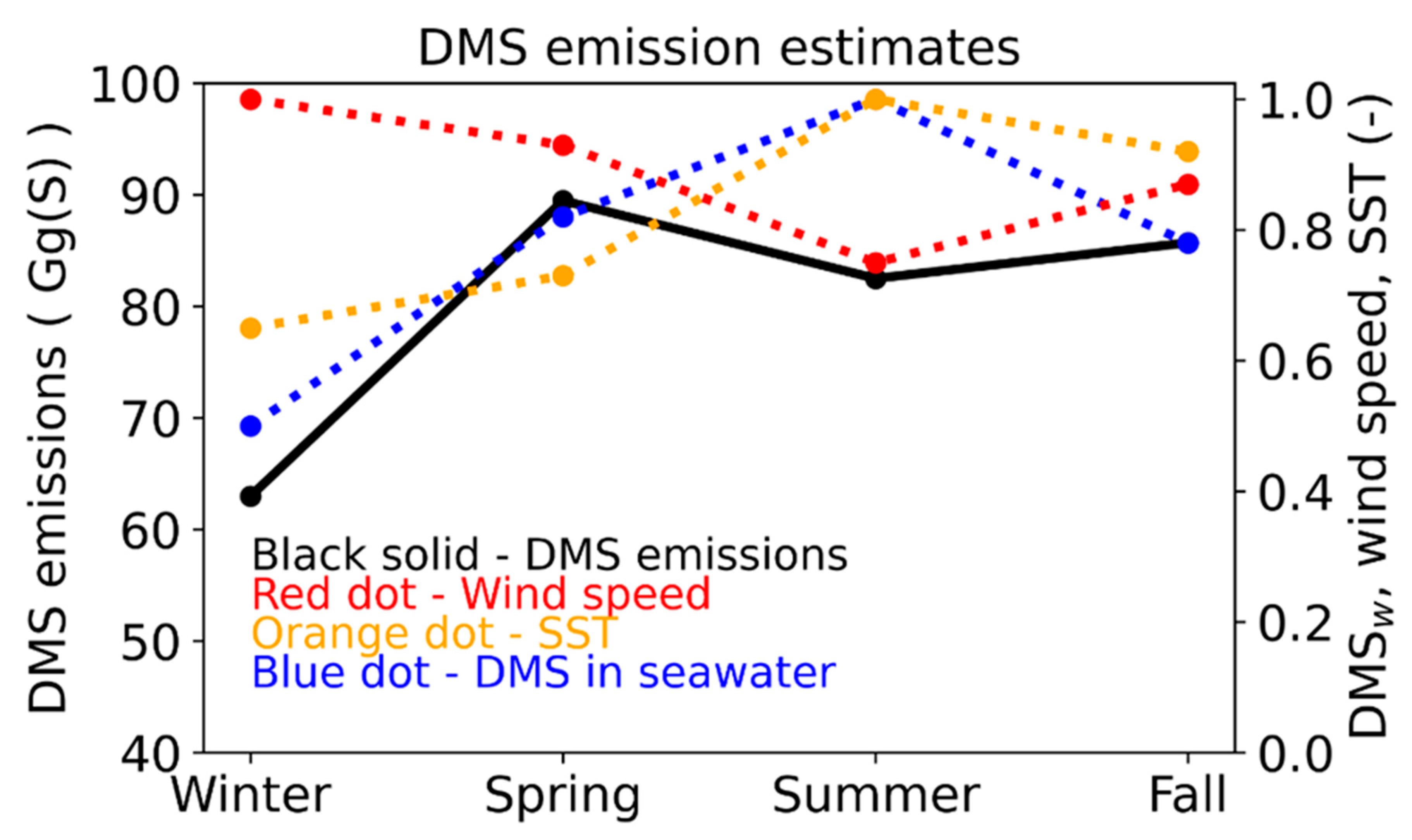
Seasonal DMS emissions (estimated using the scheme described above) over the modeling domain (only grid cells emitting DMS emissions are used for the calculation) are shown in Figure 1. The highest estimate (89.5 Gg(S)—gigagram of sulfur) occurred in spring (March–May) and the lowest (62.9 Gg(S)) in winter. DMS emissions estimates in summer (June–August) and fall (September–November) were lower than those in spring, but higher than those in winter (December–February). Mean DMS concentration in seawater, wind speed, and sea surface temperature (SST) are also shown in Figure 1. DMS emissions increased with higher DMS concentrations in seawater, higher wind speed, and higher SST. Both the DMS concentration in seawater and SST were the highest in summer and the lowest in winter. However, wind speed was the highest in winter and the lowest in summer. Summertime DMS emissions were lower than those in spring due to lower wind speed. The lowest DMS emissions in winter were driven by the lowest DMS concentration in seawater and SST. The annual DMS emissions were 320 Gg(S) with ~21 Gg(S) in January and ~29 Gg(S) in July. Smith and Mueller [52] used a similar domain extent and reported 18 Gg(S) in January and 45 Gg(S) in July. January emissions estimates between the two studies vary by <20%, while July emissions estimates vary by ~50%, likely due to the differences in the temporal allocation of annual emissions between the two studies.
2.3. DMS Chemistry Implementation
DMS chemistry was previously implemented in the hemispheric CMAQ model [20]. Seven chemical reactions involving the oxidation of DMS by hydroxyl radical (OH), nitrate radical (NO3), chlorine radical (Cl), chlorine oxide (ClO), bromine oxide (BrO), and iodine oxide (IO) were used in the hemispheric CMAQ model. The CB6r5 chemical mechanism does not include any bromine or iodine chemistry; thus, the reactions of DMS with BrO and IO were not included in this study. In addition, since the reaction of ClO only contributes ~0.1% of the total DMS oxidation [20], it was also excluded in this study. As shown in Table 1, four chemical reactions for DMS oxidation were included. DMS chemistry produces SO2, which is then further oxidized by gas-phase reaction with OH to produce sulfate aerosol. The in-cloud oxidation of SO2 by hydrogen peroxide (H2O2), ozone (O3), methyl hydroperoxide (MEPX), peroxyacetic acid (PACD), and oxygen catalyzed by iron (Fe[III]) and manganese (Mn[II]) further produces aerosol sulfate.
2.4. Boundary Conditions
Boundary conditions were generated from the hemispheric CMAQ model [56] simulations using CMAQv5.4. Two different model simulations were performed using the hemispheric CMAQv5.4: one simulation without DMS emissions and the other with DMS emissions. Results obtained with these hemispheric simulations were used to prepare two different sets of boundary conditions for the 12 km modeling domain for this study. The first 12 km simulation contained no DMS emissions and used the hourly boundary condition derived from the hemispheric model without DMS emissions (NODMS); the second 12 km simulation contained DMS emissions and used the hourly boundary condition derived from the hemispheric model with DMS emissions (WDMS). The differences in the model results are thus solely attributable to the DMS emissions that occur in both the 12 km and hemispheric domain. Initial conditions for the model were prepared using results from a previously generated model simulation for the EPA’s Air Quality Time Series (EQUATES) (www.epa.gov/cmaq/equates, accessed on 12 October 2022). The simulation was started on 22 December 2017 and continued until 31 December 2018. The simulations for the first 10 days were used for the spin-up purpose. The analyses of the model results were performed for the entire year of 2018.
3. Results and Discussion
3.1. Annual Impact of DMS Emissions on Surface Inorganic Particles
Predicted annual mean changes (WDMS—NODMS) in surface sulfate, nitrate, ammonium, and total inorganic (sulfate + nitrate + ammonium) particle concentrations due to DMS emissions are shown in Figure 2. DMS emissions enhance sulfate concentrations not only over seawater but also over land area. The largest enhancements occur over seawater and then gradually decrease over the interior portion of the modeling domain. DMS is emitted from the ocean and has a relatively short lifetime (~0.5 day; [57]); thus, the highest enhancements occur over seawater. The impact is particularly high over the Pacific Ocean due in part to the prevailing wind direction carrying the impact of western boundary conditions into the modeling domain. DMS emissions enhance sulfate concentrations by 0.10–0.50 μg/m3 (12–67%) over a large portion of seawater, with a mean over-ocean enhancement of 0.24 µg/m3 (36%). DMS emissions also enhance sulfate concentrations by 0.05–0.25 μg/m3 over a large area of land, with a mean enhancement of 0.055 µg/m3 (9%). The impacts near coastal areas are greater than those over the interior portion of land. The largest impacts over land occur in coastal areas of Washington, Oregon, California, southern Texas, and Florida, in which they generally increase sulfate in some areas by more than 30–40%. They also increase sulfate by up to ~50% in some grid cells along the coastal areas. Considering the entire state, DMS emissions increase annual mean sulfate by 0.15 µg/m3 (23%) over Florida, 0.11 µg/m3 (24%) over California, 0.09 µg/m3 (25%) over Oregon, 0.09 µg/m3 (25%) over Washington, and 0.09 µg/m3 (9%) over Texas. While the impacts over some coastal states are relatively large, the impacts over many interior states covering large areas of the modeling domain are relatively small (<0.05 μg/m3; ~4–6%).
DMS emissions decrease nitrate concentrations by 0.04–0.28 μg/m3 (6–67%) over seawater and 0–0.28 μg/m3 (0–69%) over coastal areas and increase ammonium concentrations by up to 0.04 μg/m3 (~14% at the location of the maximum increase). Overall, they decrease mean nitrate by 0.13 µg/m3 (39%) over the entire seawater and 0.016 µg/m3 (5%) over the entire land area and increase annual mean ammonium by 0.013 µg/m3 (35%) over the entire seawater and 0.012 µg/m3 (7%) over the entire land area. Ammonia preferentially reacts with sulfuric acid, forming ammonium sulfate or bisulfate [9]. Any remaining ammonia then reacts with nitric acid, forming ammonium nitrate. Ammonia concentrations, especially over seawater, tend to be limited and are consumed by the additional sulfuric acid produced by DMS emissions, increasing both the ammonium and sulfate concentrations and decreasing nitrate concentrations. Ammonium nitrate is replaced with ammonium sulfate or bisulfate; thus, the impact on ammonium tends to be smaller than the impacts on sulfate and nitrate. The impact of DMS emissions on total inorganic particles is calculated as the net effect due to increases in sulfate and ammonium and decreases in nitrate concentrations. The impacts on total inorganic particles are lower than those on sulfate due to the decreases in nitrate concentrations. However, DMS emissions still increase annual mean total inorganic particles by 0.04–0.30 μg/m3 (5–33%) over seawater and 0.04–0.20 μg/m3 (2–20%) over land.
We can compare our results to estimates from previous global- and regional-scale modeling studies (Table 2). Using annual results of the GEOS-Chem model, Park et al. [13] reported that natural sulfur emissions can enhance ammonium sulfate by 0.11 µg/m3 over the western and eastern U.S. In our study, DMS emissions increased ammonium sulfate by 0.07 µg/m3 over land areas of the modeling domain. Thus, the impacts in our study are lower than the values presented in Park et al. [13] due to model-to-model and emissions differences (they used natural sulfur emissions from the ocean as well as other sources). Mueller et al. [18] used the CMAQv4.6 model and reported that natural emissions can enhance ammonium sulfate by 0.12 µg/m3 in winter and 0.27 µg/m3 in summer over the modeling domain. In our study, DMS emissions increased ammonium sulfate by 0.08 µg/m3 in winter and 0.18 µg/m3 in summer over the modeling domain. Thus, the impacts shown in our study are lower than those presented in Mueller et al. [18], due in part to the fact that they used natural sulfur emissions from the ocean as well as other sources. Using CMAQv5.3.3 results over the northern hemisphere, Zhao et al. [20] reported that DMS emissions enhance annual mean sulfate by 0.08 µg/m3 across the entire U.S. In this study, DMS emissions increased annual mean sulfate by 0.055 µg/m3 over the land area of the modeling domain. The impacts are also less than those in the findings by Zhao et al. [20] due to differences in meteorological conditions between the simulation years, grid size, and model-to-model differences (two different versions of the model were used in these studies).
3.2. Seasonal Impacts of DMS Emissions on Surface Sulfate
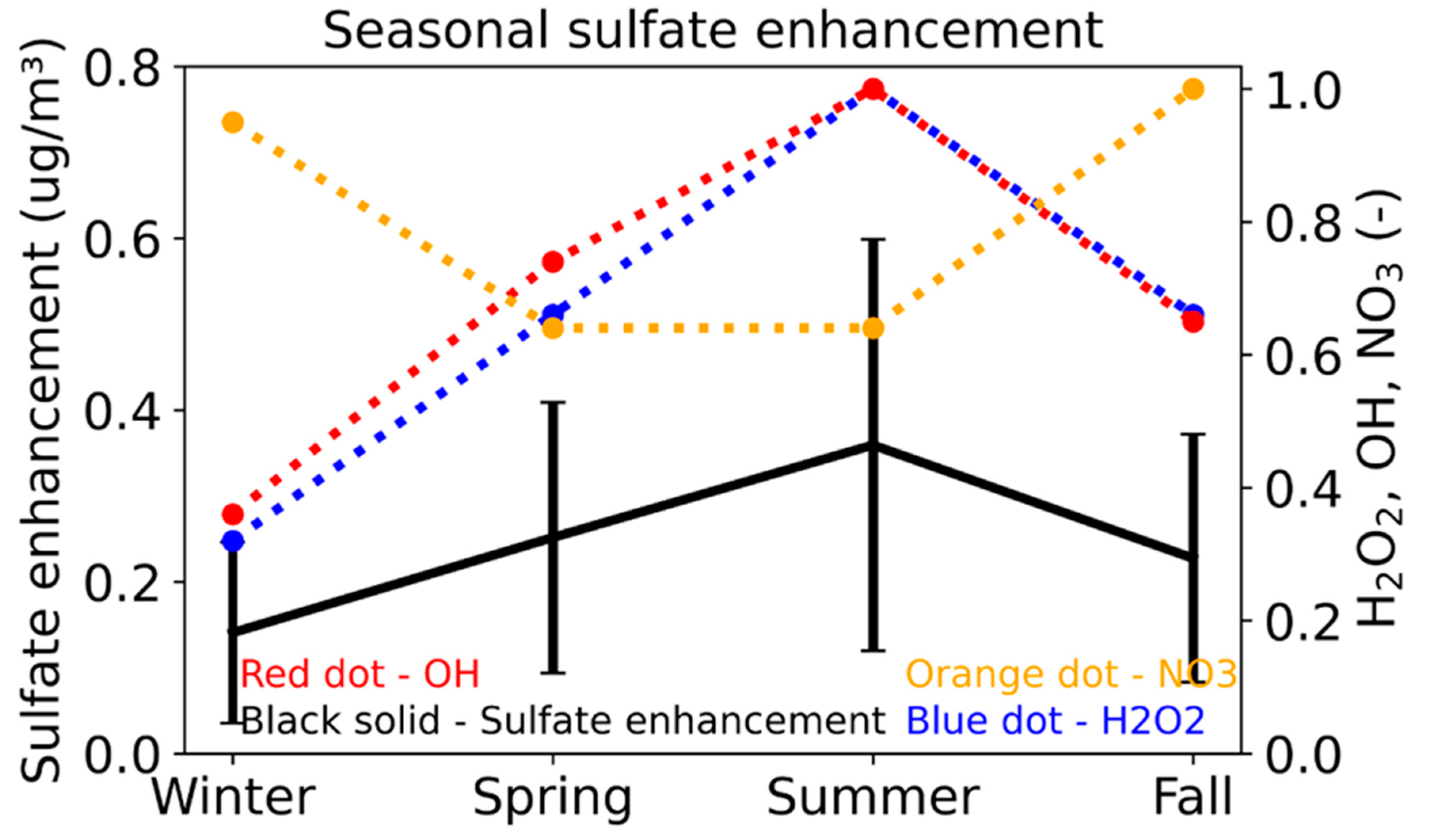
The mean seasonal impacts of DMS emissions on sulfate along with OH, NO3, and H2O2 concentrations over seawater are shown in Figure 3. DMS enhances sulfate in each season, with the greatest enhancement occurring in summer and the smallest in winter. The enhancement in summer is ~2.5 times greater than that in winter, which is consistent with increased emissions and increased oxidation. The formation of sulfate from DMS occurs in two steps. In the first step, DMS is oxidized into SO2 via the OH-, NO3-, and Cl- initiated reactions. DMS oxidation via the Cl-initiated reaction is generally smaller than the other pathways, since Cl levels are lower than other oxidants. In the second step, the resulting SO2 is oxidized into sulfate via the gas-phase reaction with OH and aqueous-phase reactions with H2O2 and other oxidants. Sulfur oxidation by H2O2 in cloud and OH in the gas phase are important processes for producing sulfate in the atmosphere [9]. While NO3 levels are higher in winter and fall, both OH and H2O2 concentrations peak in summer. Thus, both the DMS and SO2 oxidation can occur efficiently, producing the highest sulfate enhancement in summer. In contrast, both OH and H2O2 concentrations are the smallest in winter, producing the lowest enhancement in sulfate.
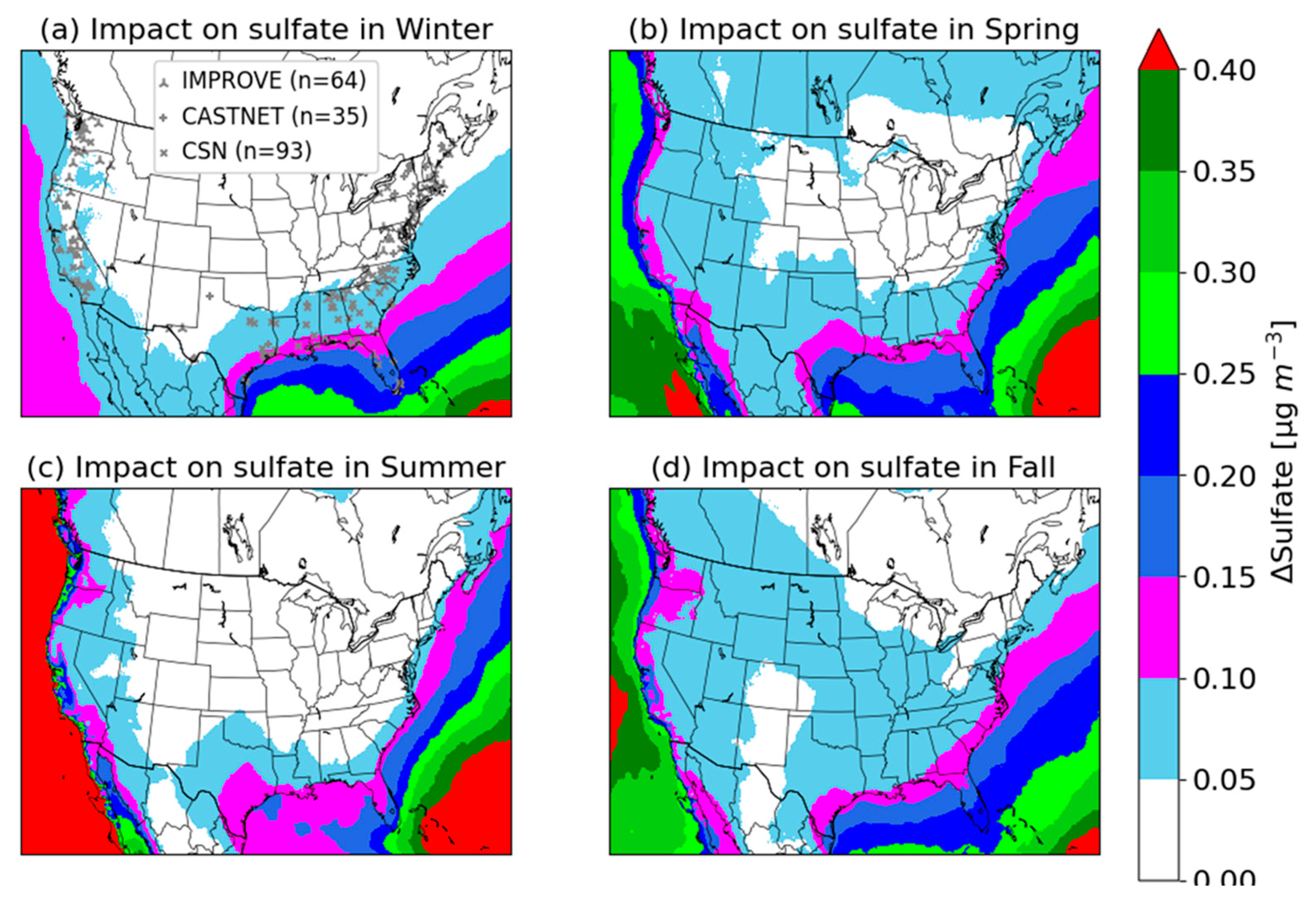
The spatial distribution of the seasonal impacts is shown in Figure 4. Consistent with the annual results shown in Figure 2a, larger impacts occur over seawater than those over land in all seasons. DMS-induced sulfate enhancements are lower in winter over most areas than those in other seasons. In winter, however, DMS emissions increase sulfate over the Gulf of Mexico and part of the Atlantic Ocean by larger margins than those over the Pacific Ocean, leading to higher sulfate concentrations in the winter. In other seasons, DMS increases sulfate over the Pacific Ocean by larger margins due to the contribution from the western boundary condition, higher DMS emissions, and higher oxidant levels. The impacts of DMS emissions over seawater are the highest in summer; however, the impacts tend to be localized over coastal areas. The spatial distributions of the impacts on sulfate are different in spring and fall than those in summer. The mean enhancements over seawater in spring and fall are lower than those in summer. However, DMS emissions produce greater impacts over a large interior portion of land in spring and fall due to higher wind speed, which can effectively transport the resulting sulfate to land. Wind speed is the highest in winter; however, sulfate enhancements are the lowest; thus, the impacts over land are not as widespread as predicted in spring and fall. The average DMS-induced sulfate enhancements over land are 0.04 μg/m3 (6%), 0.07 μg/m3 (8%), 0.05 μg/m3 (11%), and 0.06 μg/m3 (13%) in winter, spring, summer, and fall, respectively.
3.3. Diurnal Variation in the Sulfate Enhancement
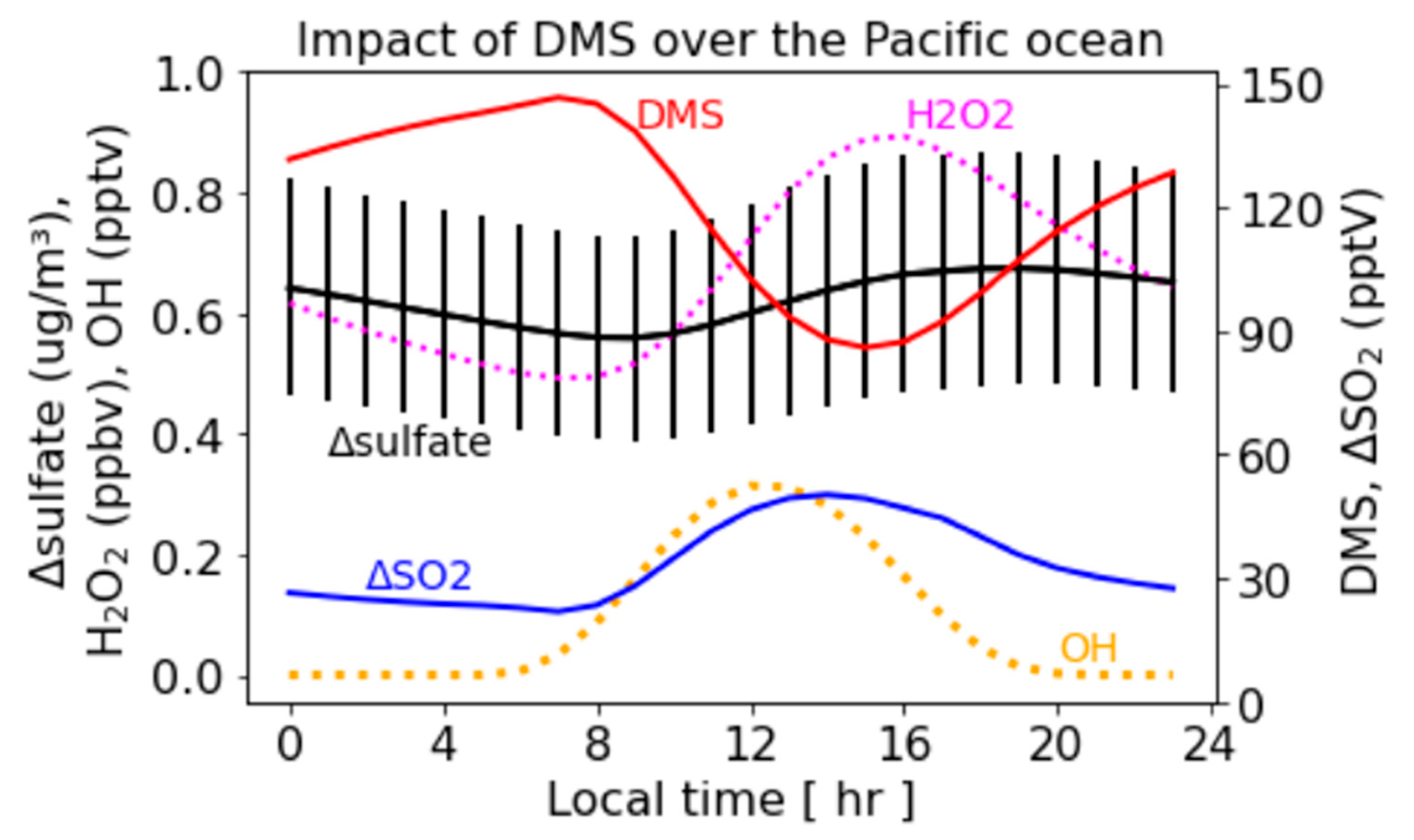
To examine the diurnal variation in DMS-induced sulfate, we selected all grid cells over the Pacific Ocean (including the Gulf of California) in July. The diurnal variation in H2O2, OH, DMS, and SO2 and the sulfate produced by DMS emissions over the Pacific Ocean are shown in Figure 5. OH concentrations remain low at night, start increasing during the day, and peak around noon. H2O2 concentrations are also lower at night, increase during the day, and peak during the mid-afternoon. DMS concentrations slowly increase from midnight to morning, as DMS is continuously emitted but is only oxidized by NO3 at night, which is lower in summer than in winter. The DMS concentrations decrease sharply during the day, reach their lowest level around mid-afternoon, and then increase again. The decrease in DMS concentrations during the day occurs due to higher OH concentrations. SO2 levels remain relatively flat during the night despite SO2 production from the oxidation of DMS by NO3. SO2 concentrations start increasing during the day as more DMS is oxidized by higher daytime OH levels, peak at mid-afternoon, and then decrease at night. Sulfate from the DMS emissions tends to decrease slowly during the night, as little sulfate is produced since OH and H2O2 are lower at night. Sulfate levels increase during the day and peak in the late afternoon due to increased oxidation by OH (in gas phase) and H2O2 in clouds. Thus, DMS-induced sulfate tends to be higher during the day and lower at night.
3.4. Impact of DMS Emissions on Sulfate Aloft
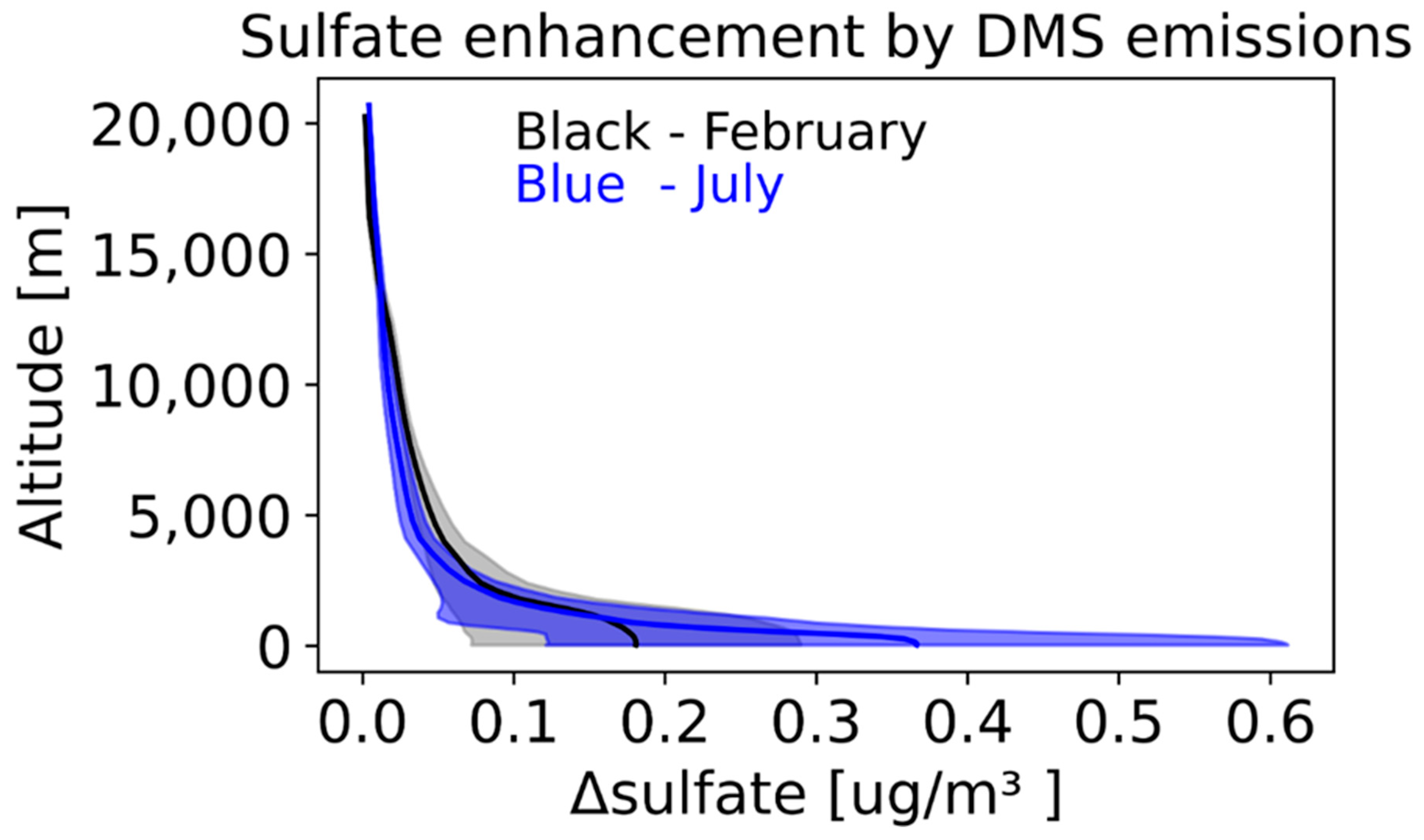
To examine the impact of DMS emissions aloft, we focused on a winter (February) and a summer (July) month. DMS-induced sulfate enhancements over the entire oceanic area with altitude are shown in Figure 6. DMS emissions enhance surface-layer sulfate by ~0.2 μg/m3 in February and ~0.4 μg/m3 in July. These emissions consistently produce more sulfate in summer than in winter. DMS-induced sulfate enhancements are highest at the surface and decrease with altitude, diminishing to ~10–20% at an altitude of ~5 km. Thus, the DMS emissions enhance sulfate not only at the surface layer but also aloft, though its impact tends to be limited in the lower troposphere.
3.5. Impact of DMS Emissions and Boundary Conditions on Sulfate
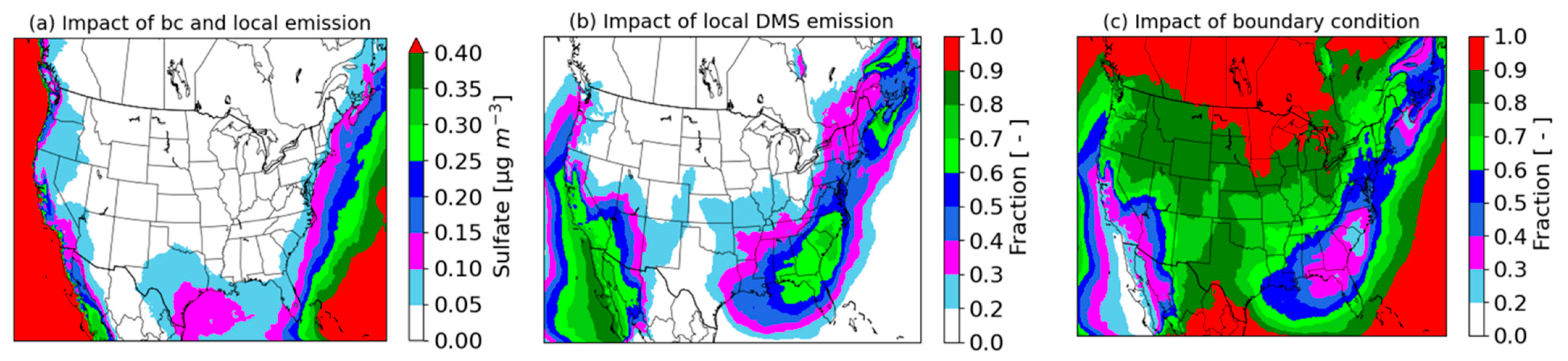
To understand the relative importance of in-domain emissions and transport on sulfate, we completed an additional sensitivity simulation similar to WDMS, but without DMS emissions, in the 12 km domain. The additional sensitivity simulation, therefore, only has DMS and products from the boundary conditions, so we refer to it as BCDMS. The in-domain contribution is calculated as the difference between WDMS (both BC and local emissions) and BCDMS (only BC). The boundary contribution is calculated as the difference between BCDMS (only BC) and NODMS (no DMS). The combined impacts of in-domain DMS emissions and boundary conditions (WDMS—NODMS) on July mean sulfate are shown in Figure 7a. Consistent with Figure 2a and Figure 4c, DMS emissions and boundary conditions produce higher impacts over seawater than over land, and they also enhance sulfate in many coastal areas. Figure 7b,c show the fractional contributions of in-domain DMS emissions (WDMS—BCDMS) and outside-domain DMS emissions (BCDMS—NODMS) to the total sulfate enhancement (WDMS—NODMS) shown in Figure 7a. In-domain DMS emissions increase sulfate over seawater by fractions of >0.6 over the southern Pacific coast, the southern Atlantic coast, and the coast of Maine (Figure 7b). In contrast, boundary conditions enhance sulfate over seawater by fractions of >0.6 over the northern Pacific coast, further offshore in the Atlantic/Gulf of Mexico, the tip of Florida, and over a large land area (Figure 7c). While the combined impacts of DMS emissions and boundary conditions over the interior portion of the modeling domain are relatively small (<0.05 μg/m3), the impact over this region is dominated by boundary conditions, i.e., the long-range transport of sulfate formed from DMS emissions over the hemisphere. These results suggest that boundary conditions play an important role on sulfate enhancements not only near the boundaries but also over the interior portion of the modeling domain. Thus, it is important to employ appropriate boundary conditions in the model; otherwise, regional-scale model predictions will not reflect the full effects of DMS emissions on the relevant temporal and spatial scales. It should be noted that boundary conditions obtained with the DMS emissions from the hemispheric model include the impacts on DMS, SO2, and sulfate. These results suggest that enhancements in sulfate from DMS on the Pacific Northwest of 0.25–0.3 μg/m3 are primarily from emissions outside the domain. This is consistent with large fluxes between the Pacific Northwest and Alaska from May through August, as evident in Zhao et al. [20] and Hulswar et al. [58].
3.6. Comparison with Observed Sulfate
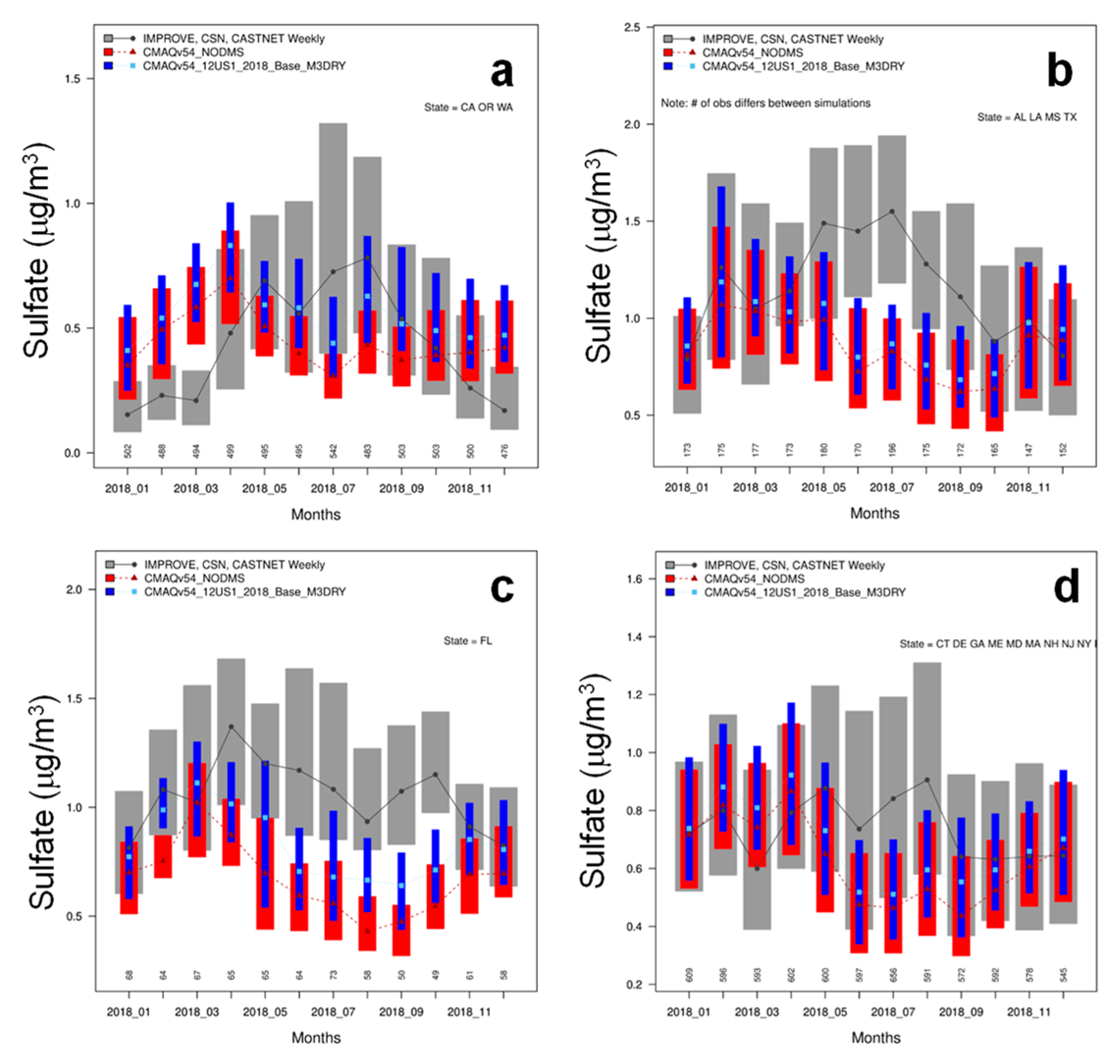
The largest impact of DMS emissions on land occurs in coastal areas. Thus, we focused on model performance in coastal states and compared model predictions with observed data in four separate groups: (1) the Pacific Coast states (Washington, Oregon, California), (2) the Gulf Coast states (Texas, Louisiana, Mississippi, Alabama), (3) Florida, and (4) the Atlantic Coast states (Georgia, South Carolina, North Carolina, Virginia, Maryland, Delaware, New Jersey, New York, Connecticut, Rhode Island, Massachusetts, New Hampshire, Maine). We calculated the monthly mean observed sulfate concentrations by combining data from IMPROVE (Interagency Monitoring of Protected Visual Environments), CASTNET (Clean Air Status and Trends Network), and CSN (Chemical Speciation Network) sites within each group. We then calculated the mean sulfate concentrations without and with DMS emissions by combining predictions at all sites within the group and compared them to the corresponding observed data.
Figure 8 shows that the effect on performance varies by region and season. In all regions, the NODMS underpredicts May through October observations. Adding DMS improves the model performance. For the cooler months, the performance is mixed because the base model overpredicts in some places and underpredicts in others. For cooler months (January–April, November, December), NODMS overpredicts compared to observations, so adding DMS deteriorates the model performance. In the Gulf Coast states, NODMS only overpredicts in January and December, and DMS emissions improve the comparison with observed data in all other months. A similar pattern is also noticeable in Florida and the Atlantic Coast states. Thus, additional sulfate from DMS emissions tends to deteriorate the model performance in cooler months while improving it in warmer months.
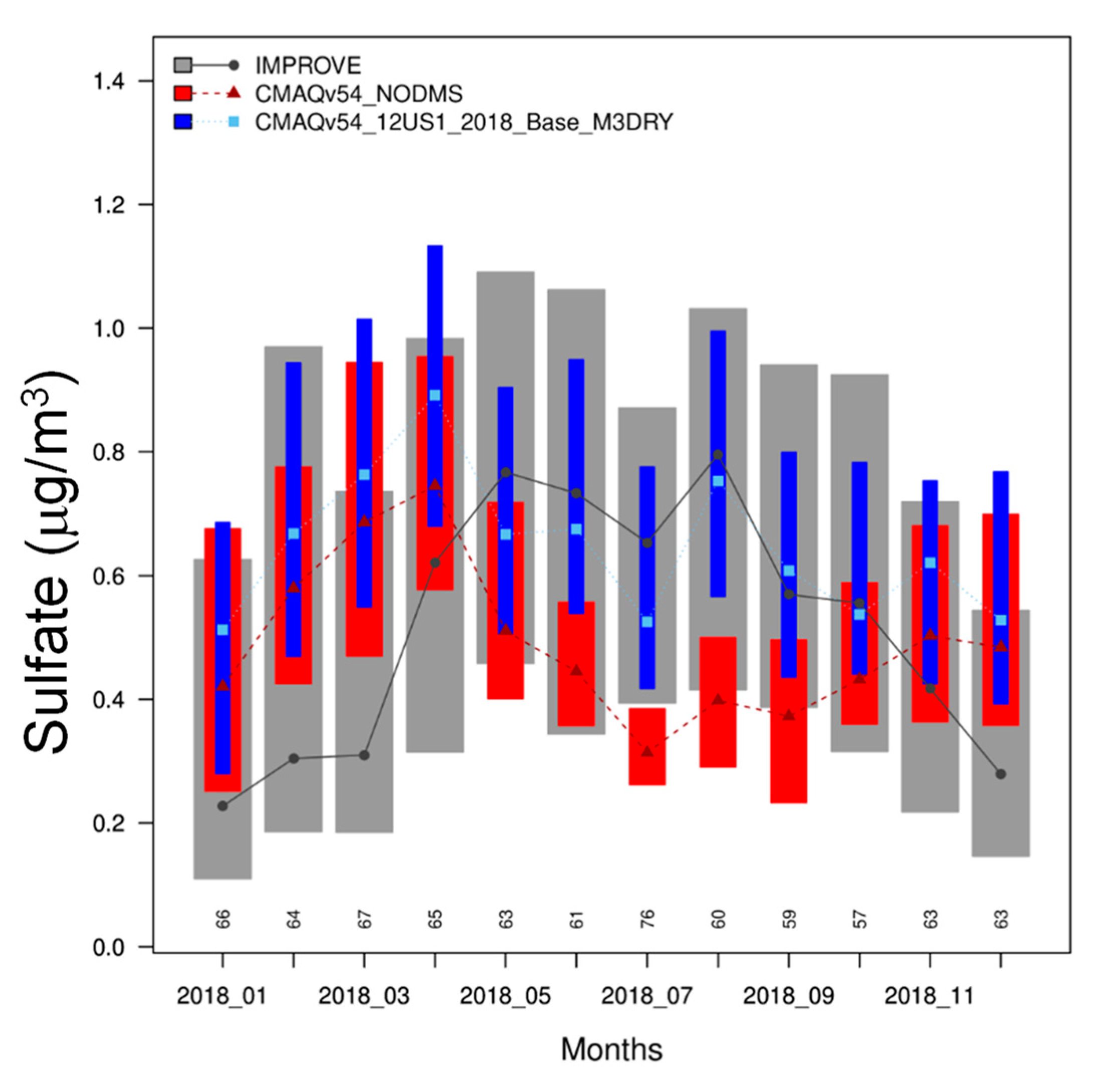
To further examine the impact on model performance, we isolated IMPROVE sites located within 10 km from the coastline in the Pacific Coast states and Florida and compared monthly mean sulfate concentrations without and with DMS emissions to observed data (Figure 9). Similar to Figure 8, DMS emissions deteriorate the model performance in cooler months. However, they improve the comparison in warmer months by larger margins than those shown in Figure 8. Thus, DMS emissions can improve the model performance by a larger margin near the coastal areas than the interior areas.
3.7. Changes in DMS-Initiated Sulfate Enhancement with Horizontal Grid Resolution
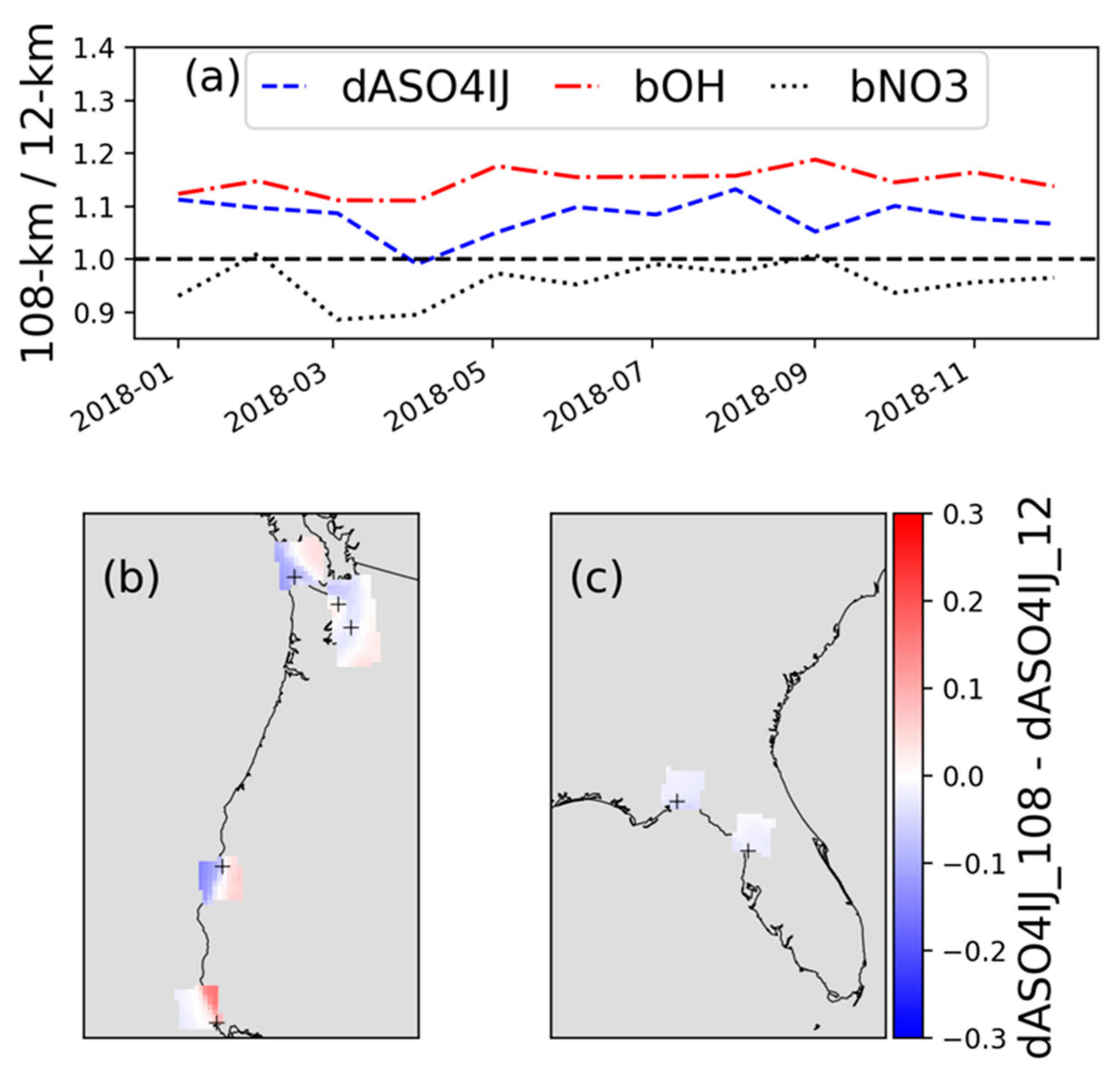
Most of the prior studies employed large-scale models using coarse horizontal grid resolution to examine the impact of oceanic DMS emissions on sulfate. In this study, we used a finer horizontal grid resolution (12 km) over the continental U.S. We also conducted CMAQ simulations without and with DMS emissions over the northern hemisphere using coarse (108 km) horizontal grids, from which we created boundary conditions for model simulations over the continental U.S. Here, we examined the impacts of DMS emissions on sulfate using results from simulations obtained with 12 km and 108 km horizontal grids. We calculated DMS-initiated monthly mean sulfate enhancements over the entire seawater of the modeling domain covering the continental U.S. using both the 108 km and 12 km horizontal grids. Over the entire seawater, ratios of sulfate enhancements with 108 km grids to 12 km horizontal grids are greater than 1.0 (Figure 10a), which indicates that model with 108 km grids produces slightly more DMS-initiated sulfate than the model with 12 km grids. Ratios of model OH and NO3 concentrations over the seawater with 108 km and 12 km grids are also shown in Figure 10a. The OH concentrations over the entire seawater are consistently greater with 108 km grids than those with 12 km grids (ratio > 1.0). In contrast, the NO3 concentrations over the entire seawater are generally lower with 108 km grids than those with 12 km grids (ratio < 1.0). The grid resolution affects many parameters in the model which, in turn, affect DMS-initiated sulfate enhancements. However, OH appears to play an important role in affecting the DMS-initiated sulfate enhancement. The higher DMS-initiated sulfate with 108 km grids occurs primarily due to additional DMS oxidation via higher OH concentrations and additional SO2 oxidation with OH concentrations. However, such enhancements with 108 km grids do not occur in all areas. For example, the model with 108 km grids generally produces more sulfate enhancements over the Pacific Ocean. In contrast, the model with 108 km grids produces less sulfate enhancements over portions of the Gulf of Mexico and the Atlantic Ocean, primarily due to reduced DMS oxidation by lower NO3 concentrations and reduced SO2 oxidation by lower H2O2 concentrations. Thus, DMS-initiated sulfate enhancements are dependent on grid resolution and geographic location. To further illustrate the complexity of evaluating the impacts of grid resolution at individual sites, the annual mean difference in DMS-initiated sulfate at the seven coastal IMPROVE sites (same sites used in Figure 9) are shown in Figure 10b,c. Each 108 km grid cell contains 81 approximately 12 km grid cells. The model with 108 km grids produces lower sulfate enhancements consistently at the two sites in Florida than those with the model with 12 km grids. However, the impacts at the western U.S. sites are mixed within 108 km grid cells. The model with 108 km grids produces more sulfate enhancements at some sites while producing less sulfate enhancements at other sites. Such results show the importance of considering grid resolution in evaluating the impacts of DMS-initiated sulfate enhancements.
4. Conclusions
We examined the impacts of DMS emissions on sulfate concentrations over the continental U.S. and surrounding areas by using CMAQv5.4 with a horizontal grid resolution of 12 km and boundary conditions derived from a comparable hemispheric-scale model. DMS emissions increase annual mean sulfate concentrations over seawater and land areas, with the largest impact over seawater. In-domain DMS emissions increase sulfate more over coastal areas than over interior portions of land, with the largest impacts occurring over Washington, Oregon, California, and Florida. Seasonally, the largest enhancements over seawater occur in summer and the lowest in winter. These enhancements help reduce the low bias in modeled sulfate at coastal sites in California, Washington, and Florida. The over-seawater enhancements in spring and fall are lower than those in summer but greater than those in winter. However, enhanced sulfate can occur deeper into land areas in spring and fall due to the prevailing higher wind speeds, causing slightly higher enhancements than those in summer. DMS emissions increase sulfate throughout the lower troposphere, though the impacts at higher altitudes decrease sharply compared to those near the surface. Predicted sulfate with DMS deteriorates the model performance in cooler months, while improving it in warmer months. DMS plays a larger role in affecting the model performance in coastal areas. Sulfate enhancements from DMS emissions on a hemispheric scale represented through boundary conditions for the 12 km domain play an important role in affecting sulfate enhancements, not only near the boundaries, but also in the interior portion of the modeling domain.
As indicated by our results, the oxidation of DMS in the troposphere and subsequent conversion to SO2 are key processes for the formation and growth in sulfur-containing aerosols in the marine boundary layer, which then can also undergo long-range transport and influence background aerosol sulfate levels in continental areas. Though our current implementation of DMS chemistry captures the dominant oxidation pathways via OH and NO3, future enhancements in the representation of halogen chemistry in the model enable a more complete representation of DMS oxidation by reactive halogens as well as multi-phase pathways [16]. Additionally, Veres et al. [59] recently identified hydroperoxymethyl thioformate (HPMTF) as a new DMS oxidation product in measurements performed during the Atmospheric Tomography mission over marine environments. The addition of HPMTF and its oxidation pathways could potentially slow down DMS oxidation to SO2 and thus reduce the abundance of SO2 and sulfate in areas of DMS emissions but enhance their levels in downwind cloud-free regions where HPTMF can continue to oxidize to produce SO2 and sulfate. In contrast, Novak et al. [60] suggest that in the cloudy marine boundary layer, the HPMTF lifetime is considerably reduced due to uptake in cloud droplets, limiting the production of SO2. However, the paucity of direct observations of the full suite of DMS oxidation products across the variable conditions of the marine boundary layer make it challenging to adequately constrain the reaction pathways and SO2 yields from DMS oxidation. Future efforts will focus on enhancing the representation of these pathways, as better estimates of these multiphase chemical pathways evolve.
Author Contributions
Conceptualization, G.S.; methodology, G.S.; software, G.S., C.H., W.A. and B.H.H.; validation, G.S., W.A. and B.H.H.; formal analysis, G.S. and B.H.H.; investigation, G.S. and B.H.H.; data curation, G.S., B.H.H., C.H. and W.A.; writing—original draft preparation, G.S., D.K. and B.H.H.; writing—review and editing, G.S., D.K., W.A., C.H., B.H.H. and R.M.; visualization, G.S. and B.H.H.; project administration, G.S. All authors have read and agreed to the published version of the manuscript.
Funding
This research received no external funding.
Institutional Review Board Statement
The views expressed in this paper are those of the authors and do not necessarily represent the views or policies of the U.S. EPA. Mention of trade names or commercial products does not con-stitute endorsement or recommendation for use.
Informed Consent Statement
Not applicable.
Data Availability Statement
Data will be made available on request.
Acknowledgments
We thank David Olson and Ivan R. Piletic of EPA for performing internal reviews of the article.
Conflicts of Interest
The authors declare no conflict of interest.
References
- Carpenter, L.J.; Archer, S.D.; Beale, R. Ocean-atmosphere trace gas exchange. Chem. Soc. Rev. 2012, 41, 6473–6506. [Google Scholar] [CrossRef] [PubMed]
- Charlson, R.J.; Lovelock, J.E.; Andreae, M.O.; Warren, S.G. Oceanic phytoplankton, atmospheric sulphur, cloud albedo and climate. Nature 1987, 326, 655–661. [Google Scholar] [CrossRef]
- Lana, A.; Bell, T.G.; Simó, R.; Vallina, S.M.; Ballabrera-Poy, J.; Kettle, A.J.; Dachs, J.; Bopp, L.; Saltzman, E.S.; Stefels, J.; et al. An updated climatology of surface dimethlysulfide concentrations and emission fluxes in the global ocean. Glob. Biogeochem. Cycles 2011, 25. [Google Scholar] [CrossRef] [Green Version]
- Fung, K.M.; Heald, C.L.; Kroll, J.H.; Wang, S.; Jo, D.S.; Gettelman, A.; Lu, Z.; Liu, X.; Zaveri, R.A.; Apel, E.C.; et al. Exploring dimethyl sulfide (DMS) oxidation and implications for global aerosol radiative forcing. Atmos. Chem. Phys. 2022, 22, 1549–1573. [Google Scholar] [CrossRef]
- Aas, W.; Mortier, A.; Bowersox, V.; Cherian, R.; Faluvegi, G.; Fagerli, H.; Hand, J.; Klimont, Z.; Galy-Lacaux, C.; Lehmann, C.M.B.; et al. Global and regional trends of atmospheric sulfur. Nat. Sci. Rep. 2019, 9, 953. [Google Scholar] [CrossRef] [Green Version]
- Tanner, R.L.; Bairai, S.T.; Mueller, S.F. Trends in concentrations of atmospheric gaseous and particulate species in rural eastern Tennessee as related to primary emission reductions. Atmos. Chem. Phys. 2015, 15, 9781–9797. [Google Scholar] [CrossRef] [Green Version]
- Malm, W.C.; Schichtel, B.A.; Hand, J.L.; Collett, J.L., Jr. Concurrent temporal and spatial trends in sulfate and organic mass concentrations measured in the IMPROVE Monitoring Program. J. Geophys. Res. Atmos. 2017, 122, 10462–10476. [Google Scholar] [CrossRef]
- Avise, J.; Chen, J.; Turkiewicz, K.; DaMassa, J.; Vanderspek, S. Wintertime PM2.5 Pollution in California, EM, The Magazine for Environmental Managers, A&WMA, December 2019. Available online: www.awma.org/em/ (accessed on 23 January 2023).
- Seinfeld, J.H.; Pandis, S.N. Atmospheric Chemistry and Physics: From air pollution to Climate Change; John Wiley & Sons: Hoboken, NJ, USA, 2006. [Google Scholar]
- Lee, C.L.; Brimblecombe, P. Anthropogenic contributions to global carbonyl sulfide, carbon disulfide and organosulfides fluxes. Earth-Sci. Rev. 2016, 160, 1–18. [Google Scholar] [CrossRef] [Green Version]
- Boucher, O.; Randall, D.; Artaxo, P.; Bretherton, C.; Feingold, G.; Forster, P.; Kerminen, V.-M.; Kondo, Y.; Liao, H.; Lohmann, U. Clouds and Aerosols, Climate Change 2013: The Physical Science Basis. Contribution of Working Group I to the Fifth Assessment Report of the Intergovernmental Panel on Climate Change; Cambridge University Press: Cambridge, UK, 2013; pp. 571–657. [Google Scholar] [CrossRef]
- Breider, T.J.; Chipperfield, M.P.; Richards, N.A.D.; Carslaw, K.S.; Mann, G.W.; Spracklen, D.V. Impact of BrO on dimethylsulfide in the remote marine boundary layer. Geophys. Res. Lett. 2010, 37, L02807. [Google Scholar] [CrossRef]
- Park, R.J.; Jacob, D.J.; Field, B.D.; Yantosca, R.M.; Chin, M. Natural and transboundary pollution influences on sulfate-nitrate-ammonium aerosols in the United States: Implications for policy. J. Geophys. Res.-Atmos. 2004, 109, D15204. [Google Scholar] [CrossRef]
- Kloster, S.; Feichter, J.; Maier-Reimer, E.; Six, K.D.; Stier, P.; Wetzel, P. DMS cycle in the marine ocean-atmosphere system; a global model study. Biogeosciences 2006, 3, 29–51. [Google Scholar] [CrossRef] [Green Version]
- Thomas, M.A.; Suntharalingam, P.; Pozzoli, L.; Rast, S.; Devasthale, A.; Kloster, S.; Feichter, J.; Lenton, T.M. Quantification of DMS aerosol-cloud-climate interactions using the ECHAM5-HAMMOZ model in a current climate scenario. Atmos. Chem. Phys. 2010, 10, 7425–7438. [Google Scholar] [CrossRef] [Green Version]
- Chen, Q.; Sherwen, T.; Evans, M.; Alexander, B. DMS oxidation and sulfur aerosol formation in the marine troposphere: A focus on reactive halogen and multiphase chemistry. Atmos. Chem. Phys. 2018, 18, 13617–13637. [Google Scholar] [CrossRef] [Green Version]
- Itahashi, S.; Mathur, R.; Hogrefe, C.; Napelenok, S.L.; Zhang, Y. Incorporation of volcanic SO2 emissions in the Hemispheric CMAQ (H-CMAQ) version 5.2 modeling system and assessing their impacts on sulfate aerosol over the Northern Hemisphere. Geosci. Model Dev. 2021, 14, 5751–5768. [Google Scholar] [CrossRef] [PubMed]
- Mueller, S.F.; Mao, Q.; Mallard, J.W. Modeling natural emissions in the Community Multiscale Air Quality (CMAQ) model—Part 2: Modifications for simulating natural emissions. Atmos. Chem. Phys. 2011, 11, 293–320. [Google Scholar] [CrossRef] [Green Version]
- Perraud, V.; Horne, J.R.; Martinez, A.S.; Kalinowski, J.; Meinardi, S.; Dawson, M.L.; Wingen, L.M.; Dabdub, D.; Blake, D.R.; Gerber, R.B.; et al. The future of airborne sulfur-containing particles in the absence of fossil fuel sulfur dioxide emissions. Proc. Natl. Acad. Sci. USA 2015, 112, 13514–13519. [Google Scholar] [CrossRef] [Green Version]
- Zhao, J.; Sarwar, G.; Gantt, B.; Foley, K.; Henderson, B.H.; Pye, H.O.T.; Fahey, K.M.; Kang, D.; Mathur, R.; Zhang, Y.; et al. Impact of dimethylsulfide chemistry on air quality over the Northern Hemisphere. Atmos. Environ. 2021, 244, 117961. [Google Scholar] [CrossRef]
- Appel, K.W.; Bash, J.O.; Fahey, K.M.; Foley, K.M.; Gilliam, R.C.; Hogrefe, C.; Hutzell, W.T.; Kang, D.; Mathur, R.; Murphy, B.N.; et al. The Community Multiscale Air Quality (CMAQ) model versions 5.3 and 5.3.1: System updates and evaluation. Geosci. Model Dev. 2021, 14, 2867–2897. [Google Scholar] [CrossRef]
- Kitayama, K.; Morino, Y.; Yamaji, K.; Chatani, S. Uncertainties in O3 concentrations simulated by CMAQ over Japan using four chemical mechanisms. Atmos. Environ. 2019, 198, 448–462. [Google Scholar] [CrossRef]
- East, J.D.; Henderson, B.H.; Napelenok, S.L.; Koplitz, S.N.; Sarwar, G.; Gilliam, R.; Lenzen, A.; Tong, D.Q.; Pierce, R.B.; Garcia-Menendez, F. Inferring and evaluating satellite-based constraints on NOx emissions estimates in air quality simulations. Atmos. Chem. Phys. Discuss. 2022. in review. [Google Scholar] [CrossRef]
- Mathur, R.; Kang, D.; Napelenok, S.L.; Xing, J.; Hogrefe, C.; Sarwar, G.; Itahashi, S.; Henderson, B.H. How have divergent global emission trends influenced long-range transported ozone to North America? J. Geophys. Res. Atmos. 2022, 127, e2022JD036926. [Google Scholar] [CrossRef]
- Sarwar, G.; Christian Hogrefe, H.; Henderson, B.H.; Foley, K.; Mathur, R.; Murphy, B.; Ahmed, S. 2023 Characterizing variations in ambient PM25 concentrations at the, U.S. Embassy in Dhaka, Bangladesh using observations and the CMAQ modeling system. Atmos. Environ. 2023, 296, 119587. [Google Scholar] [CrossRef]
- US Environmental Protection Agency, 2022. CMAQ (Version 5.4) [Software]. Available online: https://zenodo.org/record/7218076#.ZCZVRHZBxPY (accessed on 25 March 2023).
- Skamarock, W.C.; Klemp, J.B. A time-split nonhydrostatic atmospheric model for weather research and forecasting applications. J. Comput. Phys. 2008, 227, 3465–3485. [Google Scholar] [CrossRef]
- Iacono, M.J.; Delamere, J.S.; Mlawer, E.J.; Shephard, M.W.; Clough, S.A.; Collins, W.D. Radiative forcing by long-lived greenhouse gases: Calculations with the AER radiative transfer models. J. Geophys. Res. Atmos. 2008, 113. [Google Scholar] [CrossRef]
- Kain, J.S. The Kain-Fritsch Convective Parameterization: An Update. J. Appl. Meteorol. 2004, 43, 170–181. [Google Scholar] [CrossRef]
- Heath, N.K.; Pleim, J.E.; Gilliam, R.C.; Kang, D. A simple lightning assimilation technique for improving retrospective WRF simulations. J. Adv. Model. Earth Syst. 2016, 8, 1806–1824. [Google Scholar] [CrossRef] [PubMed]
- Kang, D.; Heath, N.K.; Gilliam, R.C.; Spero, T.L.; Pleim, J.E. Lightning assimilation in the WRF model (Version 4.1.1): Technique updates and assessment of the applications from regional to hemispheric scales. Geosci. Model Dev. 2022, 15, 8561–8579. [Google Scholar] [CrossRef]
- Morrison, H.; Gettelman, A. A new two-moment bulk stratiform cloud microphysics scheme in the Community Atmosphere Model, version 3 (CAM3). Part I: Description and numerical tests. J. Clim. 2008, 21, 3642–3659. [Google Scholar] [CrossRef]
- Pleim, J.E.; Xiu, A. Development and testing of a surface flux and planetary boundary layer model for application in mesoscale models. J. Appl. Meteorol. 1995, 34, 16–32. [Google Scholar] [CrossRef] [Green Version]
- Xiu, A.; Pleim, J.E. Development of a land surface model. Part I: Application in a mesoscale meteorological model. J. Appl. Meteorol. 2001, 40, 192–209. [Google Scholar] [CrossRef]
- Pleim, J.E. A combined local and nonlocal closure model for the atmospheric boundary layer. Part I: Model description and testing. J. Appl. Meteorol. Climatol. 2007, 46, 1383–1395. [Google Scholar] [CrossRef]
- Pleim, J.E. A combined local and nonlocal closure model for the atmospheric boundary layer. Part II: Application and evaluation in a mesoscale meteorological model. J. Appl. Meteorol. Climatol. 2007, 46, 1396–1409. [Google Scholar] [CrossRef] [Green Version]
- Gilliam, R.C.; Godowitch, J.M.; Rao, S.T. Improving the Horizontal Transport in the Lower Troposphere with Four Dimensional Data Assimilation (Vol. 53). Atmos. Environ. 2012, 53, 186–201. [Google Scholar] [CrossRef]
- Otte, T.L.; Pleim, J.E. The Meteorology-Chemistry Interface Processor (MCIP) for the CMAQ modeling system: Updates through MCIPv3.4.1. Geosci. Model Dev. 2010, 3, 243–256. [Google Scholar] [CrossRef] [Green Version]
- Torres-Vazquez, A.; Pleim, J.; Gilliam, R.; Pouliot, G. Performance evaluation of the meteorology and air quality conditions from multiscale WRF-CMAQ simulations for the Long Island Sound Tropospheric Ozone Study (LISTOS). J. Geophys. Res. Atmos. 2022, 127, e2021JD035890. [Google Scholar] [CrossRef] [PubMed]
- Yarwood, G.; Shi, Y.; Beardsley, R. Impact of CB6r5 Mechanism Changes on Air Pollutant Modeling in Texas. Final Report prepared for Texas Commission on Environmental Quality, Austin, TX 78753, USA; Ramboll US Corporation: Novato, CA, USA, 2020. [Google Scholar]
- Sarwar, G.; Simon, H.; Bhave, P.; Yarwood, G. Examining the impact of heterogeneous nitryl chloride production on air quality across the United States. Atmos. Chem. Phys. 2012, 12, 6455–6473. [Google Scholar] [CrossRef] [Green Version]
- EPA, 2021. 2017 National Emissions Inventory: January 2021 Updated Release, Technical Support Document, U.S. Environmental Protection Agency, Office of Air Quality Planning and Standards Air Quality Assessment Division, Emissions Inventory and Analysis Group, Research Triangle Park, NC, EPA-454/R-21-001, February 2021. Available online: https://www.epa.gov/sites/default/files/2021-02/documents/nei2017_tsd_full_jan2021.pdf (accessed on 2 March 2022).
- Gantt, B.; Kelly, J.T.; Bash, J.O. Updating sea spray aerosol emissions in the Community Multiscale Air Quality (CMAQ) Model Version 5.0.2. Geosci. Model Dev. 2015, 8, 3733–3746. Available online: www.geosci-model-dev.net/8/3733/2015/ (accessed on 15 March 2022). [CrossRef] [Green Version]
- Kang, D.; Pickering, K.E.; Allen, D.J.; Foley, K.M.; Wong, D.C.; Mathur, R.; Roselle, S.J. Simulating lightning NO production in CMAQv5.2: Evolution of scientific updates. Geosci. Model Dev. 2019, 12, 3071–3083. [Google Scholar] [CrossRef] [Green Version]
- Kettle, A.J.; Andreae, M.O.; Amouroux, D.; Andreae, T.W.; Bates, T.S.; Berresheim, H.; Bingemer, H.; Boniforti, R.; Curran, M.A.J.; DiTullio, G.R.; et al. A global database of sea surface dimethylsulfide (DMS) measurements and a procedure to predict sea surface DMS as a function of latitude, longitude, and month. Glob. Biogeochem. Cycles 1999, 13, 399–444. [Google Scholar] [CrossRef]
- Kettle, A.J.; Andreae, M.O. Flux of dimethylsulfide from the oceans: A comparison of updated data sets and flux models. J. Geophys. Res. Atmos. 2000, 105, 26793–26808. [Google Scholar] [CrossRef]
- Liss, P.S.; Merlivat, L. Air-Sea Gas Exchange Rates: Introduction and Synthesis. In The Role of Air-Sea Exchange in Geochemical Cycling; Buat-Ménard, P., Ed.; Springer: Dordrecht, The Netherlands, 1986; pp. 113–127. [Google Scholar]
- Nightingale, P.D.; Malin, G.; Law, C.S.; Watson, A.J.; Liss, P.S.; Liddicoat, M.I.; Boutin, J. Upstill-Goddard, R.C. In situ evaluation of air-sea gas exchange parameterizations using novel conservative and volatile tracers. Glob. Biogeochem. Cycles 2000, 14, 373–387. [Google Scholar] [CrossRef]
- Wanninkhof, R. Relationship between wind speed and gas exchange over the ocean. J. Geophys. Res. Ocean. 1992, 97, 7373–7382. [Google Scholar] [CrossRef]
- Saltzman, E.S.; King, D.B.; Holmen, K.; Leck, C. Experimental determination of the diffusion coefficient of dimethyl sulfide in water. J. Geophys. Res. Oceans 1993, 98, 16481–16486. [Google Scholar] [CrossRef] [Green Version]
- McGillis, W.R.; Dacey, J.; Frew, N.M.; Bock, E.J.; Nelson, R.K. Water-air flux of dimethylsulfide. J. Geophys. Res. Oceans 2000, 105, 1187–1193. [Google Scholar] [CrossRef]
- Smith, S.N.; Mueller, S.F. Modeling natural emissions in the Community Multiscale Air Quality (CMAQ) Model–I: Building an Emissions Data Base. Atmos. Chem. Phys. 2010, 10, 4931–4952. [Google Scholar] [CrossRef] [Green Version]
- Sander, S.; Friedl, R.; Abbatt, J.; Barker, J.; Burkholder, J.; Golden, D.; Kolb, C.; Kurylo, M.; Moortgat, G.; Wine, P.J.J. Chemical kinetics and photochemical data for use in atmospheric studies, evaluation number. JPL 2011, 14, 10. [Google Scholar]
- Atkinson, R.; Cox, R.A.; Crowley, J.N.; Hampson, R.F.; Hynes, R.G.; Jenkin, M.E.; Kerr, J.A.; Rossi, M.J.; Troe, J. Summary of Evaluated Kinetic and Photo-Chemical Data for Atmospheric Chemistry; Technical Report; IUPAC Subcommittee on Gas Kinetic Data Evaluation for Atmospheric Chemistry: October 2006. Available online: http://www.iupac-kinetic.ch.cam.ac.uk/ (accessed on 27 December 2019).
- Sommariva, R.; von Glasow, R. Multiphase Halogen Chemistry in the Tropical Atlantic Ocean. Environ. Sci. Technol. 2012, 46, 10429–10437. [Google Scholar] [CrossRef]
- Mathur, R.; Xing, J.; Gilliam, R.; Sarwar, G.; Hogrefe, C.; Pleim, J.; Pouliot, G.; Roselle, S.; Spero, T.L.; Wong, D.C.; et al. Extending the Community Multiscale Air Quality (CMAQ) modeling system to hemispheric scales: Overview of process considerations and initial applications. Atmos. Chem. Phys. 2017, 17, 12449–12474. [Google Scholar] [CrossRef] [Green Version]
- Lelieveld, J.; Roelofs, G.-J.; Ganzeveld, L.; Feichter, J.; Rodhe, H. Terrestrial sources and distribution of atmospheric sulphur. Philos. Trans. R. Soc. London. Ser. B Biol. Sci. 1997, 352, 149–158. [Google Scholar] [CrossRef]
- Hulswar, S.; Simó, R.; Galí, M.; Bell, T.G.; Lana, A.; Inamdar, S.; Halloran, P.R.; Manville, G.; Mahajan, A.S. Third revision of the global surface seawater dimethyl sulfide climatology (DMS-Rev3). Earth Syst. Sci. Data 2022, 14, 2963–2987. [Google Scholar] [CrossRef]
- Veres, P.R.; Neuman, J.A.; Bertram, T.H.; Assaf, E.; Wolfe, G.M.; Williamson, C.J.; Weinzierl, B.; Tilmes, S.; Thompson, C.R.; Thames, A.B.; et al. Global airborne sampling reveals a previously unobserved dimethyl sulfide oxidation mechanism in the marine atmosphere. Proc. Natl. Acad. Sci. USA 2020, 117, 4505. [Google Scholar] [CrossRef] [PubMed]
- Novak, G.A.; Fite, C.H.; Holmes, C.D.; Veres, P.R.; Neuman, J.A.; Faloona, I.; Thornton, J.A.; Wolfe, G.M.; Vermeuel, M.P.; Jernigan, C.M.; et al. Rapid cloud removal of dimethyl sulfide oxidation products limits SO2 and cloud condensation nuclei production in the marine atmosphere. Proc. Natl. Acad. Sci. USA 2021, 118, e2110472118. [Google Scholar] [CrossRef] [PubMed]
Figure 1.
Seasonal DMS emissions over the modeling domain calculated using the Liss and Merlivat [47] parameterization for the water side gas transfer velocity (). DMSw, wind speed, and SST values shown on the right y-axis are dimensionless. Normalized values were calculated by dividing the actual values by their maximum values. Winter represents December–February, spring represents March–May, summer represents June–August, and fall represents September–November.

Figure 2.
Predicted annual mean changes (WDMS—NODMS) in surface (a) sulfate, (b) nitrate, (c) ammonium, and (d) total inorganic particle concentrations by DMS emissions. Changes in inorganic particle concentrations are calculated as the net effect due to increases in sulfate and ammonium and decreases in nitrate concentrations.

Figure 3.
Seasonal impacts of DMS emissions on sulfate over seawater. H2O2, OH, and NO3 concentrations shown on the right y-axis are dimensionless. Normalized values were calculated by dividing the actual concentrations by their maximum concentrations and are shown on y-axis. Winter represents December–February, spring represents March–May, summer represents June–August, and fall represents September–November. Solid vertical lines represent standard deviation of sulfate enhancement.

Figure 4.
Spatial distribution of the seasonal impacts of DMS emissions on sulfate in (a) winter, (b) spring, (c) summer, and (d) fall. (a) shows monitoring locations for observed data used in Figure 8.
Figure 4.
Spatial distribution of the seasonal impacts of DMS emissions on sulfate in (a) winter, (b) spring, (c) summer, and (d) fall. (a) shows monitoring locations for observed data used in Figure 8.

Figure 5.
Diurnal variation in the impacts of DMS emissions on sulfate over the Pacific Ocean in July. All grid cells over the Pacific Ocean (including the Gulf of California) were used for the calculation. Solid vertical lines represent standard deviation of sulfate enhancement.
Figure 5.
Diurnal variation in the impacts of DMS emissions on sulfate over the Pacific Ocean in July. All grid cells over the Pacific Ocean (including the Gulf of California) were used for the calculation. Solid vertical lines represent standard deviation of sulfate enhancement.

Figure 6.
Impact of DMS emissions on sulfate aloft. Solid lines represent mean and shaded areas represent standard deviation of sulfate enhancement.
Figure 6.
Impact of DMS emissions on sulfate aloft. Solid lines represent mean and shaded areas represent standard deviation of sulfate enhancement.

Figure 7.
(a) Combined impact of DMS emissions and boundary conditions on sulfate, (b) fractional impact of within-domain DMS emissions on sulfate, and (c) fractional impact of outside-domain DMS emissions (specified through boundary conditions) on sulfate in July.
Figure 7.
(a) Combined impact of DMS emissions and boundary conditions on sulfate, (b) fractional impact of within-domain DMS emissions on sulfate, and (c) fractional impact of outside-domain DMS emissions (specified through boundary conditions) on sulfate in July.

Figure 8.
A comparison of predicted sulfate without and with DMS emissions to observed sulfate in (a) the Pacific Coast states, (b) the Gulf Coast states, (c) Florida, and (d) the Atlantic Coast states. Boxplot of observed sulfate (grey boxes and lines) from IMPROVE, CSN, and CASTNET; model without DMS emissions (red boxes and lines); and model with DMS emissions (blue boxes and lines) by month. The shaded box represents the interquartile range (25% to 75%) of the data and the point indicates the median value. The numbers below each box indicate the total number of observations available for that month from the three networks. See Figure 4a for the locations of monitoring sites.

Figure 9.
A comparison of model-predicted sulfate without and with DMS emissions to observed sulfate at seven coastal sites (IMPROVE sites located within 10 km of the coast) in California (PORE1, REDW1), Washington (MAKA2, OLYM1, PUSO1), and Florida (CHAS1, SAMA1). Boxplot of observed sulfate (grey boxes and lines); model without DMS emissions (red boxes and lines); and model with DMS emissions (blue boxes and lines) by month. The shaded box represents the interquartile range (25% to 75%) of the data and the point indicates the median value. The numbers below each box indicate the total number of observations available for that month.

Figure 10.
(a) Ratios of 108 km to 12 km sulfate enhancement (dSO4, blue solid), DMS simulation OH concentration (bOH, red dashed), and DMS simulation NO3 (bNO3, blue dotted) for ocean cells within the 12US1 domain. dSO4, bOH, and bNO3 are shown on the y-axis and dates are shown on the x-axis; (b,c) annual mean difference in sulfate enhancements between 108 km and 12 km horizontal grid resolutions zoomed in on the Pacific Coast (b) and Florida (c). Seven IMPROVE sites were used in the calculation: PORE1 and REDW1 in California, MAKA2, OLYM1, and PUSO1 in Washington, and CHAS1 and SAMA1 in Florida.


Table 1.
Gas-phase chemical reactions for DMS oxidation in CMAQ.
| No. | Reaction | Rate Expression (cm3 molecule−1 s−1) | References |
|---|---|---|---|
| 1 | DMS + OH = SO2 +… (abstraction channel) | k = 1.12 × 10⁻¹¹ e−250/T T = temperature in Kelvin | [53] |
| 2 | DMS + OH = 0.75 × SO2 +… (addition channel) | ko = 1.99 × 10−39 e−5270/T k∞ = 1.26 × 10⁻¹⁰ e+340/T k = {ko[M]/(1 + ko[M]/k∞)} Fz Z = {(1/N) + log10[ko [M]/k∞]2}−1 F = 1.0 and N = 1.0 [M] = total pressure, molecules/cm3 | [53] |
| 3 | DMS + NO3 = SO2 +… | k = 1.93 × 10⁻¹³ e+520/T | [53] |
| 4 | DMS + Cl = 0.86 × SO2 +… | k = 3.4 × 10⁻¹³ e+2081/T | [54,55] |
Table 2.
A comparison of sulfate enhancement in different studies.
| Studies | Enhancements µg/m3 | Sources Considered | Geographic Region | Season |
|---|---|---|---|---|
| Park et al. [13] | Ammonium sulfate 0.11 | DMS from seawater, volcanoes, and biomass burning activities | Eastern and western US | Annual |
| This study | Ammonium sulfate 0.07 | DMS from seawater | Entire land area of the modeling domain | Annual |
| Mueller et al. [18] | Ammonium sulfate 0.12 | DMS and hydrogen sulfide from seawater, coastal wetlands, freshwater, Great Salt Lake, soils, volcanoes, and fumaroles | Entire modeling domain | Winter (December–February) |
| This study | Ammonium sulfate 0.08 | DMS from seawater | Entire modeling domain | Winter (December–February) |
| Mueller et al. [18] | Ammonium sulfate 0.27 | DMS and hydrogen sulfide from seawater, coastal wetlands, freshwater, Great Salt Lake, soils, volcanoes, and fumaroles | Entire modeling domain | Summer (June–August) |
| This study | Ammonium sulfate 0.18 | DMS from seawater | Entire modeling domain | Summer (June–August) |
| Zhao et al. [20] | Sulfate 0.08 | DMS from seawater | Entire US | Annual |
| This study | Sulfate 0.055 | DMS from seawater | Entire US | Annual |
Disclaimer/Publisher’s Note: The statements, opinions and data contained in all publications are solely those of the individual author(s) and contributor(s) and not of MDPI and/or the editor(s). MDPI and/or the editor(s) disclaim responsibility for any injury to people or property resulting from any ideas, methods, instructions or products referred to in the content. |
© 2023 by the authors. Licensee MDPI, Basel, Switzerland. This article is an open access article distributed under the terms and conditions of the Creative Commons Attribution (CC BY) license (https://creativecommons.org/licenses/by/4.0/).
Share and Cite
MDPI and ACS Style
Sarwar, G.; Kang, D.; Henderson, B.H.; Hogrefe, C.; Appel, W.; Mathur, R. Examining the Impact of Dimethyl Sulfide Emissions on Atmospheric Sulfate over the Continental U.S. Atmosphere 2023, 14, 660. https://doi.org/10.3390/atmos14040660
AMA Style
Sarwar G, Kang D, Henderson BH, Hogrefe C, Appel W, Mathur R. Examining the Impact of Dimethyl Sulfide Emissions on Atmospheric Sulfate over the Continental U.S. Atmosphere. 2023; 14(4):660. https://doi.org/10.3390/atmos14040660
Chicago/Turabian StyleSarwar, Golam, Daiwen Kang, Barron H. Henderson, Christian Hogrefe, Wyat Appel, and Rohit Mathur. 2023. "Examining the Impact of Dimethyl Sulfide Emissions on Atmospheric Sulfate over the Continental U.S." Atmosphere 14, no. 4: 660. https://doi.org/10.3390/atmos14040660
Note that from the first issue of 2016, this journal uses article numbers instead of page numbers. See further details here.