
Physics-Informed Deep Learning for Reconstruction of Spatial Missing Climate Information in the Antarctic

Abstract
:1. Introduction
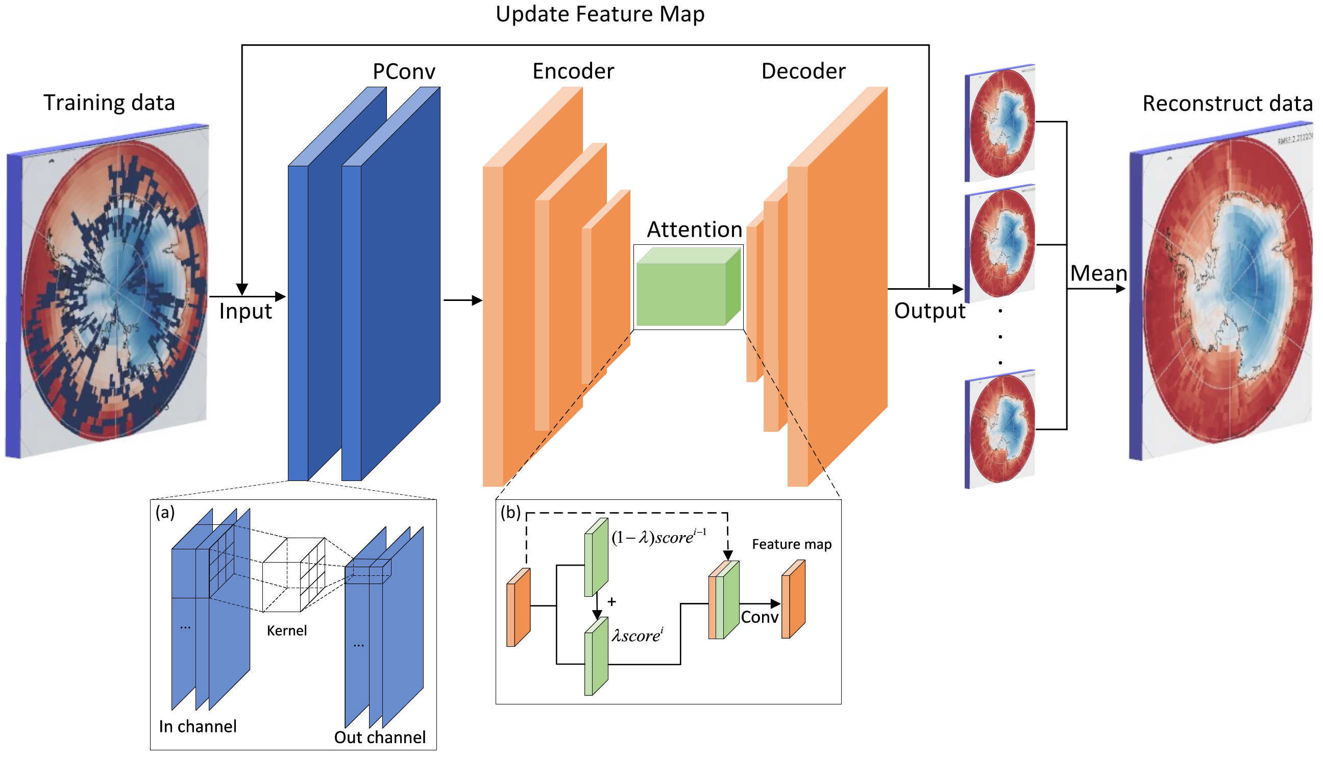
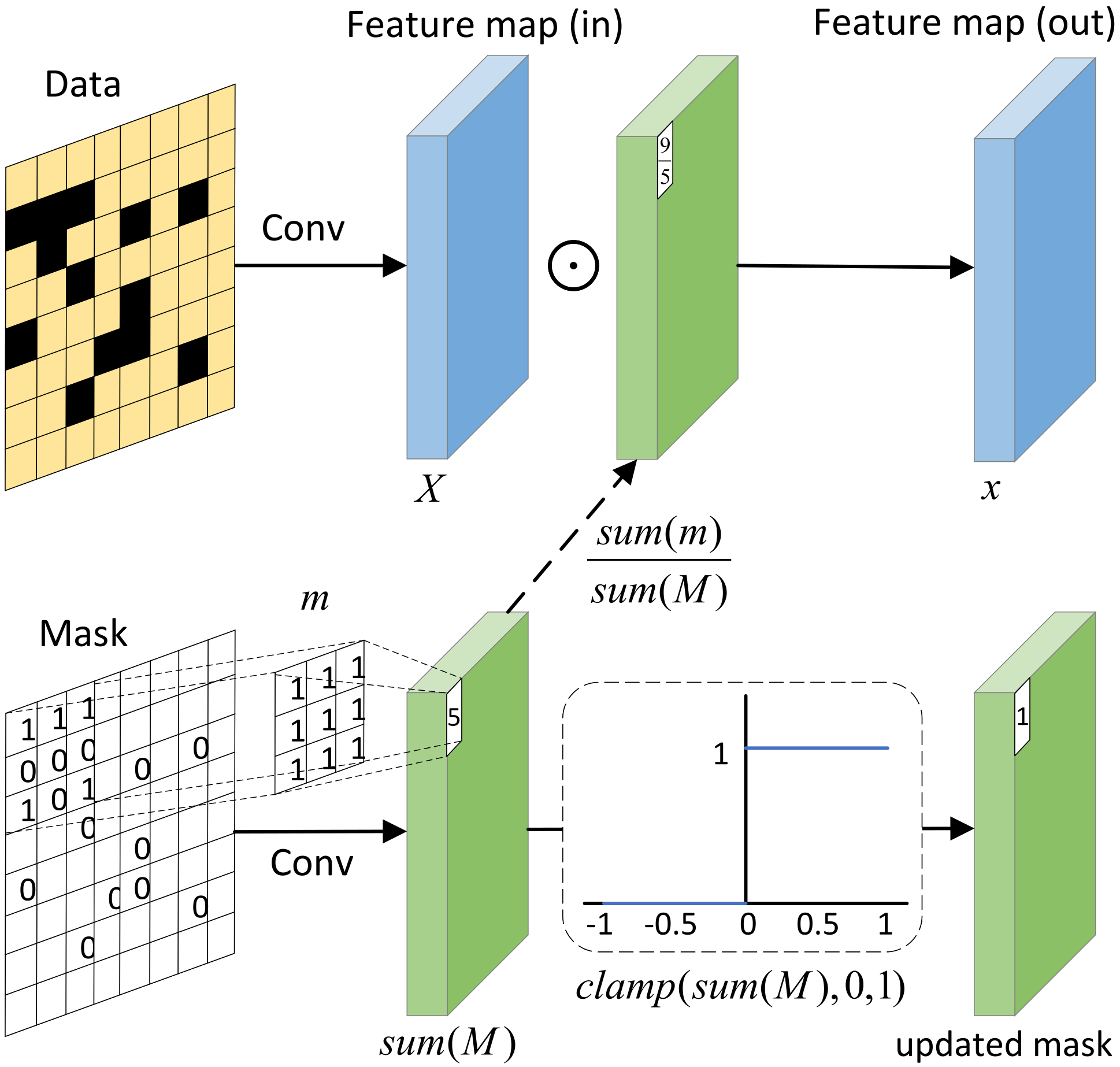
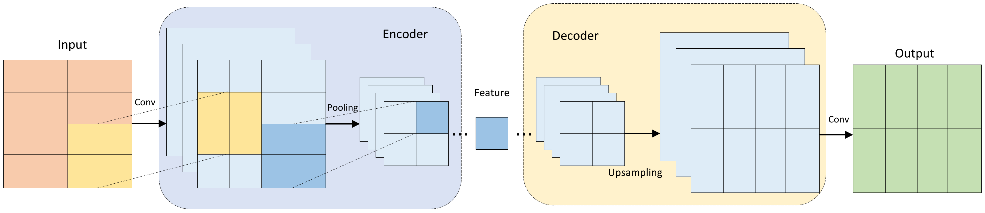
2. Methodology
2.1. Initialized by Spatial Pattern from Climate Model
2.2. Recurrent Feature Reasoning
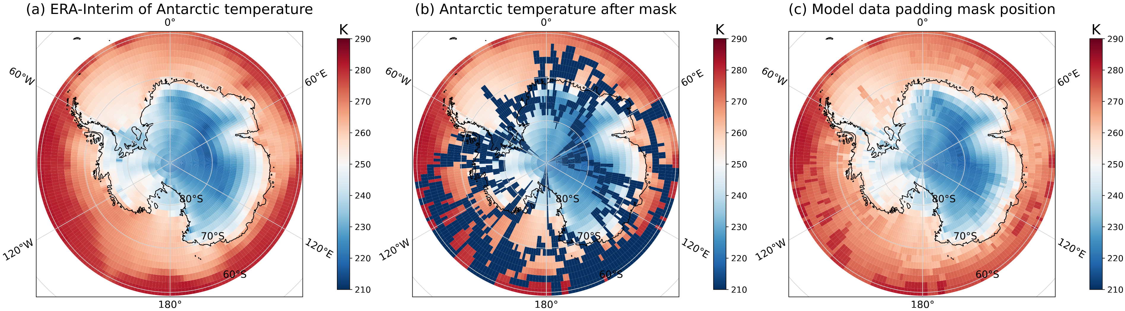
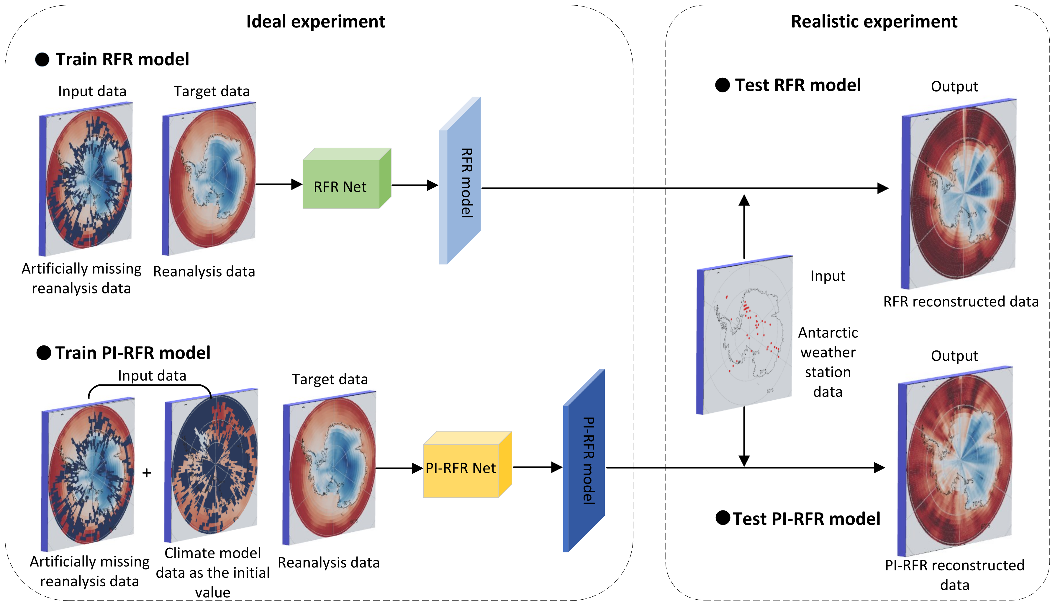
3. Data and Experiments
3.1. Ideal Experiments
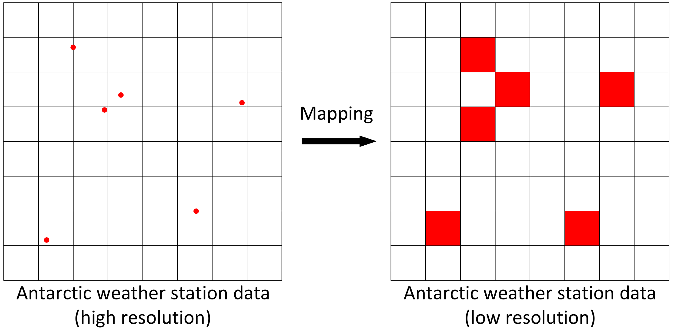
3.2. Realistic Experiments
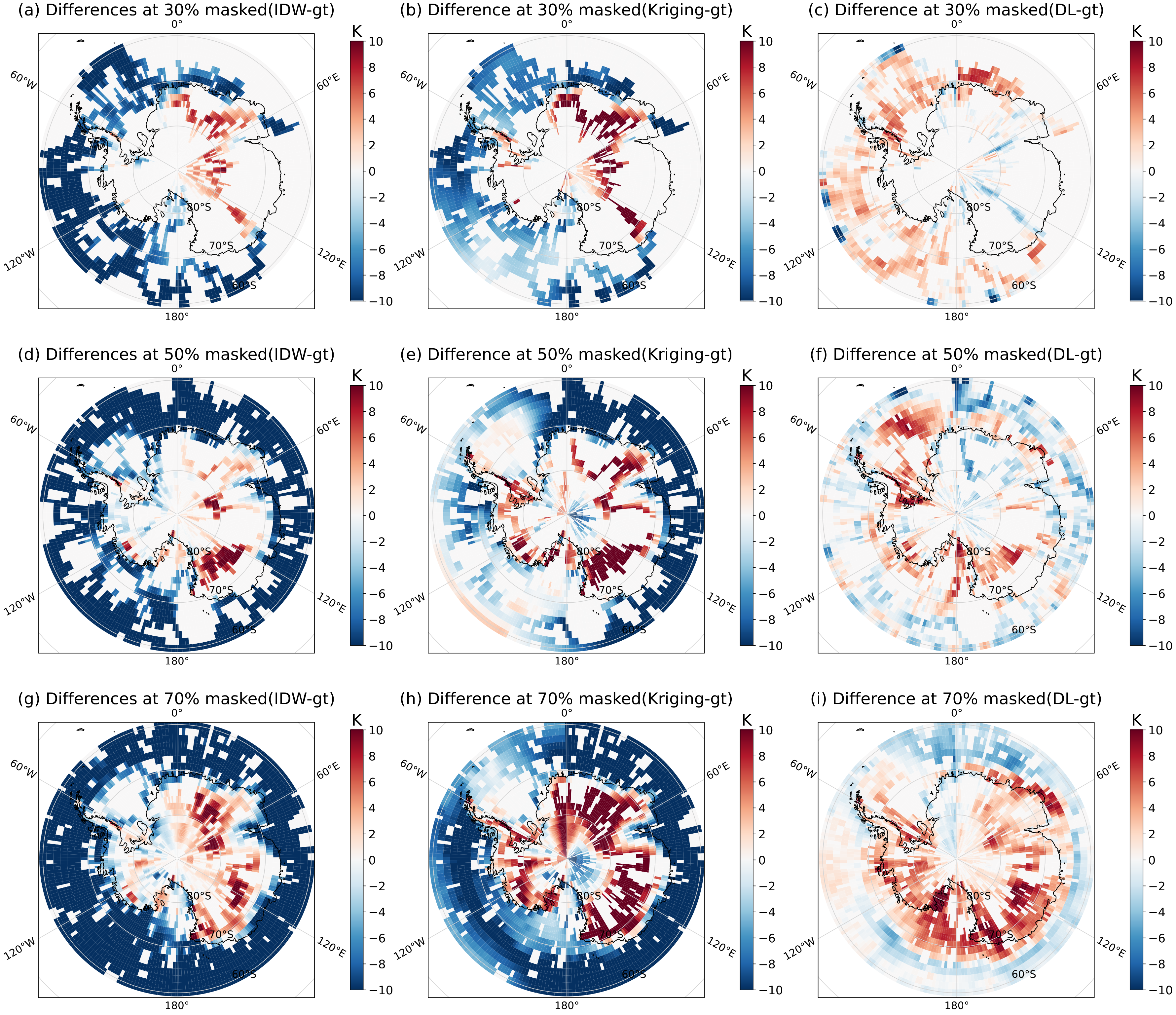
4. Results
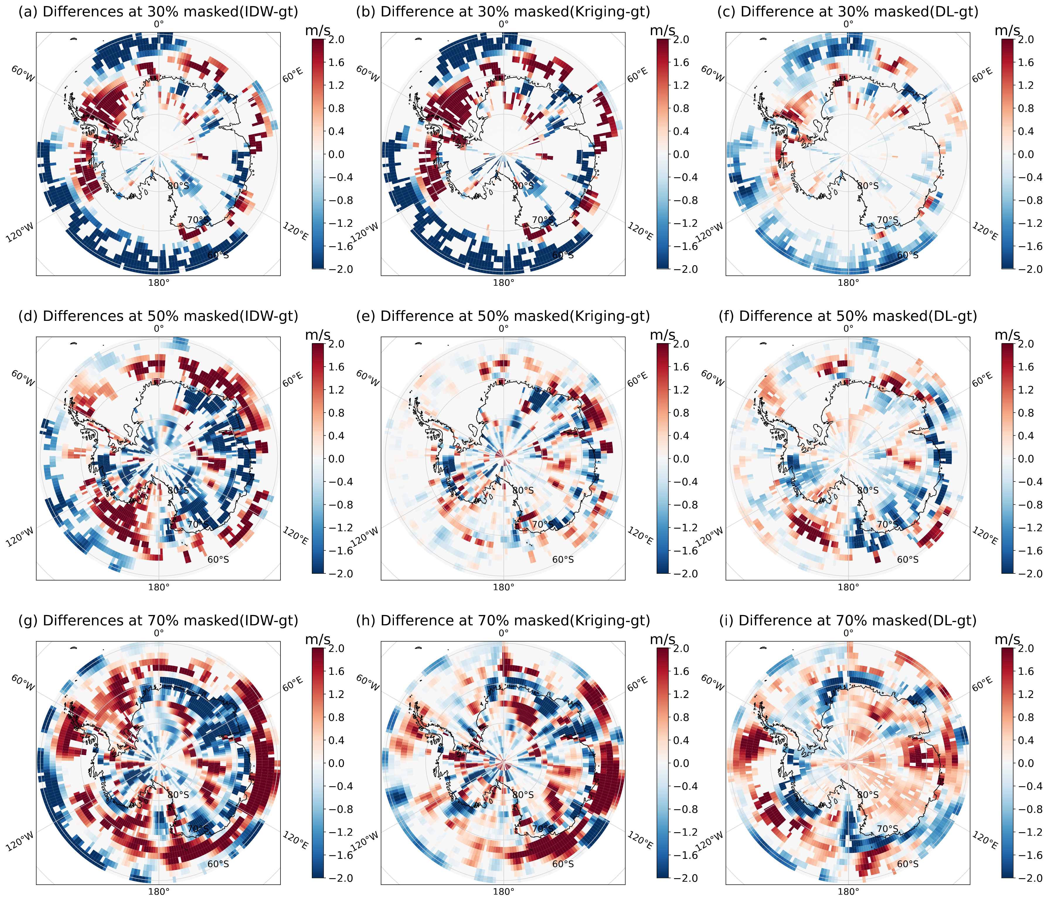
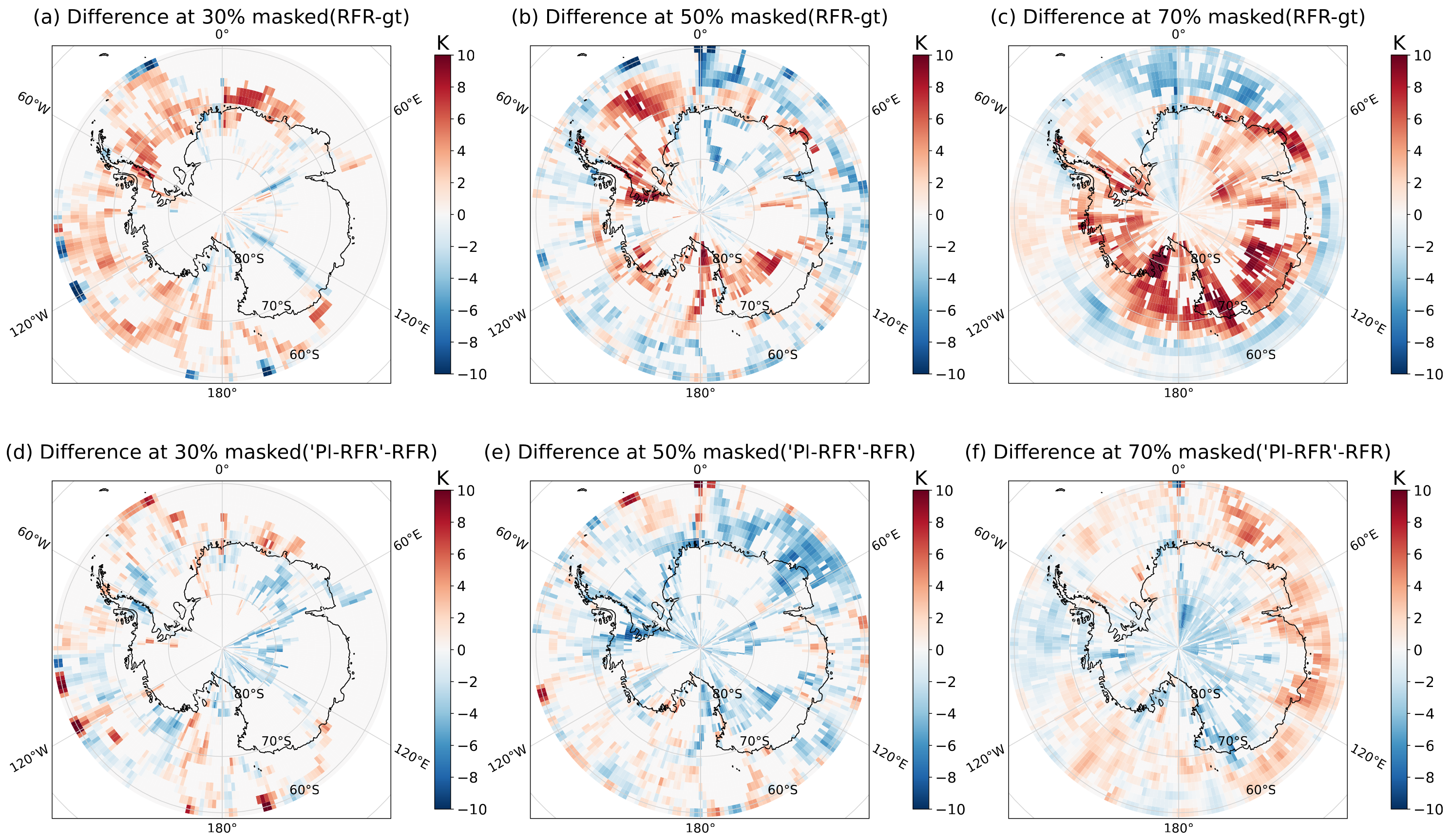
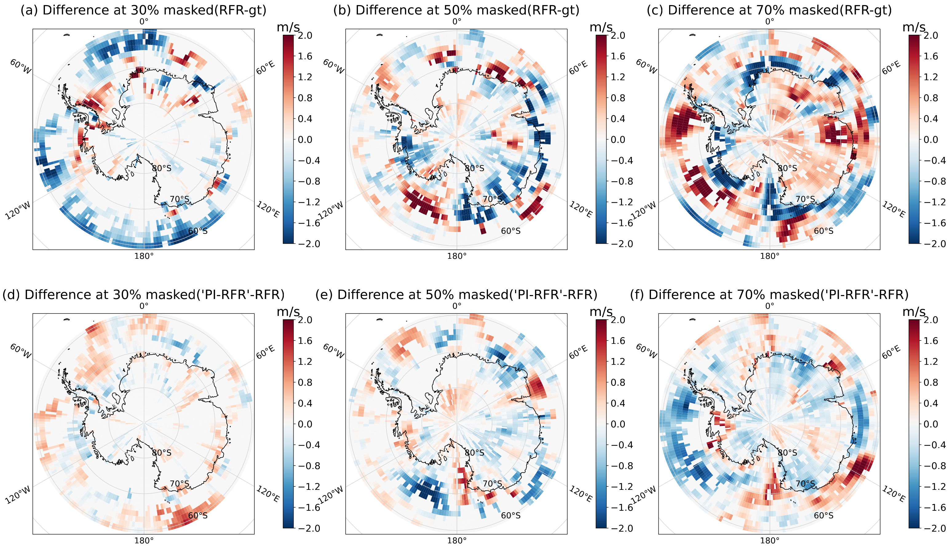
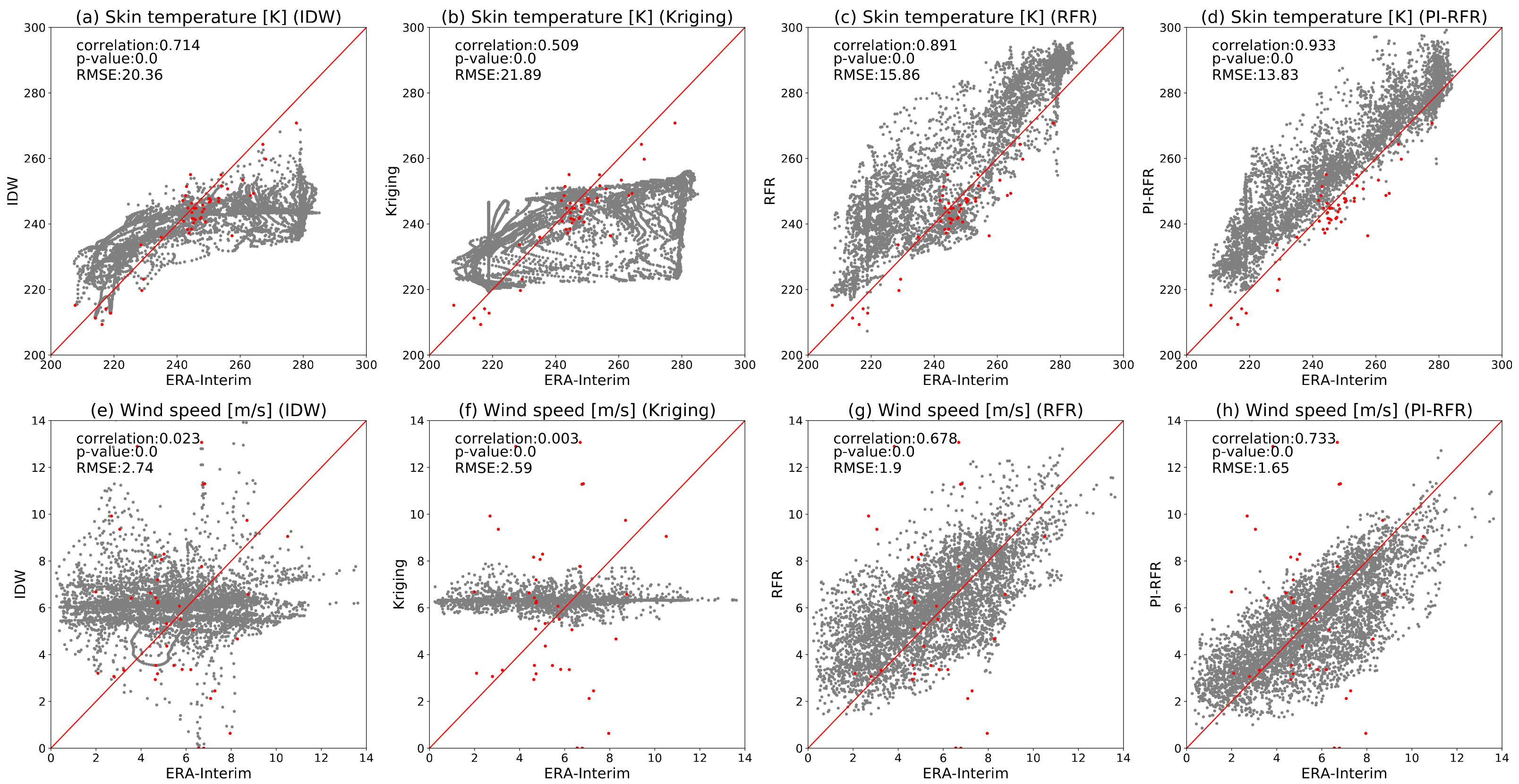
4.1. Comparison of the RFR with Traditional Methods
4.2. Comparison of the PI-RFR with RFR
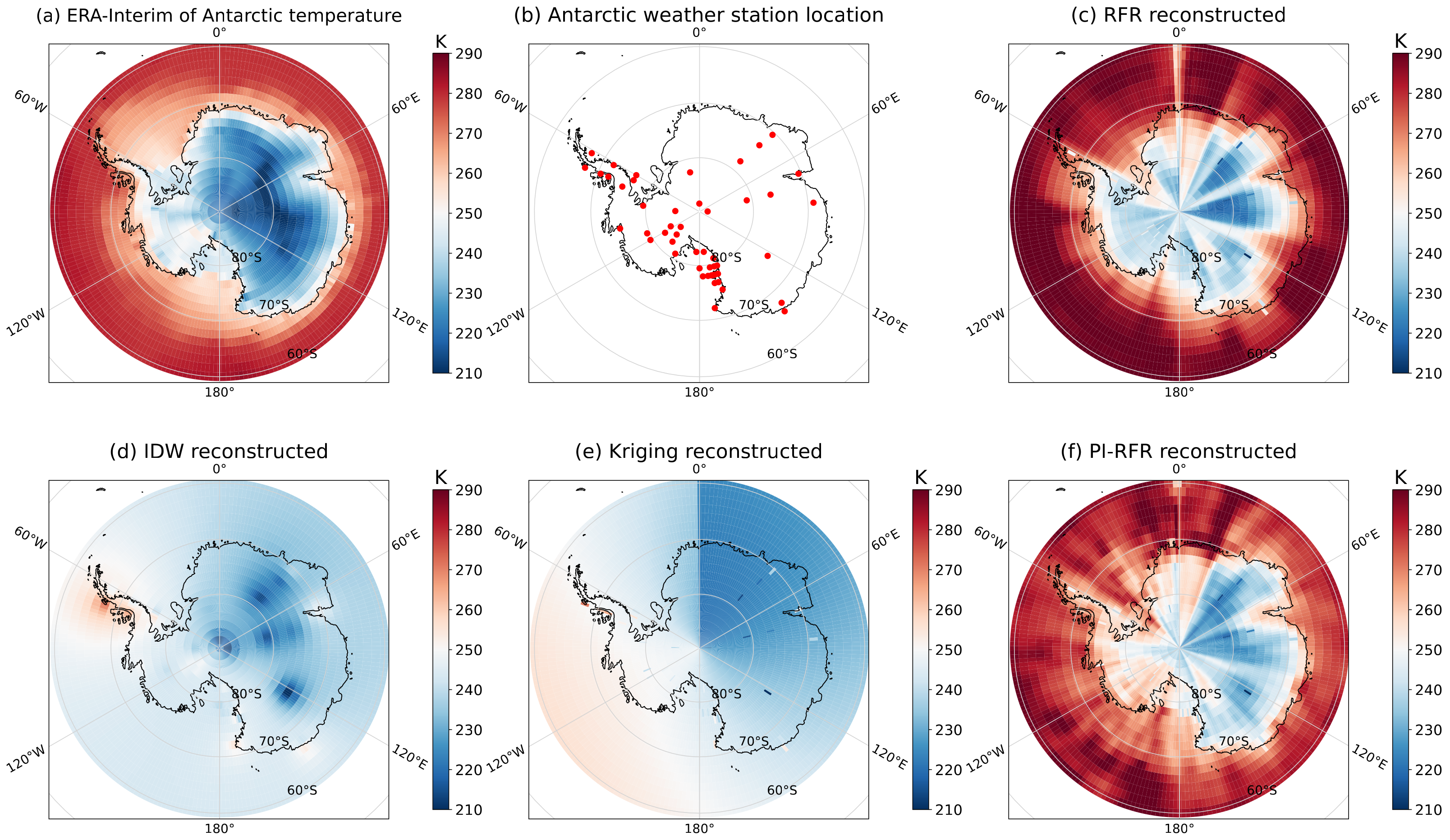
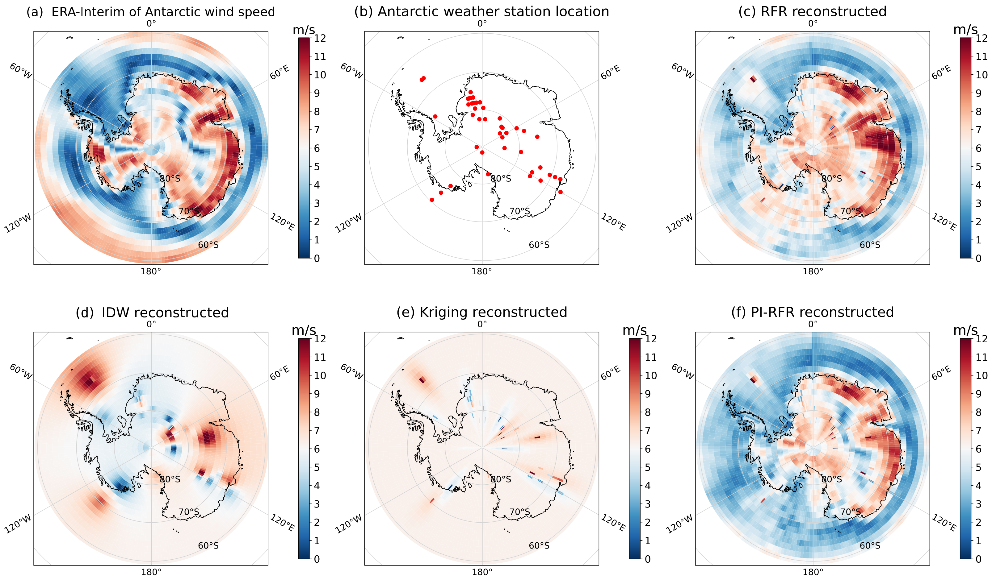
4.3. Reconstruction from Antarctic Site Data
5. Conclusions and Future Work
Author Contributions
Funding
Institutional Review Board Statement
Informed Consent Statement
Data Availability Statement
Acknowledgments
Conflicts of Interest
Abbreviations
| IDW | Inverse Distance Weighted |
| RFR | Recurrent Feature Reasoning |
| PI-RFR | Physics-Informed Recurrent Feature Reasoning |
| ECMWF | European Centre for Medium-Range Weather Forecasts |
| AI | Artificial Intelligence |
| GAN | Generative Adversarial Network |
| CNN | Convolutional Neural Network |
| SST | Sea Surface Temperature |
| E3SM | Energy Exascale Earth System Model |
| AMRC | Antarctic Meteorological Research Center |
| AWS | Automatic Weather Station |
| VGG | Visual Geometry Group |
| MDPI | Multidisciplinary Digital Publishing Institute |
References
- Rintoul, S.R.; Chown, S.L.; DeConto, R.M.; England, M.H.; Fricker, H.A.; Masson-Delmotte, V.; Naish, T.R.; Siegert, M.J.; Xavier, J.C. Choosing the future of Antarctica. Nature 2018, 558, 233–241. [Google Scholar] [CrossRef]
- Liu, J.; Bromwich, D.; Chen, D.; Cordero, R.; Jung, T.; Raphael, M.; Turner, J.; Yang, Q. Preface to the Special Issue on Antarctic Meteorology and Climate: Past, Present and Future. Adv. Atmos. Sci. 2020, 37, 421–422. [Google Scholar] [CrossRef]
- Parkinson, C.L. A 40-y record reveals gradual Antarctic sea ice increases followed by decreases at rates far exceeding the rates seen in the Arctic. Proc. Natl. Acad. Sci. USA 2019, 116, 14414–14423. [Google Scholar] [CrossRef] [PubMed] [Green Version]
- Edwards, T.L.; Nowicki, S.; Marzeion, B.; Hock, R.; Goelzer, H.; Seroussi, H.; Jourdain, N.C.; Slater, D.A.; Turner, F.E.; Smith, C.J.; et al. Projected land ice contributions to twenty-first-century sea level rise. Nature 2021, 593, 74–82. [Google Scholar] [CrossRef] [PubMed]
- Lazzara, M.A.; Weidner, G.A.; Keller, L.M.; Thom, J.E.; Cassano, J.J. Antarctic automatic weather station program: 30 years of polar observation. Bull. Am. Meteorol. Soc. 2012, 93, 1519–1537. [Google Scholar] [CrossRef]
- Hersbach, H.; Bell, B.; Berrisford, P.; Hirahara, S.; Horányi, A.; Muñoz-Sabater, J.; Nicolas, J.; Peubey, C.; Radu, R.; Schepers, D.; et al. The ERA5 global reanalysis. Q. J. R. Meteorol. Soc. 2020, 146, 1999–2049. [Google Scholar] [CrossRef]
- Rodwell, M.; Palmer, T. Using numerical weather prediction to assess climate models. Q. J. R. Meteorol. Soc. 2007, 133, 129–146. [Google Scholar] [CrossRef]
- Matheron, G. Principles of geostatistics. Econ. Geol. 1963, 58, 1246–1266. [Google Scholar] [CrossRef]
- Shepard, D. A Two-Dimensional Interpolation Function for Irregularly-Spaced Data; Association for Computing Machinery: New York, NY, USA, 1968. [Google Scholar]
- Hock, R.; Jensen, H. Application of kriging interpolation for glacier mass balance computations. Geogr. Ann. Ser. Phys. Geogr. 1999, 81, 611–619. [Google Scholar] [CrossRef]
- Mair, A.; Fares, A. Throughfall characteristics in three non-native Hawaiian forest stands. Agric. For. Meteorol. 2010, 150, 1453–1466. [Google Scholar] [CrossRef]
- Dhamodaran, S.; Lakshmi, M. Comparative analysis of spatial interpolation with climatic changes using inverse distance method. J. Ambient. Intell. Humaniz. Comput. 2021, 12, 6725–6734. [Google Scholar] [CrossRef]
- Bronowicka-Mielniczuk, U.; Mielniczuk, J.; Obroślak, R.; Przystupa, W. A comparison of some interpolation techniques for determining spatial distribution of nitrogen compounds in groundwater. Int. J. Environ. Res. 2019, 13, 679–687. [Google Scholar] [CrossRef] [Green Version]
- Kim, Y. Convolutional Neural Networks for Sentence Classification. arXiv 2014, arXiv:1408.5882. [Google Scholar]
- Zhang, T.; Lin, W.; Lin, Y.; Zhang, M.; Yu, H.; Cao, K.; Xue, W. Prediction of tropical cyclone genesis from mesoscale convective systems using machine learning. Weather. Forecast. 2019, 34, 1035–1049. [Google Scholar] [CrossRef]
- Zhang, T.; Lin, W.; Vogelmann, A.M.; Zhang, M.; Xie, S.; Qin, Y.; Golaz, J.C. Improving convection trigger functions in deep convective parameterization schemes using machine learning. J. Adv. Model. Earth Syst. 2021, 13, e2020MS002365. [Google Scholar] [CrossRef]
- Liu, G.; Reda, F.A.; Shih, K.J.; Wang, T.C.; Tao, A.; Catanzaro, B. Image inpainting for irregular holes using partial convolutions. In Proceedings of the European Conference on Computer Vision (ECCV), Munich, Germany, 8–14 September 2018; pp. 85–100. [Google Scholar]
- Goodfellow, I.; Pouget-Abadie, J.; Mirza, M.; Xu, B.; Warde-Farley, D.; Ozair, S.; Courville, A.; Bengio, Y. Generative adversarial nets. Adv. Neural Inf. Process. Syst. 2014, 27, 139–144. [Google Scholar]
- Krizhevsky, A.; Sutskever, I.; Hinton, G.E. Imagenet classification with deep convolutional neural networks. Adv. Neural Inf. Process. Syst. 2012, 25, 84–90. [Google Scholar] [CrossRef] [Green Version]
- Dong, J.; Yin, R.; Sun, X.; Li, Q.; Yang, Y.; Qin, X. Inpainting of remote sensing SST images with deep convolutional generative adversarial network. IEEE Geosci. Remote. Sens. Lett. 2018, 16, 173–177. [Google Scholar] [CrossRef]
- Shibata, S.; Iiyama, M.; Hashimoto, A.; Minoh, M. Restoration of sea surface temperature satellite images using a partially occluded training set. In Proceedings of the 2018 24th International Conference on Pattern Recognition (ICPR), Beijing, China, 20–24 August 2018; IEEE: Piscataway, NJ, USA, 2018; pp. 2771–2776. [Google Scholar]
- Leinonen, J.; Guillaume, A.; Yuan, T. Reconstruction of cloud vertical structure with a generative adversarial network. Geophys. Res. Lett. 2019, 46, 7035–7044. [Google Scholar] [CrossRef] [Green Version]
- Dewi, C.; Chen, R.C.; Liu, Y.T.; Yu, H. Various Generative Adversarial Networks Model for Synthetic Prohibitory Sign Image Generation. Appl. Sci. 2021, 11, 2913. [Google Scholar] [CrossRef]
- Li, J.; Wang, N.; Zhang, L.; Du, B.; Tao, D. Recurrent feature reasoning for image inpainting. In Proceedings of the IEEE/CVF Conference on Computer Vision and Pattern Recognition, Seattle, WA, USA, 13–19 June 2020; pp. 7760–7768. [Google Scholar]
- Yu, J.; Lin, Z.; Yang, J.; Shen, X.; Lu, X.; Huang, T.S. Generative image inpainting with contextual attention. In Proceedings of the PIEEE Conference on Computer Vision and Pattern Recognition, Salt Lake City, UT, USA, 18–23 June 2018; pp. 5505–5514. [Google Scholar]
- Kadow, C.; Hall, D.M.; Ulbrich, U. Artificial intelligence reconstructs missing climate information. Nat. Geosci. 2020, 13, 408–413. [Google Scholar] [CrossRef]
- Monteleoni, C.; Schmidt, G.A.; McQuade, S. Climate informatics: Accelerating discovering in climate science with machine learning. Comput. Sci. Eng. 2013, 15, 32–40. [Google Scholar] [CrossRef] [Green Version]
- Badrinarayanan, V.; Kendall, A.; Cipolla, R. Segnet: A deep convolutional encoder-decoder architecture for image segmentation. IEEE Trans. Pattern Anal. Mach. Intell. 2017, 39, 2481–2495. [Google Scholar] [CrossRef] [PubMed]
- Simmons, A.; Willett, K.; Jones, P.; Thorne, P.; Dee, D. Low-frequency variations in surface atmospheric humidity, temperature, and precipitation: Inferences from reanalyses and monthly gridded observational data sets. J. Geophys. Res. Atmos. 2010, 115, D01110. [Google Scholar] [CrossRef] [Green Version]
- Uppala, S.; Dee, D.; Kobayashi, S.; Berrisford, P.; Simmons, A. Towards a climate data assimilation system: Status update of ERA-Interim. ECMWF Newsl. 2008, 115, 12–18. [Google Scholar]
- Dee, D.P.; Uppala, S.M.; Simmons, A.J.; Berrisford, P.; Poli, P.; Kobayashi, S.; Andrae, U.; Balmaseda, M.; Balsamo, G.; Bauer, d.P.; et al. The ERA-Interim reanalysis: Configuration and performance of the data assimilation system. Q. J. R. Meteorol. Soc. 2011, 137, 553–597. [Google Scholar] [CrossRef]
- Golaz, J.C.; Van Roekel, L.P.; Zheng, X.; Roberts, A.F.; Wolfe, J.D.; Lin, W.; Bradley, A.M.; Tang, Q.; Maltrud, M.E.; Forsyth, R.M.; et al. The DOE E3SM Model Version 2: Overview of the physical model and initial model evaluation. J. Adv. Model. Earth Syst. 2022, 14, e2022MS003156. [Google Scholar] [CrossRef]


| Skin Temperature | Wind Speed | |||||
|---|---|---|---|---|---|---|
| Missing Rate | IDW | Kriging | RFR | IDW | Kriging | RFR |
| 30% | 5.08 | 3.96 | 1.72 | 1.06 | 0.83 | 0.48 |
| 50% | 8.94 | 6.77 | 2.46 | 1.25 | 0.84 | 0.62 |
| 70% | 12.01 | 9.48 | 3.07 | 1.46 | 1.28 | 0.79 |
| Skin Temperature | Wind Speed | |||
|---|---|---|---|---|
| Missing Rate | RFR | PI-RFR | RFR | PI-RFR |
| 30% | 1.72 | 1.68 | 0.48 | 0.42 |
| 50% | 2.46 | 1.89 | 0.62 | 0.59 |
| 70% | 3.07 | 2.94 | 0.79 | 0.71 |
Disclaimer/Publisher’s Note: The statements, opinions and data contained in all publications are solely those of the individual author(s) and contributor(s) and not of MDPI and/or the editor(s). MDPI and/or the editor(s) disclaim responsibility for any injury to people or property resulting from any ideas, methods, instructions or products referred to in the content. |
© 2023 by the authors. Licensee MDPI, Basel, Switzerland. This article is an open access article distributed under the terms and conditions of the Creative Commons Attribution (CC BY) license (https://creativecommons.org/licenses/by/4.0/).
Share and Cite
Yao, Z.; Zhang, T.; Wu, L.; Wang, X.; Huang, J. Physics-Informed Deep Learning for Reconstruction of Spatial Missing Climate Information in the Antarctic. Atmosphere 2023, 14, 658. https://doi.org/10.3390/atmos14040658
Yao Z, Zhang T, Wu L, Wang X, Huang J. Physics-Informed Deep Learning for Reconstruction of Spatial Missing Climate Information in the Antarctic. Atmosphere. 2023; 14(4):658. https://doi.org/10.3390/atmos14040658
Chicago/Turabian StyleYao, Ziqiang, Tao Zhang, Li Wu, Xiaoying Wang, and Jianqiang Huang. 2023. "Physics-Informed Deep Learning for Reconstruction of Spatial Missing Climate Information in the Antarctic" Atmosphere 14, no. 4: 658. https://doi.org/10.3390/atmos14040658