

Decomposing Fast and Slow Responses of Global Cloud Cover to Quadrupled CO2 Forcing in CMIP6 Models
1
State Key Laboratory of Severe Weather, Chinese Academy of Meteorological Sciences, Beijing 100081, China
2
University of Chinese Academy of Sciences, Beijing 100049, China
3
Collaborative Innovation Center on Forecast and Evaluation of Meteorological Disasters, Nanjing University of Information Science and Technology, Nanjing 210044, China
4
Laboratory for Climate Studies of China Meteorological Administration, National Climate Center, Beijing 100081, China
*
Author to whom correspondence should be addressed.
Atmosphere 2023, 14(4), 653; https://doi.org/10.3390/atmos14040653
Submission received: 8 March 2023
/
Revised: 27 March 2023
/
Accepted: 28 March 2023
/
Published: 30 March 2023
(This article belongs to the Special Issue Climate Change and Climate Variability, and Their Impact on Extreme Events)
Abstract
:Cloud changes and their attribution under global warming still remains a challenge in climatic change studies, especially in decomposing the fast and slow cloud responses to anthropogenic forcing. In this study, the responses of global cloud cover to the quadrupled CO2 forcing are investigated quantitatively by decomposing the total response into fast and slow ones using the multi-model data from the Coupled Model Intercomparison Project Phase 6 (CMIP6). During the quasi-equilibrium period after the quadrupling of CO2 forcing, the global mean changes of simulated total cloud cover (TCC) in the total, fast, and slow responses are −2.42%, −0.64%, and −1.78%, respectively. Overall, the slow response dominates the total response in most regions over the globe with similar spatial patterns. TCC decreases at middle and low latitudes but increases at high latitudes in the total and slow responses. Whereas, it mainly decreases in the middle and low latitudes of the southern hemisphere as well as in the middle and high latitudes of the northern hemisphere in the fast response. A change in vertical motion is the major contributor to the cloud cover change at middle and low latitudes, while the decrease in upper atmospheric temperature leads to an increase in high cloud cover at high latitudes. In addition, the anomaly in water vapor convergence/diffusion also contributes to the cloud cover increase/decrease at low latitudes.
1. Introduction
Clouds cover about two thirds of the Earth’s surface and play an important role in the Earth’s radiative energy balance [1,2,3]. The effect of clouds on the radiation balance consists of two main processes [4]: on the one hand, clouds can reflect large amounts of shortwave radiation, which reduces the surface downward shortwave radiation and leads to a cooling effect; on the other hand, clouds absorb a large part of longwave radiation emitted from the surface, which reduces the energy loss to outer space and causes a warming effect. Changes in cloud cover can affect the climate system through altering their radiative effects. Randall et al. [5] demonstrated that a 4% increase in low clouds can offset the warming effect caused by the doubled CO2, otherwise the warming effect is expected to be amplified. As the largest uncertainty source in the climate change research [6,7,8,9,10], studies on clouds would hopefully improve our understanding of future climate change.
Many researchers have reported the observed changes in cloud cover in the past decades [11,12,13,14,15,16,17]. Ding et al. [11] pointed out that the global mean total cloud cover (TCC) showed a decreasing trend, with a substantial decrease in the tropics and mid-latitudes and an increase in high latitudes. Norris et al. [16] demonstrated that greenhouse gases emitted into the atmosphere by human activities are the most significant external forcing factor affecting the cloud changes in recent decades. As an important tool for evaluating future climate change, global climate models (GCMs) have played an important role in studying the impact of the increasing CO2 on cloud cover, but demonstrate opposite results in different studies. For example, some early studies found that an increase in CO2 concentration could lead to an increase in low cloud cover in the tropics [18,19], whereas an opposite trend was found in some recent studies [20,21]. Wetherald [22] demonstrate that the climate sensitivities in models could affect the simulations of cloud cover; in particular, low clouds in the tropics and subtropics increase (decrease) in models with lower (higher) surface warming caused by a doubled CO2. All these studies above suggest a considerable uncertainty in the responses of simulated clouds to increasing the CO2 concentration.
The climate responses to a forcing factor can be decomposed into the fast and the slow responses [10,23,24,25]. The fast responses represent the adjustments of circulation, clouds, water vapor, and precipitation due to forcing-induced atmospheric radiative heating before the global surface air temperature (SAT) changes, while the slow responses are changes in a range of physical quantities owing to forcing-induced changes in global SAT. The timescale of the fast response ranges from days to months, while it can be extended from years to decades for the slow response. Hansen et al. [26] proposed a method called ‘fixed-SST’ to obtain the fast response in a climate model, i.e., using climatologic sea surface temperature (SST) and sea ice (SI) in the model regardless of ocean changes. The slow response is the difference between the total response and the fast response [27,28,29,30].
The fast response of clouds, also called rapid adjustment or fast feedback, may reduce the Earth energy imbalance caused by the doubled CO2 [31]. The fast cloud response is generally represented by a decrease in cloud cover in climate models [32,33,34,35]. Dinh and Fueglistaler [36] demonstrated that the fast cloud responses caused by an increasing CO2 concentration include an increase and decrease in cloud cover in the boundary layer and the free troposphere, respectively. However, Wyant et al. [37] demonstrated slight increases in total, low, and high cloud cover but with a slight decrease in medium cloud cover over the globe and tropics under the quadrupled CO2 forcing in a superparameterized climate model, and Xu et al. [38] also supported this result.
The studies on decomposition of the fast and slow cloud responses demonstrated that changes in cloud cover caused by increasing CO2 are mainly manifested as an increase in high cloud cover and a decrease in middle and low cloud cover in both fast and slow responses [39,40,41]. A doubled CO2 experiment demonstrated that the total cloud cover decreased over land and ocean in the fast response, while in the slow response, the high cloud cover increased and the mid-low cloud cover decreased over the ocean [39]. Andrew and Ringer [40] used the HadGEM2-ES model to investigate the fast and slow cloud responses, and they found an increase in high cloud cover and a decrease in mid-low cloud cover all over the globe, land, and ocean; moreover, the slow response dominate the cloud changes at all altitudes globally and over the ocean. Zelinka et al. [41] used the ISCCP (International Satellite Cloud Climatology Project) simulator in CMIP5 to distinguish the responses of different types of clouds according to the cloud top height and cloud optical depth; their results demonstrated that the global mean low and middle cloud cover decreased and high cloud cover increased in both fast and slow responses, and the clouds changed from thin to thick and from a low level to high level in the slow response with global warming.
Up to now, only a few studies work on the decomposition of the total cloud responses into the fast and slow ones to understand deeply the mechanism of cloud change under the background of global warming. Zhou et al. [42] used a GCM named BCC–AGCM2.0 to investigate the fast and slow responses caused by quadrupled CO2 concentration over East Asia, and found that the total response is dominated by the slow response, and the cloud changes are determined by the variations in atmospheric circulation, temperature, and water vapor. The fast and slow cloud responses on global scales, however, need to be further investigated in the future work. This study aims to investigate the fast and slow responses of global clouds to the quadrupled CO2 to understand the mechanism between them. Since the cloud responses to the increasing CO2 vary greatly among different models, the multi-model mean outputs from CMIP6 are used in this study to reduce the differences between models. The purpose of this study is to explore the cloud responses on different temporal scales and to point out which response dominates the cloud changes under the quadrupled CO2 warming.
2. Materials and Methods
2.1. CMIP6 Model Experiments
The Coupled Model Intercomparison Project (CMIP), sponsored by the World Climate Research Programme (WCRP), aims to better understand the past, present, and future climate change caused by natural variability or anthropogenic forcing [43]. In this study, the multi-model outputs from the CMIP Phase 6 (CMIP6) are used to investigate the cloud cover responses to the quadrupled CO2 forcing. Four sets of CMIP6 experiments are described as below.
- 1)
- piControl: The pre-industrial control simulation is one of the CMIP6 DECK (Diagnosis Evaluation and Characterization of Klima) experiments, which is driven in a fully coupled Atmosphere-Ocean general circulation model (AOGCM) under conditions chosen to be representative of the period prior to the onset of large-scale industrialization, with 1850 being the reference year. All forcings are kept at 1850 levels, which include CO2 and other well-mixed greenhouse gases (WMGHG), aerosols, and precursors, ozone, stratospheric water vapour, land use, volcanoes, solar irradiance, and the cosmic ray. The piControl starts after an initial climate spin-up, during which the climate begins to come into balance with the forcing, then runs for at least 500 years. It can be used to study the unforced internal variability of the climate system due to the unchanged anthropogenic and natural forcings.
- 2)
- abrupt-4×CO2: The abrupt-4×CO2 simulation branches from some point in piControl, the CO2 concentration is immediately and abruptly quadrupled from the global annual mean 1850 value in an AOGCM, then runs for at least 150 years. All other anthropogenic and natural forcings are kept in 1850 levels, as with piControl. It can be used to estimate the climate system response to the quadrupled CO2.
- 3)
- piClim-control: The piClim-control simulation is driven by the pre-industrial control climatological SST and SI in an atmosphere-land model and runs for 30 years. The pre-industrial monthly averaged climatology of SST and SI was generated from at least a 30-year segment of the piControl experiment integration. All anthropogenic and natural forcings are kept in 1850 levels, as with piControl. This provides a baseline to calculate the effective radiative forcing and the fast climate response.
- 4)
- piClim-4×CO2: The piClim-4×CO2 simulation is driven by the pre-industrial control climatological SST and SI in an atmosphere-land model and runs for 30 years. The pre-industrial monthly averaged climatology of SST and SI was generated from at least a 30-year segment of the piControl experiment integration. The CO2 concentration is immediately and abruptly quadrupled from the global annual mean 1850 value, and all other anthropogenic and natural forcings are kept in 1850 levels, as with piControl and piClim-4×CO2. It can be used to estimate the fast climate response caused by the quadrupled CO2.
Table S1 lists a total of 44 modes that can be used to calculate the total response and 12 modes that can be used to calculate the fast response. In order to obtain usable slow responses, we selected outputs from 10 models because they are the only ones available in all four experiments, as shown in Table 1. In addition, the results using the 10 models and using all available models listed in Table S1 are largely robust (Figure S1).
2.2. Methodology to Calculate the Total, Fast, and Slow Responses
The total response caused by the quadrupled CO2 forcing can be deduced by the difference between the experiments abrupt-4×CO2 and piControl. The model outputs of these two experiments averaged from year 121 to 150 (i.e., the years of model arriving at quasi-equilibrium after the interruption) are therefore utilized to calculate the total response of TCC. According to the method provided by Hansen et al. [26], the fast response of TCC in this study can be calculated by the difference of experiments piClim-4×CO2 and piClim-control averaged over 30 years to obtain the climatology. The slow response can then be derived by subtracting the fast response from the total response [27,28,29,30]. Moreover, all model outputs in this study are interpolated to a horizontal resolution of 2.5° × 2.5°.
3. Results
3.1. Responses of TCC to the Quadrupled CO2 Forcing
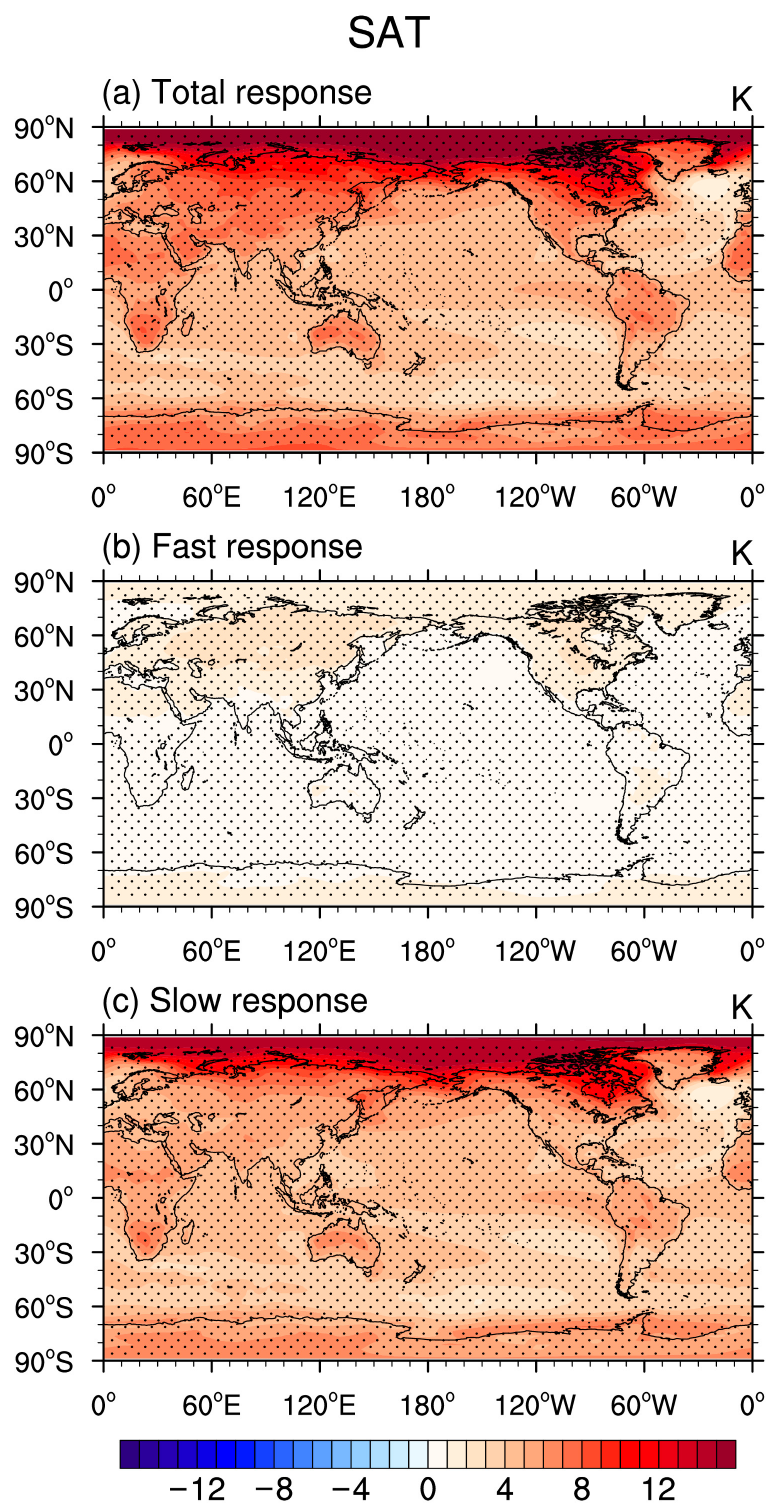
Figure 1 shows the total, fast, and slow responses of multi-model mean SAT over the globe to the quadrupled CO2 forcing. In both the total and slow responses, the ocean warms much more slowly than the land due to its higher heat capacity than that of the land. Most of the ocean warms by less than 4 K, while the land warming is generally above 5 K. The land warming in the northern hemisphere increases with increasing latitudes, with Arctic warming reaching to more than 15 K due to the Arctic amplification [44]. In the fast response, the SST is fixed and unchanged, while the largest land warming is located in northern Asia and some individual regions over North America. The global mean SAT changes are 5.31 K, 0.52 K, and 4.79 K in the total, fast, and slow responses, respectively, indicating that the global warming is mainly caused by the slow response. An increase in SAT will enhance surface evaporation, increase saturated water vapor pressure, and alter atmospheric circulation, leading to changes in cloud cover. Thus, our focus is mainly on the responses of global TCC in the following section.
Figure 2 presents the total, fast, and slow responses of the multi-model mean TCC over the globe to the quadrupled CO2 forcing. In the total response, the TCC decreases in most areas at low and middle latitudes, especially in southern Africa, the Mediterranean, Southeast Asia, the Japan Sea, the mid-latitude Pacific in the northern hemisphere, the Pacific near 30° S, Mexico, and Brazil. However, the TCC increases in high latitudes of the southern hemisphere, the Arctic Ocean, the tropical South Atlantic, and the tropical South Pacific, with significant increases of more than 10% in the equatorial Pacific and the subsidence region of the Walker circulation. In the fast response, the TCC decreases in northern Eurasia, North America, South America, the Atlantic, eastern South Pacific, the Indian Ocean, and the mid-latitudes of the southern hemisphere. The significant TCC increases appear in the central African continent and regions from the Arabian Peninsula to northern India, with other increase regions including the North Pacific, the western tropical South Pacific, the equatorial East Pacific, the Antarctic continent, and regions near the North Pole. The spatial distribution pattern of TCC changes in the slow response is similar to that in the total response, but with a larger reduction in central Africa and a smaller reduction in the Mediterranean. Compared to the total response, the TCC increase in the Arctic extends southward to the northern Eurasia and North America in the slow response, but the model numbers with the same sign are less than eight (80%) over these regions.
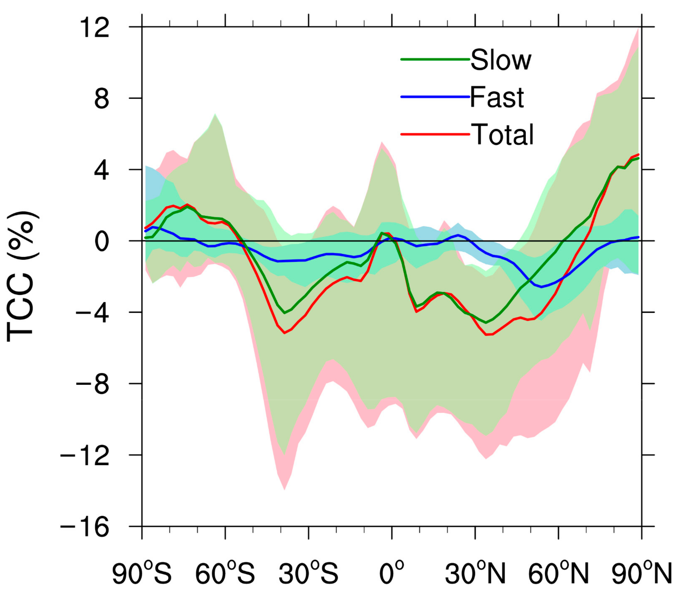
Figure 3 shows the zonal mean distributions of the global TCC responses. In the total and the slow responses, the TCC increases south of 55° S with their maximum values both reaching 2.0% at 75° S, while it decreases at 55° S–5° S and 0°–60° N with minimum values appearing at 40° S (about −5.5% and −4.0% in the total and slow responses) and 35° N (about −5.5% and −4.5% in the total and slow responses), respectively. The reason for the slight TCC increase near the equator is due to the significant TCC increase over the equatorial Pacific (Figure 2a,c). The TCC increases rapidly north of 70° N (60° N) in the total (slow) response, and reaches a maximum value (larger than 4.5%) near the North Pole. The magnitude of zonal mean change of TCC in the fast response is smaller than those in the total and slow responses. In the fast response, the TCC increases south of 70° S and decreases significantly at 70° S–0° and north of 30° N, with a minimum value around −2.5% at 55° N, while negligible TCC changes are noticed at 0°–30° N. Overall, in the total and slow responses, TCC decreases at middle and low latitudes and increases at high latitudes; in the fast response, TCC decreases at mid-low latitudes in the southern hemisphere and mid-high latitudes in the northern hemisphere, while it changes slightly at high latitudes in the southern hemisphere and low latitudes in the northern hemisphere.
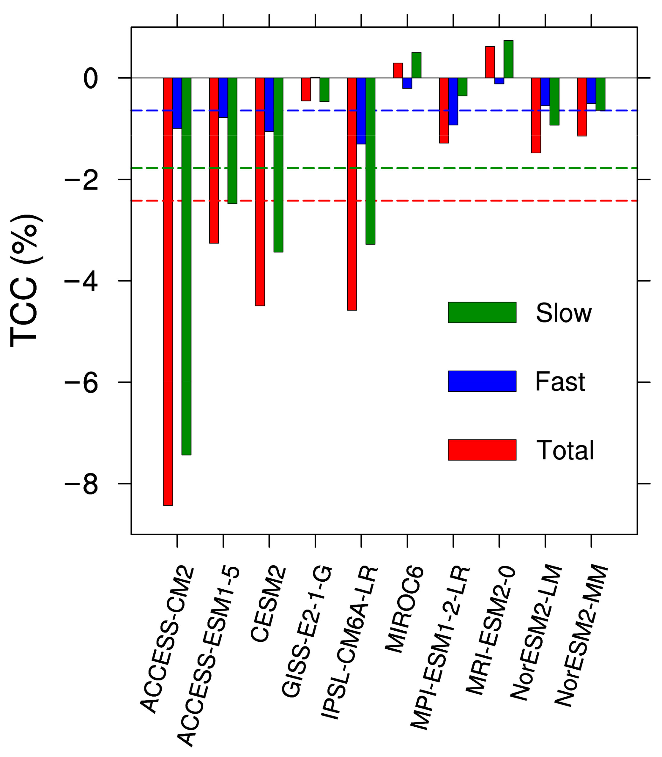
The global mean changes in TCC in the total, fast, and slow responses are −2.42%, −0.64%, and −1.78%, respectively (Table 2), which indicates that under the quadrupled CO2 forcing, the global TCC decreases in all three responses. The reduction in the slow response is larger than that in the fast response, accounting for 74.55% of the total response, suggesting that the slow TCC response dominates the total response of the global TCC. However, as shown in Figure 4, the TCC responses vary largely among models. For example, the total and slow responses of TCC in ACCESS-CM2 are as high as −8.43% and −7.43%, respectively, whereas they increase slightly in MIROC6 and MRI-ESM2.0. The uncertainty of the multi-model means of TCC change in the total response ranges from −8.43% to 0.62% with a median of −1.38%, while it varies in a range of −1.30% and 0.015% (−7.43% and 0.74%) with a median of −0.66% (−0.79%) in the fast (slow) response.
In this study, we only use outputs from the 10 models available in all four experiments. As a comparison, Figure S1 presents the total response of the global TCC from 44 available models and the fast response from 12 available models, respectively. The model information is listed in Table S1. The spatial distributions of the total and fast responses shown in Figure S1 are similar to Figure 1, which indicates that the simulations from 10 typical models used in this study are reliable.
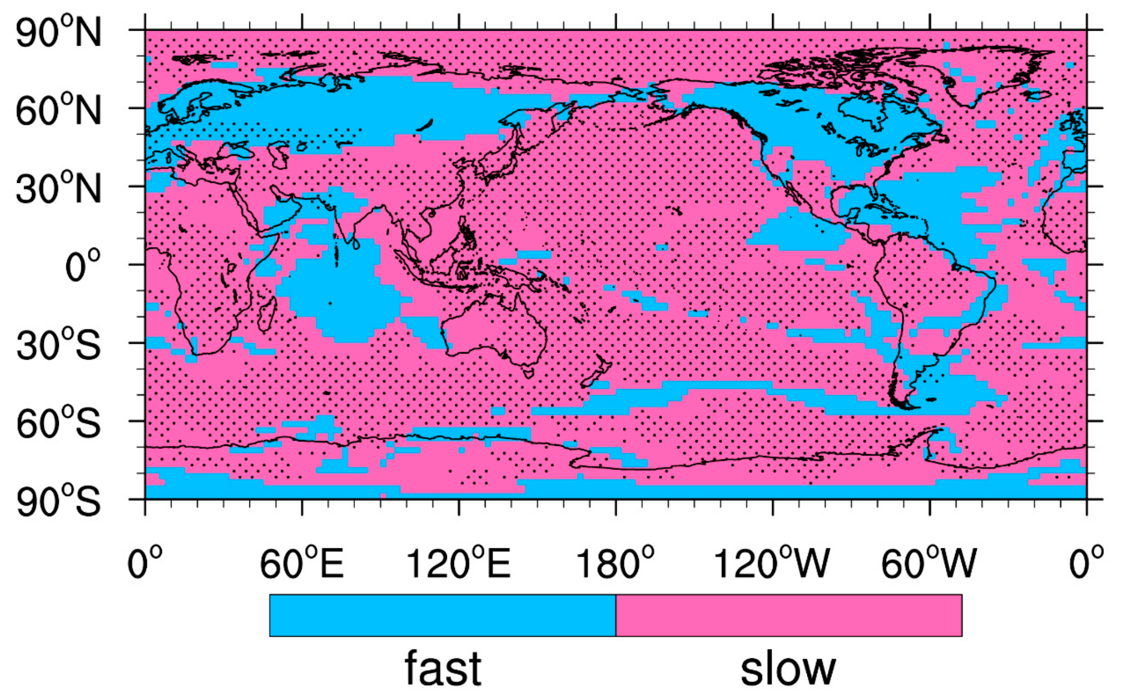
Figure 5 presents the dominated responses of global TCC changes. The regions in blue and pink colours indicate that they are dominated by the fast response and slow response, respectively. In general, the slow responses dominate the TCC changes in most regions, while regions dominated by the fast responses include northern Eurasia, the tropical Indian Ocean, most regions of North America, the western tropical North Atlantic, the western ocean beside Mexico, and the eastern ocean beside Argentina. However, less than eight (80%) models agree with the dominance of the fast response, suggesting worse agreement than the slow responses. Therefore, the model simulations of clouds in these regions need to be improved. More models should be encouraged to participate in the Coupled Model Intercomparison Project to improve the simulation of the fast response in the future.
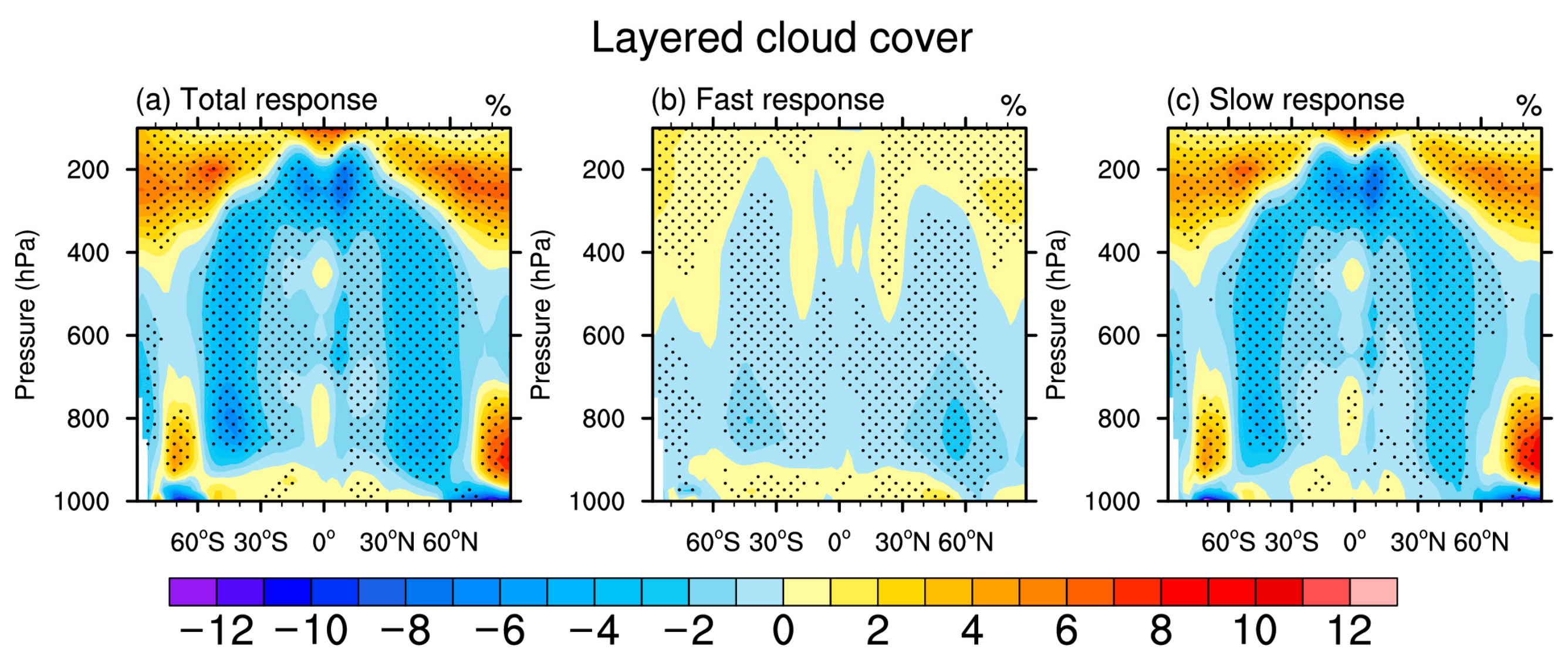
Figure 6 shows the distributions of global zonal mean changes of the layered cloud cover. In the total response, cloud cover at high latitudes of both hemispheres increases significantly in the upper atmosphere at pressures less than 400 hPa, while it decreases in the middle atmosphere at 400–700 hPa. At 70° N–90° N and 60° S–80° S latitudes, cloud cover increases significantly in the lower atmosphere at pressures greater than 700 hPa. Therefore, the increases in TCC in the Arctic and high latitudes of the southern hemisphere in Figure 2a are contributed to by both high and low clouds. At the mid-latitudes in both hemispheres, cloud cover increases in the upper atmosphere, but decreases at most pressure levels. The TCC in the total response thus decreases at mid-latitudes in both hemispheres (Figure 2a). At low latitudes, cloud cover decreases significantly in the upper atmosphere at 150–300 hPa on both sides of the equator, while it mainly decreases in the middle and lower atmosphere at pressures greater than 300 hPa with a small change near the equator. This is possibly because that the significant increase in cloud cover in the equatorial Pacific Ocean and the subsidence region of the Walker circulation is largely offset by the cloud cover decrease in other regions at low latitudes (Figure 2a). In addition, an increase in cloud cover occurs near the surface at middle and low latitudes. In the fast response, cloud cover at high latitudes of both hemispheres increases in the middle and upper atmosphere at pressures less than 600 hPa, but decreases in the middle and lower atmosphere at pressures greater than 600 hPa. The largest increase in cloud cover is found in the upper atmosphere near the two poles, causing an increase in TCC (Figure 2b). The cloud cover decreases mainly at middle and low latitudes, but increases near the surface. The most significant decrease is found in the atmosphere between 700 hPa and 900 hPa at the mid-latitudes, leading to the TCC decrease at the mid-latitudes (Figure 2b). The distribution of the slow response of the layered cloud cover is similar to the total response. However, the increase in the low (high) cloud cover in the slow response at high latitudes of the northern hemisphere is larger (smaller) than that in the total response. Moreover, the decreases in cloud cover at mid-latitudes of both hemispheres in the slow response are smaller than that in the total response, which is consistent with Figure 3. Our results indicate that the global TCC and layered cloud cover are both dominated by the slow response, which is consistent with those over East Asia that are documented by Zhou et al. [42].
It should be noted that the TCC in a global climate model is contributed by not only a layer cloud cover but also a convective cloud cover. Figure S2 shows the distribution of a convective cloud cover from the piControl experiment in nine available CMIP6 models (Table S2) as well as the difference between experiments abrupt-4xCO2 and piControl. In the tropics, the strong convection leads to the formation of high convective clouds, with large variations in the equatorial Pacific and Atlantic. However, only a few models in CMIP6 provide outputs of a convective cloud cover; thus, it is necessary to add more information on the convective cloud cover in future model comparison projects to improve the understanding of cloud responses in climate change.
3.2. Mechanisms of TCC Changes in the Total, Fast, and Slow Responses
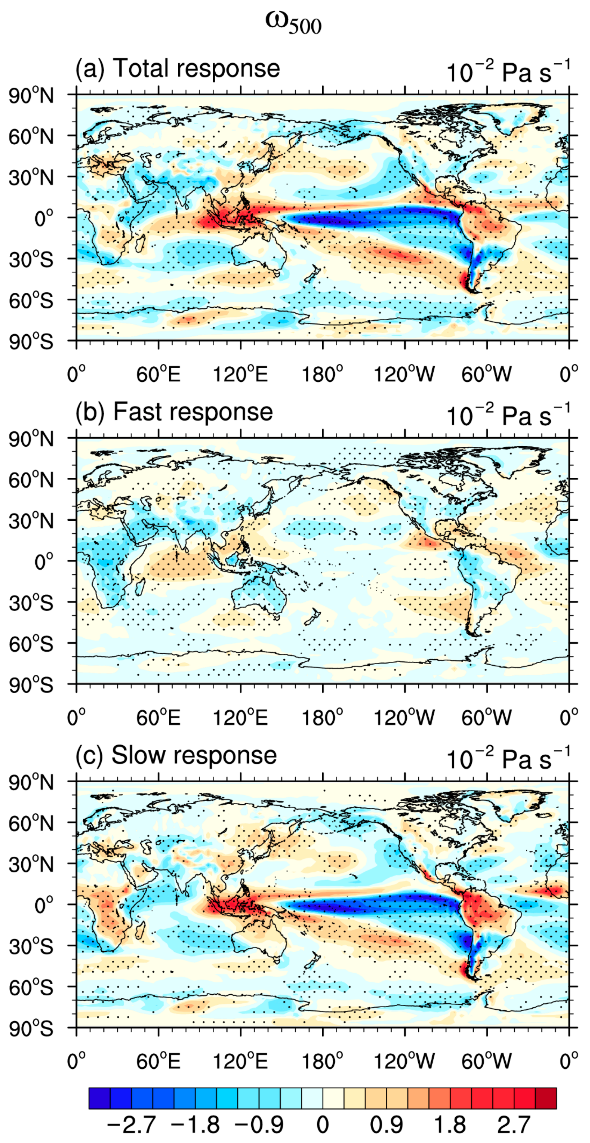
The vertical velocity at 500 hPa (ω500) can reflect the strength of the convection, and the strong convective ascending motion is beneficial to the formation of clouds. Figure 7 presents the distributions of the changes in 500 hPa vertical velocity, where positive and negative values represent descending and ascending motion anomalies, respectively. The pronounced changes in ω500 at low latitudes are closely related to the strong convective motions over these regions. The opposite changes in ω500 at middle and low latitudes have a high consistency with the changes in TCC (Figure 2), especially at low latitudes. In the total and slow responses, the strong positive anomalies of ω500 in Southeast Asia and Brazil significantly contribute to the TCC reduction, while the remarked TCC increase in the equatorial Pacific Ocean and the subsidence region of Walker circulation is highly associated with the strong negative anomalies of ω500. Moreover, the positive anomalies of ω500 also appear in central Africa, the Mediterranean, southern China, the mid-latitude North Pacific and South Atlantic, and the South Pacific around 30° S, resulting in a decrease in the TCC there. However, the negative anomaly of ω500 over the ocean near 60° S is conductive to the increase in TCC. In the fast response, the notable positive anomalies of ω500 occurs in the low-latitude Indian Ocean, South China Sea, Central Asia, oceans beside Mexico, Atlantic, and eastern South Pacific, and the notable negative anomalies occur in the African continent, Arabian Peninsula, India, Chinese continent, Australia, and low-latitude North Pacific, respectively, contributing to the reduction and increase in TCC over these regions.
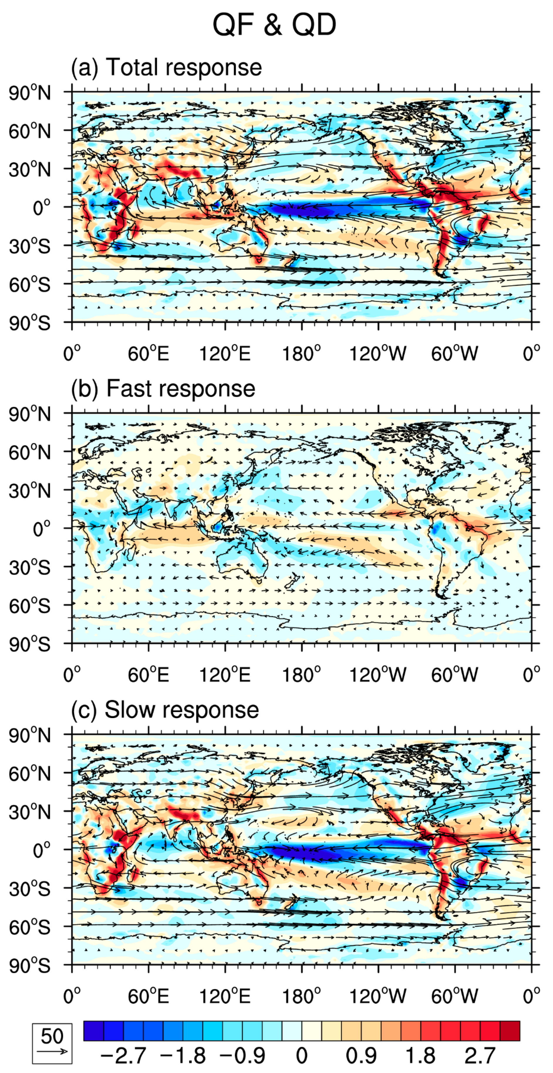
Water vapor supply plays an important role in cloud formation and maintenance [45]. Figure 8 shows the changes in the vertical integrated column water vapor flux (referred to as QF) and divergence (referred to as QD) in the whole atmosphere, where positive and negative values represent anomalous water vapor diffusion and convergence, respectively. The water vapor flux divergence varies greatly due to the abundance of water vapor in the tropics, and the reverse changes in QD at low latitudes are highly related to the changes in TCC (Figure 2). In both the total and slow responses, anomalous water vapor diffusions in the coast of Africa, the Arabian Peninsula, the Tibet Plateau, the low-latitude Indian Ocean in the southern hemisphere, Southeast Asia, Japan Sea, Central America, Brazil, Chile, and South Pacific around 30° S contribute to the reduction in TCC, while the strong anomalous water vapor convergence in the equatorial Pacific results in a large increase in TCC. In the fast response, the anomalous water vapor diffusions in the low-latitudes of the Indian Ocean and Atlantic Ocean, Central America, and majority of Eurasia lead to the reduction in TCC, while the increase in TCC in central Africa, the Arabian Peninsula, the western North Pacific, as well as Australia and its eastern ocean results from the anomalous water vapor convergences over these regions.
The changes in vertical integrated column water vapor fluxes and divergences in the lower, middle, and upper atmosphere are also shown in Figures S3–S5. Generally, in the total and slow responses, the different distributions of QD changes in the lower, middle, and upper atmosphere are in agreement with the TCC changes at different altitudes. In the lower atmosphere, the anomalous water vapor diffusions in the coast of Africa, the low-latitude Indian Ocean in the southern Hemisphere, and Central America result in a decrease in cloud cover, while the anomalous water vapor convergence in the equatorial Pacific leads to an increase in cloud cover. In the middle atmosphere, anomalous water vapor diffusions in inland Africa, Brazil, and Chile give rise to the decreasing cloud cover. The increase in TCC in the eastern South Pacific at low latitudes is caused by the anomalous water vapor convergences in the middle and upper atmosphere. Due to the high altitude of the Tibet Plateau, the decrease in TCC in the Tibet Plateau mainly results from the anomalous water vapor diffusion in the upper atmosphere. In the fast response, since the water vapor changes in the middle and upper atmosphere are small and not significant, the changes in cloud cover are therefore mainly determined by the QD changes in the lower atmosphere.
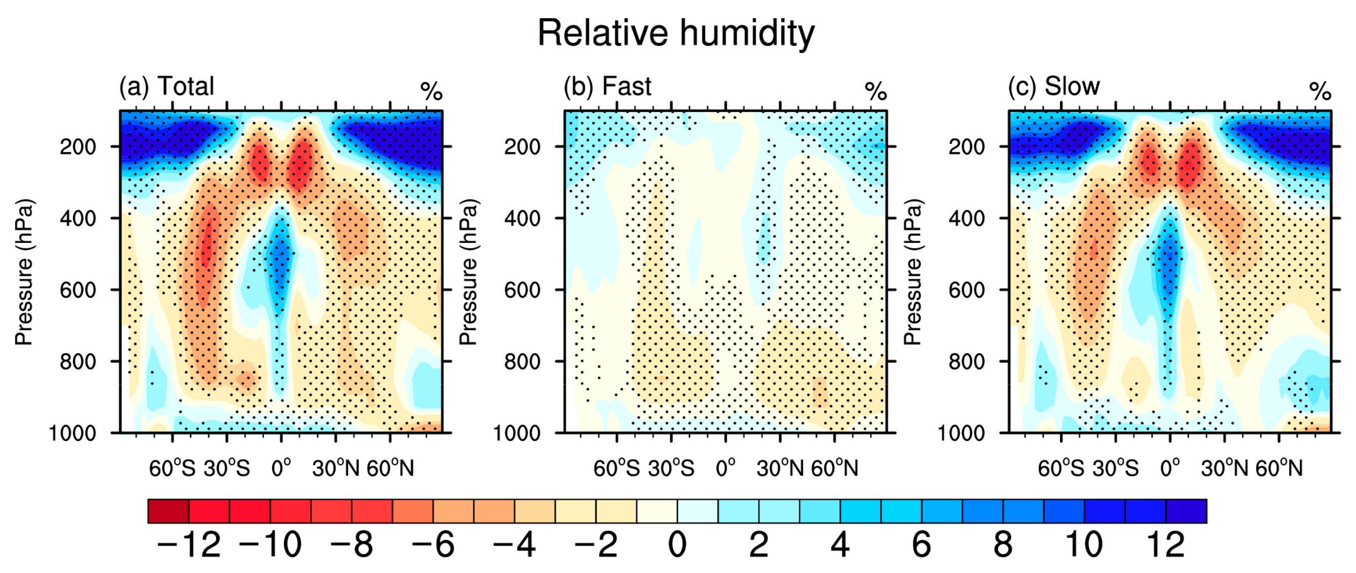
Relative humidity (RH) is an important determinant of cloud cover. Figure 9 presents the distributions of the global zonal mean changes in the RH with air pressure, which is in good agreement with the distributions of a layered cloud cover (Figure 6). In the total and the slow responses, the increases in the RH at high latitudes in the upper and lower atmosphere cause an increase in cloud cover, while the largest decrease in the RH at mid-latitudes also corresponds to the largest reduction in cloud cover (Figure 3). However, the significant decreases in the RH at low latitudes in the upper atmosphere at 150–300 hPa on both sides of the equator cause a remarked decrease in cloud cover. In the middle atmosphere, the RH around the equator increases significantly, which is mainly caused by the large increase in the RH over the Pacific Ocean around the equator (Figure S6), resulting in an increase in medium clouds in this region. In the fast response, the increase in the RH at high latitudes in the upper atmosphere lead to an increase in high clouds, and the decreases in both the RH and cloud cover in the lower atmosphere at 700–900 hPa are the largest at mid-latitudes. In addition, in all the total, fast, and slow responses, an increase in the RH occurs near the surface at middle and low latitudes, leading to an increase in cloud cover near the surface.
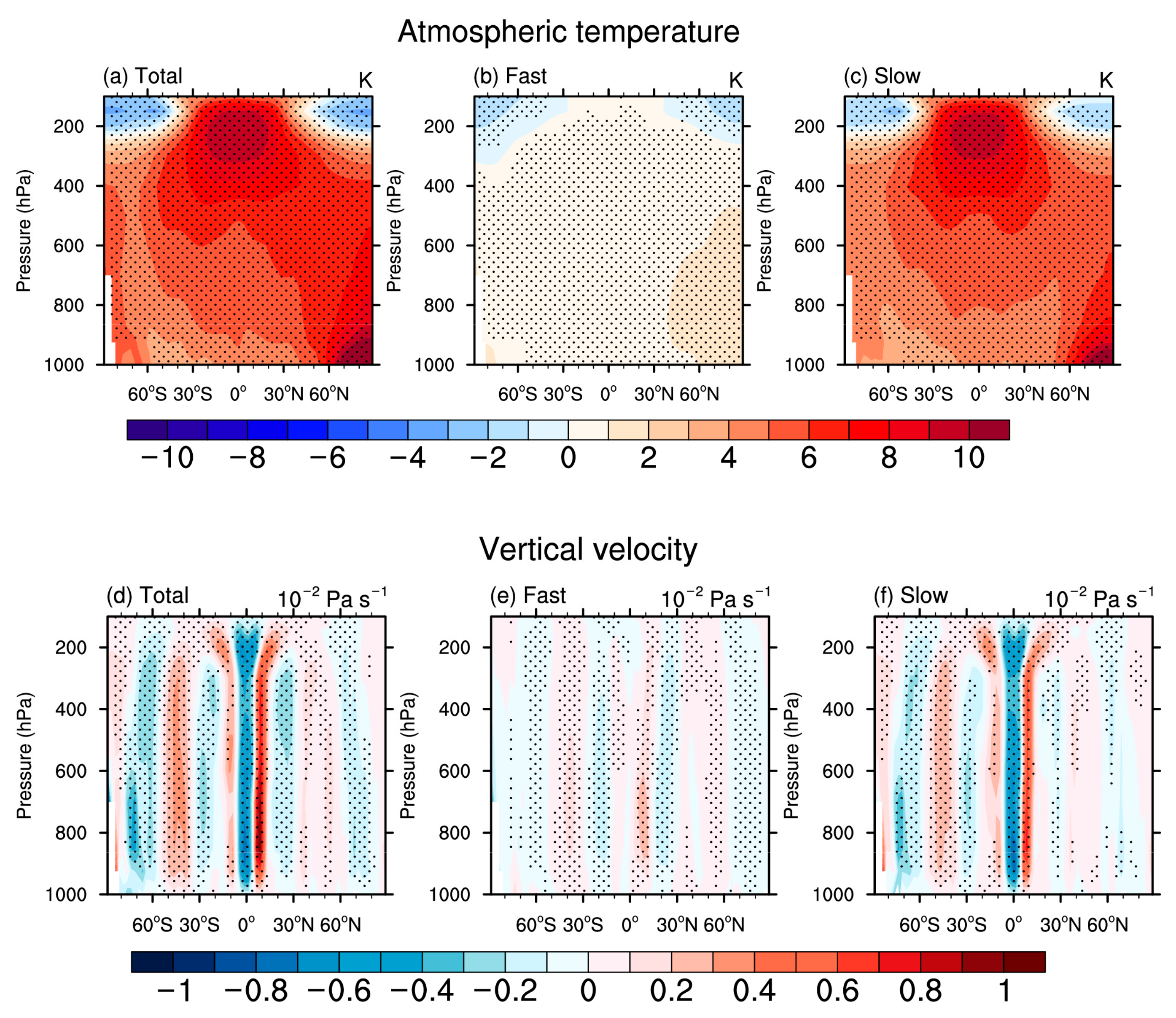
The increase in atmospheric temperature can increase the saturated water vapor pressure, playing an important role in reducing the RH and cloud cover, while the enhancement in the atmospheric vertical ascending motion contributes to the increase in cloud cover. Thus, our focus in the following study is to analyse the effects of the atmospheric temperature and vertical velocity changes on the RH and cloud cover. Figure 10a–c gives the distributions of global zonal mean changes in the atmospheric temperature with air pressure. At high latitudes, the temperature in the upper atmosphere decreases in all the three responses, which reduces the saturated water vapor pressure, resulting in a significant increase in the RH and high cloud cover in the upper atmosphere. In the total and slow responses, the upper atmospheric temperature increases dramatically at low latitudes, which causes an increase in the saturated water vapor pressure, leading to a significant decrease in the upper atmospheric RH and high cloud cover. At middle and low latitudes, the surface warmings in all three responses are smaller than the atmospheric warmings above the surface, which enhance the intensity of the boundary layer inversion and atmospheric static stability. This makes it difficult for the water vapor near the surface to break through the boundary layer, thus accumulating near the surface and resulting in an increase in the near-surface RH and cloud cover.
Figure 10d–f shows the distributions of the global zonal mean vertical velocity changes with air pressure, where positive and negative values represent anomalous descending and ascending motions, respectively. In the total and slow responses, strong ascending motion anomalies occur on the equator, which is mainly due to the strong ascending motion anomalies in the equatorial Pacific, as shown in Figure 7, resulting in an increase in the RH and cloud cover in the lower and middle atmosphere over this region. However, anomalous descending motions on both sides of the equator lead to a decrease in cloud cover. In the upper atmosphere at low latitudes, the increase in atmospheric temperature leads to an increase in the saturated water vapor pressure, which greatly reduces the RH and high cloud cover. However, the anomalous ascending motion on the equator transports water vapor to the upper atmosphere, which partly offsets the decrease in the RH and high cloud cover in the upper equatorial atmosphere. In both hemispheres, the anomalous descending motions at mid-latitudes cause a significant decrease in the low and medium cloud cover, while the anomalous ascending motions at high latitudes contribute to an increase in the low cloud cover. In the fast response, the general anomalous descending motions at middle and low latitudes reduce the low and medium cloud cover over most regions. However, Figure 10e shows an anomalous ascending motion near 20° S and 20° N, which results from the anomalous ascending motion over Africa, the Arabian Peninsula, India, Australia, and the North Pacific at these latitudes (Figure 7b), resulting in an increase in TCC (Figure 2b), and mainly a high cloud cover (Figure 6b).
Compared to the fast response, more significant changes appear in the atmospheric temperature, vertical motion, and water vapor in the slow response due to the participation of the ocean, resulting in more substantial changes in cloud cover. Particularly, the dramatic ascending air motion anomaly and abundant water vapor supply in the slow response in the equatorial Pacific are the major contributors to the large increase in the TCC.
3.3. Analysis of Cloud Responses in Typical Regions
According to Figure 2, the magnitude of TCC changes in tropics is large with decreasing trends at middle latitudes. We select three typical regions in the tropics and one typical region at the mid-latitude North Pacific for the detailed analysis. Their geographic ranges are given as follows: A: 15° S–15° N, 15–35° E; B: 10° S–10° N, 100° E–130° E; C: 0–20° S, 130° W–100° W; D: 30° N–50° N, 170° E–160° W.
Region A is located in central Africa, where TCC decreases significantly in both the total and slow responses (−5.12% and −8.13%, respectively), but with a remarked increase in the fast response (3.01%). As the ascending region of the Walker circulation, Region B is located in Southeast Asia with TCC decreases in the total, fast, and slow responses (−6.76%, −0.82%, and −5.94%, respectively). Region C is located in the eastern tropical South Pacific, which is the subsidence region of the Walker circulation, where TCC increases significantly in both the total and slow responses (9.95% and 11.09%, respectively) but decreases in the fast response (−1.14%). Region D is located in the mid-latitude North Pacific, where TCC decreases prominently in the total and slow responses (−5.95% and −6.39%, respectively) but increases slightly in the fast response (0.44%). The fast and slow responses of TCC are opposite in regions A, C, and D, but it is another case for the region B.
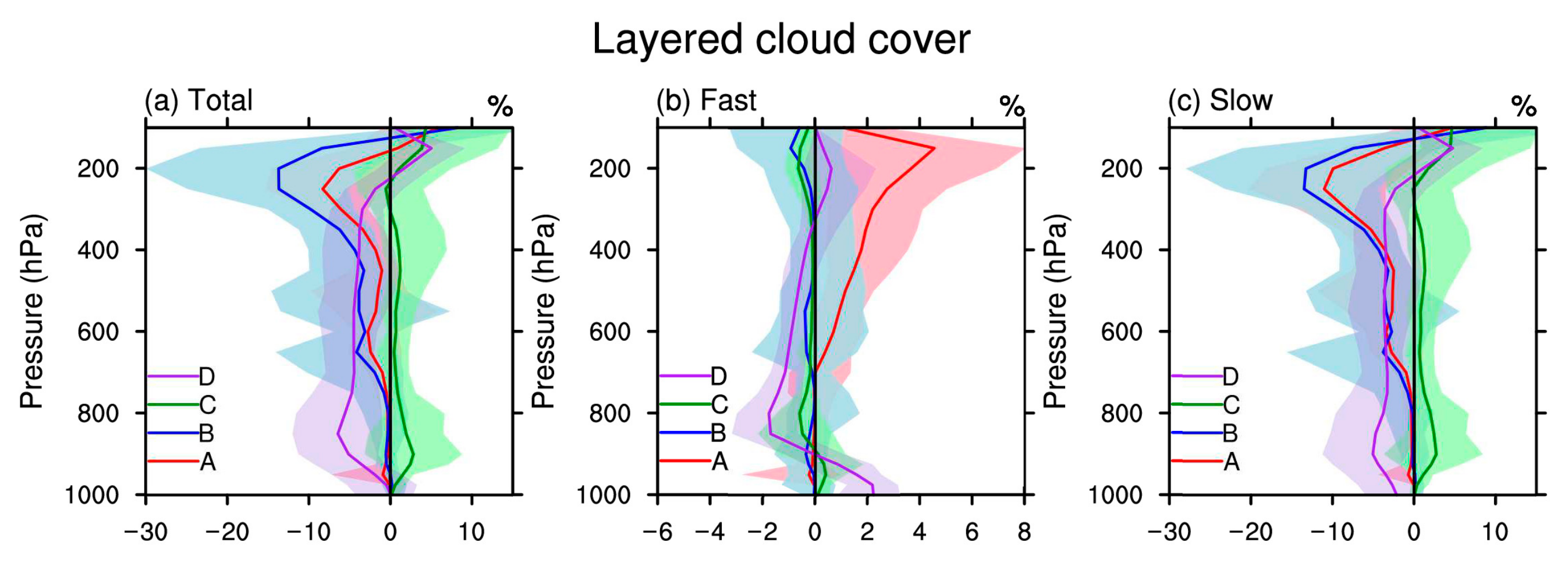
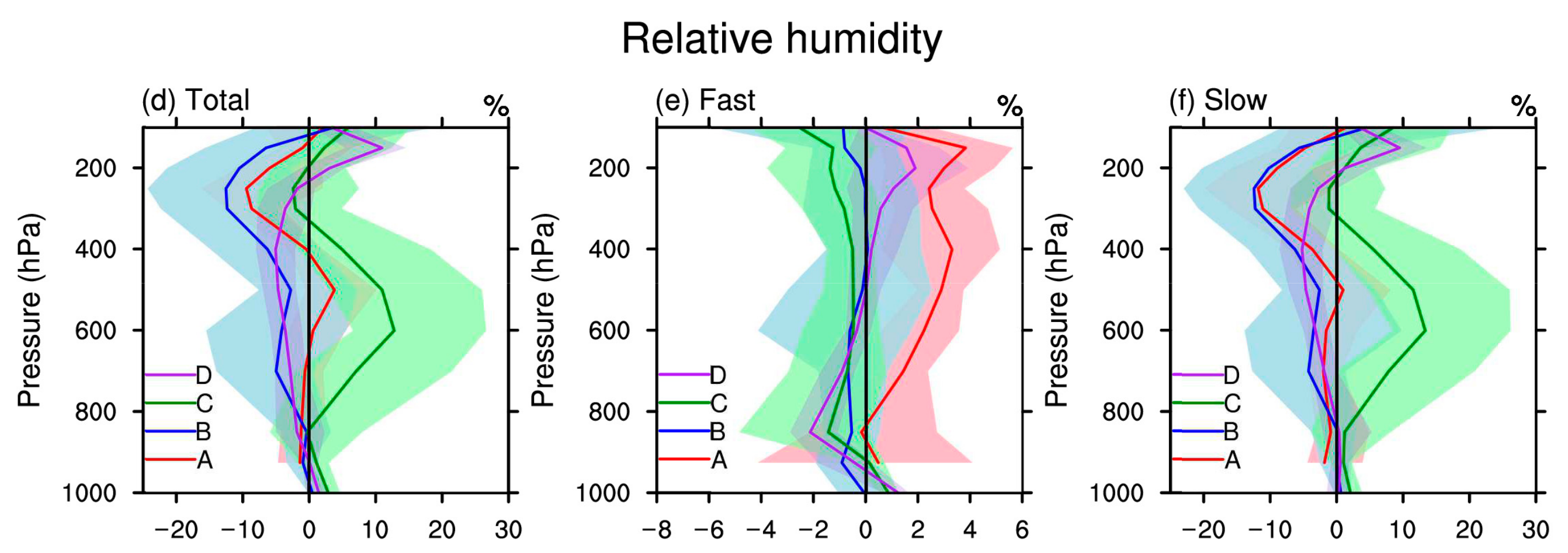
Figure 11a–c shows the profiles of the average layered cloud cover changes in four typical regions. In the total and the slow responses, cloud cover decreases from surface to high altitude in regions A and B with a minimum reaching around 250 hPa, while an opposite trend is demonstrated in region C. The cloud cover profile shows more complex changes for region D, with a decreasing trend from the surface to about 220 hPa and transforming to an increasing trend in the upper atmosphere. In the fast response, cloud cover increases significantly at 700–100 hPa with a maximum reaching 150 hPa in region A, while it decreases slightly in all layers for regions B and C. The cloud cover in region D increases from surface to 900 hPa and at pressures less than 300 hPa in the upper atmosphere, but decreases at 900–300 hPa. Figure 11d–f shows the profiles of average RH changes in four typical regions. In short, the change in the RH is generally consistent with the change in layered cloud cover. However, in the total and slow responses, the RH in region C increases significantly in the middle atmosphere at 800–400 hPa, but with slight changes in the layered cloud cover. This is largely different from the remarked TCC increases over this region (Figure 2 and Table 2), suggesting that the multi-models’ representation of a layered cloud cover is not sufficient in this region.
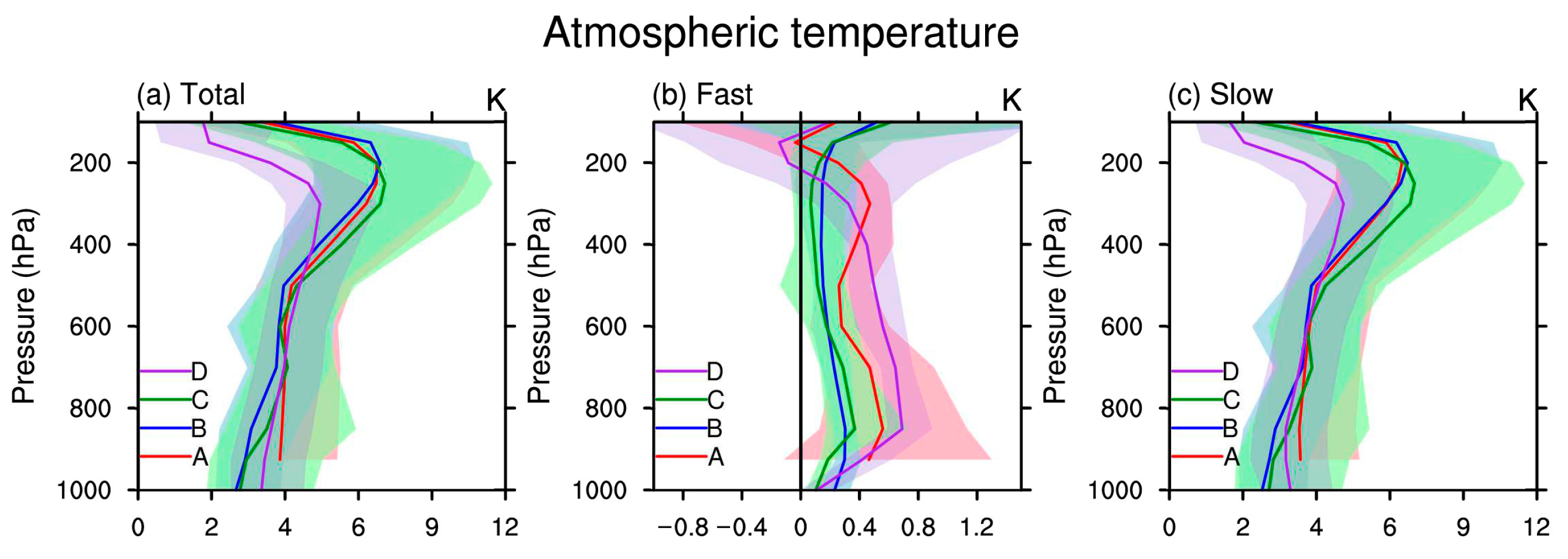
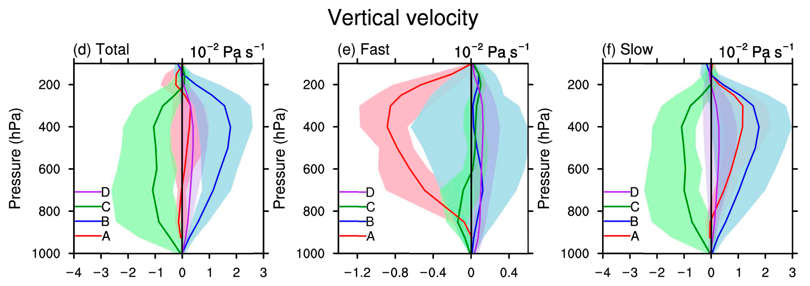
Figure 12 represents profiles of the average atmospheric temperature and vertical velocity changes in the four typical regions, where positive and negative values of the vertical velocity represent anomalous descending and ascending motions, respectively. In the total and slow responses, the vertical velocities mainly demonstrate positive anomalies in regions A and B, which indicate the descending motion anomalies in these two regions, resulting in a decrease in TCC. In particular, the significant increases in the upper atmospheric temperature in these two regions greatly increase the saturation water vapor pressure, resulting in a remarked decrease in high cloud cover. The negative anomalies of vertical velocity occur in region C and the positive anomalies occur in region D in the total and the slow responses, which leads to an increase and a decrease in TCC in regions C and D, respectively. In the fast response, the significant negative anomaly of the vertical velocity in region A leads to a remarked increase in TCC, while the positive anomaly of the vertical velocity from the surface to the upper atmosphere in region B contributes to the TCC decrease over this region. In region C, the positive anomaly of the vertical velocity occurs at pressures less than 600 hPa and the negative anomaly occurs from the surface to 600 hPa but with a water vapor diffusion in the lower atmosphere (Figure S2b), resulting in the cloud cover reductions in both the lower and upper atmosphere and causing a TCC decrease over this region. In region D, the positive anomaly of the vertical velocity occurs in the whole atmosphere, and this anomalous descending motion leads to a decrease in cloud cover at 900–300 hPa. However, the increase in cloud cover in the upper atmosphere results from the reduction in the saturated water pressure caused by the decrease in the upper atmospheric temperature. In the boundary layer from the surface to 900 hPa, the atmospheric warming increases with the increasing altitudes, which enhances the static stability and accumulates water vapor near the surface, leading to an increase in boundary layer clouds.
4. Conclusions
In this work, the global cloud responses to the quadrupled CO2 forcing are investigated by decomposing the total response into the fast and slow ones using 10 typical model outputs in CMIP6. The major conclusions are as follows.
First, from the modelling year 121 to year 150 after the quadrupling of the CO2 forcing, i.e., the year of the model arriving at quasi-equilibrium after the interruption, the global mean changes of TCC in the total, fast, and slow responses are −2.42%, −0.64%, and −1.78%, respectively. The slow response dominates in most areas, demonstrating similar spatial distributions with the total response.
Second, the changes in cloud cover are mainly determined by the vertical motion and atmospheric temperature changes. The change in vertical motion is the major contributor to the cloud cover change at middle and low latitudes, while the decrease in upper atmospheric temperature leads to an increase in high cloud cover at high latitudes. In addition, the water vapor convergence/diffusion anomaly also contributes to the increase/decrease in cloud cover at low latitudes.
Third, four typical regions are selected for the detailed analysis, and the result suggests that slow responses also dominate regional cloud changes, and changes in vertical motion and atmospheric temperature are critical to regional cloud changes.
Supplementary Materials
The following supporting information can be downloaded at: https://www.mdpi.com/article/10.3390/atmos14040653/s1, Table S1: The 44 models used to calculate the total response and the 12 models used to calculate the fast response in Figure S1; Table S2: The 9 models used to calculate the convective cloud cover in Figure S2; Figure S1: (a) The total response of TCC from 44 available models and (b) the fast response from 12 available models; Figure S2: (a) The distribution of convective cloud cover provided by 9 available models in piControl and (b) the difference between abrupt-4xCO2 and piControl; Figure S3: (a) Total, (b) fast, and (c) slow responses of global vertical integrated column horizontal water vapor flux and divergence from 1000 hPa to 680 hPa; Figure S4: Same as Figure S3, but from 680 hPa to 440 hPa; Figure S5: Same as Figure S3, but from 440 hPa to 100 hPa; Figure S6: (a) Total, (b) fast, and (c) slow responses of 500 hPa relative humidity.
Author Contributions
Conceptualization, X.Z., H.Z. and B.X.; methodology, X.Z. and B.X.; validation, Q.W. and B.X.; formal analysis, X.Z.; investigation, X.Z.; data curation, X.Z.; writing—original draft preparation, X.Z.; writing—review and editing, H.Z. and Q.W; visualization, X.Z.; supervision, H.Z.; project administration, H.Z.; funding acquisition, H.Z. All authors have read and agreed to the published version of the manuscript.
Funding
This research was funded by the National Natural Science Foundation of China (grant numbers 42275039 & 41905081), the National Key Research and Development Program of China (grant number 2017YFA0603502), and S&T Development Fund of Chinese Academy of Meteorological Sciences (grant numbers 2021KJ004 & 2022KJ019).
Institutional Review Board Statement
Not applicable.
Informed Consent Statement
Not applicable.
Data Availability Statement
The CMIP data are available through ESGF’s website at https://esgf-node.llnl.gov/projects/cmip6/ (accessed on 29 March 2023).
Acknowledgments
We appreciate two anonymous reviewers for their constructive comments and suggestions.
Conflicts of Interest
The authors declare no conflict of interest.
References
- Liou, K.N. Radiation and Cloud Processes in the Atmosphere; Oxford University Press: New York, NY, USA; Oxford, UK, 1992; pp. 172–248. [Google Scholar]
- Zhang, H.; Jing, X.W.; Peng, J. Cloud Radiation and Climate; China Meteorological Press: Beijing, China, 2019; 270p. (In Chinese) [Google Scholar]
- Zhang, H.; Wang, F.; Zhao, S.Y.; Xie, B. Earth’s energy budget, climate feedbacks, and climate sensitivity. Clim. Chang. Res. 2021, 17, 691–698. (In Chinese) [Google Scholar]
- Ramanathan, V.; Cess, R.D.; Harrison, E.F.; Minnis, P.; Barkstrom, B.R.; Ahmad, E.; Hartmann, D. Cloud-radiative forcing and climate: Results from the earth radiation budget experiment. Science 1989, 243, 57–63. [Google Scholar] [CrossRef] [PubMed] [Green Version]
- Randall, D.A.; Coakley, J.A., Jr.; Fairall, C.W.; Kropfli, R.A.; Lenschow, D.H. Outlook for research on subtropical marine stratiform clouds. Bull. Amer. Meteorol. Soc. 1984, 65, 1290–1301. [Google Scholar] [CrossRef]
- Wielicki, B.A.; Cess, R.D.; King, M.D.; Randall, D.A.; Harrison, E.F. Mission to planet earth: Role of clouds and radiation in climate. Bull. Am. Meteorol. Soc. 1995, 76, 2125–2154. [Google Scholar] [CrossRef]
- Colman, R. A comparison of climate feedbacks in general circulation models. Clim. Dyn. 2003, 20, 865–873. [Google Scholar] [CrossRef]
- Potter, G.L.; Cess, R.D. Testing the impact of clouds on the radiation budgets of 19 atmospheric general circulation models. J. Geophys. Res. 2004, 109, D02106. [Google Scholar] [CrossRef] [Green Version]
- Randall, D.A.; Wood, R.A.; Bony, S.; Colman, R.; Fichefet, T.; Fyfe, J.; Kattsov, V.; Pitman, A.; Shukla, J.; Srinivasan, J.; et al. Cilmate Models and Their Evaluation. In Climate Change 2007: The Physical Science Basis; Contribution of Working Group I to the Fourth Assessment Report of the Intergovernmental Panel on Climate Change; Solomon, S., Qin, D., Manning, M., Chen, Z., Marquis, M., Averyt, K.B., Tignor, M., Miller, H.L., Eds.; Cambridge University Press: Cambridge, UK; New York, NY, USA, 2007; pp. 589–662. [Google Scholar]
- Zhang, H.; Wang, F.; Wang, F.; Li, J.D.; Chen, X.L.; Wang, Z.Z.; Li, J.; Zhou, X.X.; Wang, Q.Y.; Wang, H.B.; et al. Advances in cloud radiative feedbacks in global climate change. Sci. Sin. Terrae 2022, 52, 400–417. (In Chinese) [Google Scholar] [CrossRef]
- Ding, S.G.; Zhao, C.S.; Shi, G.Y.; Wu, C.A. Analysis of global total cloud amount variation over the past 20 years. J. Appl. Meteorol. Sci. 2005, 16, 670–677. [Google Scholar] [CrossRef]
- Norris, J.R. Multidecadal changes in near-global cloud cover and estimated cloud cover radiative forcing. J. Geophys. Res. 2005, 110, D08206. [Google Scholar] [CrossRef]
- Wylie, D.; Jackson, D.L.; Menzel, W.P.; Bates, J.J. Trends in global cloud cover in two decades of HIRS observations. J. Clim. 2005, 18, 3021–3031. [Google Scholar] [CrossRef]
- Liu, Y.H.; Key, J.R.; Wang, X.J. The influence of changes in cloud cover on recent surface temperature trends in the Arctic. J. Clim. 2008, 21, 705–715. [Google Scholar] [CrossRef]
- Sun, B.M.; Free, M.; Yoo, H.L.; Foster, M.J.; Heidinger, A.; Karlsson, K.-G. Variability and trends in U.S. cloud cover: ISCCP, PATMOS-x, and CLARA-A1 compared to homogeneity-adjusted weather observations. J. Clim. 2015, 28, 4373–4389. [Google Scholar] [CrossRef]
- Norris, J.R.; Allen, R.J.; Evan, A.T.; Zelinka, M.D.; O’Dell, C.W.; Klein, S.A. Evidence for climate change in the satellite cloud record. Nature 2016, 536, 72–75. [Google Scholar] [CrossRef] [PubMed] [Green Version]
- Zhou, X.X.; Zhang, H.; Jing, X.W. Distribution and variation trends of cloud amount and optical thickness over China. J. Atmos. Environ. Opt. 2016, 11, 1–13. (In Chinese) [Google Scholar]
- Miller, R.L. Tropical thermostats and low cloud cover. J. Clim. 1997, 10, 409–440. [Google Scholar] [CrossRef]
- Dai, A.G.; Wigley, T.M.L.; Boville, B.A.; Kiehl, J.T.; Buja, L.E. Climates of the twentieth and twenty-first centuries simulated by the NCAR climate system model. J. Clim. 2001, 14, 485–519. [Google Scholar] [CrossRef]
- Vavrus, S. The impact of cloud feedbacks on Arctic climate under greenhouse forcing. J. Clim. 2004, 17, 603–615. [Google Scholar] [CrossRef]
- Bretherton, C.S.; Blossey, P.N. Low cloud reduction in a greenhouse-warmed climate: Results from Lagrangian LES of a subtropical marine cloudiness transition. J. Adv. Model. Earth Syst. 2014, 6, 91–114. [Google Scholar] [CrossRef]
- Wetherald, R.T. The role of low clouds in determining climate sensitivity in response to a doubling of CO2 as obtained from 16 mixed-layer models. Clim. Chang. 2011, 109, 569–582. [Google Scholar] [CrossRef]
- Gregory, J.M.; Ingram, W.J.; Palmer, M.A.; Jones, G.S.; Stott, P.A.; Thorpe, R.B.; Lowe, J.A.; Johns, T.C.; Williams, K.D. A new method for diagnosing radiative forcing and climate sensitivity. Geophys. Res. Lett. 2004, 31, L03205. [Google Scholar] [CrossRef] [Green Version]
- Andrews, T.; Forster, P.M. The transient response of global-mean precipitation to increasing carbon dioxide levels. Environ. Res. Lett. 2010, 5, 025212. [Google Scholar] [CrossRef]
- Bala, G.; Caldeira, K.; Nemani, R. Fast versus slow response in climate change: Implications for the global hydrological cycle. Clim. Dyn. 2010, 35, 423–434. [Google Scholar] [CrossRef]
- Hansen, J.; Sato, M.; Ruedy, R.; Nazarenko, L.; Lacis, A.; Schmidt, G.A.; Russell, G.; Aleinov, I.; Bauer, M.; Bauer, S.; et al. Efficacy of climate forcings. J. Geophys. Res. 2005, 110, D18104. [Google Scholar] [CrossRef]
- Ganguly, D.; Rasch, P.J.; Wang, H.L.; Yoon, J.H. Fast and slow responses of the south Asian monsoon system to anthropogenic aerosols. Geophys. Res. Lett. 2012, 39, L18804. [Google Scholar] [CrossRef]
- Samset, B.H.; Myhre, G.; Forster, P.M.; Hodnebrog, Ø.; Andrews, T.; Faluvegi, G.; Fläschner, D.; Kasoar, M.; Kharin, V.; Kirkevåg, A.; et al. Fast and slow precipitation responses to individual climate forcers: A PDRMIP multimodel study. Geophys. Res. Lett. 2016, 43, 2782–2791. [Google Scholar] [CrossRef] [Green Version]
- Wang, Z.L.; Lin, L.; Yang, M.L.; Xu, Y.Y.; Li, J.N. Disentangling fast and slow responses of the east Asian summer monsoon to reflecting and absorbing aerosol forcings. Atmos. Chem. Phys. 2017, 17, 11075–11088. [Google Scholar] [CrossRef] [Green Version]
- Duan, L.; Cao, L.; Bala, G.; Calderia, K. Comparison of the fast and slow climate response to three radiation management geoengineering schemes. J. Geophys. Res. 2018, 123, 11980–12001. [Google Scholar] [CrossRef]
- Hansen, J.; Sato, M.; Simons, L.; Nazarenko, L.S.; von Schuckmann, K.; Loeb, N.G.; Osman, M.B.; Kharecha, P.; Jin, Q.J.; Tselioudis, G.; et al. Global warming in the pipeline. arXiv 2022. [Google Scholar] [CrossRef]
- Gregory, J.M.; Webb, M. Tropospheric adjustment induces a cloud component in CO2 forcing. J. Clim. 2008, 21, 58–71. [Google Scholar] [CrossRef]
- Kamae, Y.; Watanabe, M. On the robustness of tropospheric adjustment in CMIP5 models. Geophys. Res. Lett. 2012, 39, L23808. [Google Scholar] [CrossRef]
- Webb, M.J.; Lambert, F.H.; Gregory, J.M. Origins of differences in climate sensitivity, forcing and feedback in climate models. Clim. Dyn. 2013, 40, 677–707. [Google Scholar] [CrossRef]
- Kamae, Y.; Watanabe, M.; Ogura, T.; Yoshimori, M.; Shiogama, H. Rapid adjustments of cloud and hydrological cycle to increasing CO2: A review. Curr. Clim. Chang. Rep. 2015, 1, 103–113. [Google Scholar] [CrossRef] [Green Version]
- Dinh, T.; Fueglistaler, S. On the Causal Relationship Between the Moist Diabatic Circulation and Cloud Rapid Adjustment to Increasing CO2. J. Adv. Model. Earth Syst. 2019, 11, 3836–3851. [Google Scholar] [CrossRef] [Green Version]
- Wyant, M.C.; Bretherton, C.S.; Blossey, P.N.; Khairoutdinov, M. Fast cloud adjustment to increasing CO2 in a superparameterized climate model. J. Adv. Model. Earth Syst. 2012, 4, M05001. [Google Scholar] [CrossRef]
- Xu, K.M.; Li, Z.; Cheng, A.; Hu, Y. Changes in clouds and atmospheric circulation associated with rapid adjustment induced by increased atmospheric CO2: A multiscale modeling framework study. Clim. Dyn. 2020, 55, 277–293. [Google Scholar] [CrossRef] [Green Version]
- Dong, B.; Gregory, J.M.; Sutton, R.T. Understanding land–sea warming contrast in response to increasing greenhouse gases. Part I: Transient adjustment. J. Clim. 2009, 22, 3079–3097. [Google Scholar] [CrossRef]
- Zelinka, M.D.; Klein, S.A.; Taylor, K.E.; Andrews, T.; Webb, M.J.; Gregory, J.M.; Forster, P.M. Contributions of different cloud types to feedbacks and rapid adjustments in CMIP5. J. Clim. 2013, 26, 5007–5027. [Google Scholar] [CrossRef] [Green Version]
- Andrews, T.; Ringer, M.A. Cloud feedbacks, rapid adjustments, and the forcing–response relationship in a transient CO2 reversibility scenario. J. Clim. 2014, 27, 1799–1818. [Google Scholar] [CrossRef]
- Zhou, X.X.; Xie, B.; Zhang, H.; He, J.Y.; Chen, Q. Decomposition of fast and slow cloud responses to quadrupled CO2 forcing in BCC–AGCM2.0 over East Asia. Adv. Atmos. Sci. 2022, 39, 2188–2202. [Google Scholar] [CrossRef]
- Eyring, V.; Bony, S.; Meehl, G.A.; Senior, C.A.; Stevens, B.; Stouffer, R.J.; Taylor, K.E. Overview of the coupled model intercomparison project phase 6 (CMIP6) experimental design and organization. Geosci. Model Dev. 2016, 9, 1937–1958. [Google Scholar] [CrossRef] [Green Version]
- Serreze, M.C.; Barry, R.G. Processes and impacts of Arctic amplification: A research synthesis. Global Planet. Chang. 2011, 77, 85–96. [Google Scholar] [CrossRef]
- Li, J.D.; You, Q.L.; He, B. Distinctive spring shortwave cloud radiative effect and its inter-annual variation over southeastern China. Atmos. Sci. Lett. 2020, 21, e970. [Google Scholar] [CrossRef] [Green Version]
Figure 1.
(a) Total, (b) fast, and (c) slow responses of global surface air temperature (units: K). Black dot represents that at least 8 models agree with the sign of changes.
Figure 1.
(a) Total, (b) fast, and (c) slow responses of global surface air temperature (units: K). Black dot represents that at least 8 models agree with the sign of changes.

Figure 2.
(a) Total, (b) fast, and (c) slow responses of global total cloud cover (units: %). Black dot represents that at least 8 models agree with the sign of changes.
Figure 2.
(a) Total, (b) fast, and (c) slow responses of global total cloud cover (units: %). Black dot represents that at least 8 models agree with the sign of changes.

Figure 3.
Zonal mean responses of the global total cloud cover (units: %). The red, blue, and green lines represent the total, fast, and slow responses, respectively. The shadows show the maximum and minimum values of the 10 models.
Figure 3.
Zonal mean responses of the global total cloud cover (units: %). The red, blue, and green lines represent the total, fast, and slow responses, respectively. The shadows show the maximum and minimum values of the 10 models.

Figure 4.
Responses of the global mean total cloud cover in 10 typical models (units: %). The red, blue, and green columns represent the total, fast, and slow responses, respectively, and the dotted lines represent the multi-model mean values.
Figure 4.
Responses of the global mean total cloud cover in 10 typical models (units: %). The red, blue, and green columns represent the total, fast, and slow responses, respectively, and the dotted lines represent the multi-model mean values.

Figure 5.
Regions with TCC changes dominated by the fast (blue) and slow response (pink), respectively. Black dot represents that at least 8 models agree with the sign of changes.
Figure 5.
Regions with TCC changes dominated by the fast (blue) and slow response (pink), respectively. Black dot represents that at least 8 models agree with the sign of changes.

Figure 6.
(a) Total, (b) fast, and (c) slow responses of global zonal mean layered cloud cover (units: %). Black dot represents that at least 8 models agree with the sign of changes.
Figure 6.
(a) Total, (b) fast, and (c) slow responses of global zonal mean layered cloud cover (units: %). Black dot represents that at least 8 models agree with the sign of changes.

Figure 7.
(a) Total, (b) fast, and (c) slow responses of global vertical velocity at 500 hPa (ω500, units: 10−2 Pa s−1). Black dot represents that at least 8 models agree with the sign of changes.
Figure 7.
(a) Total, (b) fast, and (c) slow responses of global vertical velocity at 500 hPa (ω500, units: 10−2 Pa s−1). Black dot represents that at least 8 models agree with the sign of changes.

Figure 8.
(a) Total, (b) fast, and (c) slow responses of global vertical integrated column horizontal water vapor flux (QF, vector, and units: kg m−1 s−1) and divergence (QD, colour shading, units: 10−5 kg m−2 s−1; positive values represent water vapor diffusion).
Figure 8.
(a) Total, (b) fast, and (c) slow responses of global vertical integrated column horizontal water vapor flux (QF, vector, and units: kg m−1 s−1) and divergence (QD, colour shading, units: 10−5 kg m−2 s−1; positive values represent water vapor diffusion).

Figure 9.
(a) Total, (b) fast, and (c) slow responses of global zonal mean relative humidity (units: %). Black dot represents that at least 8 models agree with the sign of changes.
Figure 9.
(a) Total, (b) fast, and (c) slow responses of global zonal mean relative humidity (units: %). Black dot represents that at least 8 models agree with the sign of changes.

Figure 10.
(a,d) Total, (b,e) fast, and (c,f) slow responses of global zonal mean (a–c) atmospheric temperature (unit: K) and (d–f) vertical velocity (unit: 10−2 Pa s−1). Black dot represents that at least 8 models agree with the sign of changes.
Figure 10.
(a,d) Total, (b,e) fast, and (c,f) slow responses of global zonal mean (a–c) atmospheric temperature (unit: K) and (d–f) vertical velocity (unit: 10−2 Pa s−1). Black dot represents that at least 8 models agree with the sign of changes.

Figure 11.
(a,d) Total, (b,e) fast, and (c,f) slow responses of (a–c) layered cloud cover (unit: %) and (d–f) relative humidity (unit: %) in four typical regions. The red, blue, green, and purple lines represent regions A, B, C, and D, respectively.
Figure 11.
(a,d) Total, (b,e) fast, and (c,f) slow responses of (a–c) layered cloud cover (unit: %) and (d–f) relative humidity (unit: %) in four typical regions. The red, blue, green, and purple lines represent regions A, B, C, and D, respectively.


Figure 12.
(a,d) Total, (b,e) fast, and (c,f) slow responses of (a–c) atmospheric temperature (unit: K) and (d–f) vertical velocity (unit: 10−2 Pa s−1) in four typical regions. The red, blue, green, and purple lines represent regions A, B, C, and D, respectively.
Figure 12.
(a,d) Total, (b,e) fast, and (c,f) slow responses of (a–c) atmospheric temperature (unit: K) and (d–f) vertical velocity (unit: 10−2 Pa s−1) in four typical regions. The red, blue, green, and purple lines represent regions A, B, C, and D, respectively.


Table 1.
CMIP6 models used in this study.
| Model Name | Institution | Nation | Resolution (Longitude × Latitude) |
|---|---|---|---|
| ACCESS-CM2 | CSIRO-ARCCSS | Australia | 1.875° × 1.25° |
| ACCESS-ESM1-5 | CSIRO | Australia | 1.875° × 1.25° |
| CESM2 | NCAR | USA | 1.25° × 0.9375° |
| GISS-E2-1-G | NASA-GISS | USA | 2.5° × 2° |
| IPSL-CM6A-LR | IPSL | France | 2.5° × 1.25° |
| MIROC6 | MIROC | Japan | 1.4° × 1.4° |
| MPI-ESM1-2-LR | MPI-M | Germany | 1.875° × 1.875° |
| MRI-ESM2-0 | MRI | Japan | 1.125° × 1.125° |
| NorESM2-LM | NCC | Norway | 2.5° ×1.875° |
| NorESM2-MM | NCC | Norway | 1.25° × 0.9375° |
Table 2.
Mean changes in total cloud cover in the globe and in four typical regions *.
| Global | A | B | C | D | |||||||||||
|---|---|---|---|---|---|---|---|---|---|---|---|---|---|---|---|
| Total | Fast | Slow | Total | Fast | Slow | Total | Fast | Slow | Total | Fast | Slow | Total | Fast | Slow | |
| TCC (%) | −2.42 | −0.64 | −1.78 | −5.12 | 3.01 | −8.13 | −6.76 | −0.82 | −5.94 | 9.95 | −1.14 | 11.09 | −5.95 | 0.44 | −6.39 |
* The geographic ranges of four typical regions are given as follows: A: 15° S–15° N, 15–35° E; B: 10° S–10° N, 100° E–130° E; C: 0–20° S, 130° W–100° W; D: 30° N–50° N, 170° E–160° W.
Disclaimer/Publisher’s Note: The statements, opinions and data contained in all publications are solely those of the individual author(s) and contributor(s) and not of MDPI and/or the editor(s). MDPI and/or the editor(s) disclaim responsibility for any injury to people or property resulting from any ideas, methods, instructions or products referred to in the content. |
© 2023 by the authors. Licensee MDPI, Basel, Switzerland. This article is an open access article distributed under the terms and conditions of the Creative Commons Attribution (CC BY) license (https://creativecommons.org/licenses/by/4.0/).
Share and Cite
MDPI and ACS Style
Zhou, X.; Zhang, H.; Wang, Q.; Xie, B. Decomposing Fast and Slow Responses of Global Cloud Cover to Quadrupled CO2 Forcing in CMIP6 Models. Atmosphere 2023, 14, 653. https://doi.org/10.3390/atmos14040653
AMA Style
Zhou X, Zhang H, Wang Q, Xie B. Decomposing Fast and Slow Responses of Global Cloud Cover to Quadrupled CO2 Forcing in CMIP6 Models. Atmosphere. 2023; 14(4):653. https://doi.org/10.3390/atmos14040653
Chicago/Turabian StyleZhou, Xixun, Hua Zhang, Qiuyan Wang, and Bing Xie. 2023. "Decomposing Fast and Slow Responses of Global Cloud Cover to Quadrupled CO2 Forcing in CMIP6 Models" Atmosphere 14, no. 4: 653. https://doi.org/10.3390/atmos14040653
Note that from the first issue of 2016, this journal uses article numbers instead of page numbers. See further details here.