Article

Filtration Kinetics of Depth Filters—Modeling and Comparison with Tomographic Data of Particle Depositions

1
Department of Applied Life Sciences and Process Engineering, Anhalt University of Applied Science, Bernburger Str. 55, D-06366 Koethen, Germany
2
Laboratory of Solids Process Engineering, Department of Bio- and Chemical Engineering, TU Dortmund University, Emil-Figge Str. 68, D-44227 Dortmund, Germany
3
RIF-Institut für Forschung und Transfer e.V., Joseph-von-Fraunhofer Str. 20, D-44227 Dortmund, Germany
*
Author to whom correspondence should be addressed.
Atmosphere 2023, 14(4), 640; https://doi.org/10.3390/atmos14040640
Submission received: 16 February 2023 / Revised: 21 March 2023 / Accepted: 23 March 2023 / Published: 28 March 2023
(This article belongs to the Section Air Pollution Control)

Abstract

:
Depth filtration is a widespread technique for the separation of airborne particles. The evolution of the pressure difference within this process is determined to a significant extent by the filter structure. Simulations are an important tool for optimizing the filter structure, allowing the development of filter materials having high filtration efficiencies and low pressure differences. Because of the large number of physical phenomena and the complex structure of filter materials, simulations of the filtration kinetics are, however, challenging. In this context, one-dimensional models are advantageous for the calculation of the filtration kinetics of depth filters, due to their low computation requirements. In this work, an approach for combining a one-dimensional model with microstructural data of filter materials is presented. This enables more realistic modeling of the filtration process. Calculations were performed on a macroscopic as well as microscopic level and compared to experimental data. With the suggested approach, the influence of a measured microstructure on the results was examined and predictability was improved. Especially for small research departments and for the development of optimized filter materials adapted to specific separation tasks, this approach provides a valuable tool.

1. Introduction

Numerous studies have confirmed the health-endangering effect of fine dust particles [1,2,3,4,5,6]. Consequently, the emission of these particles must be avoided, or efficient processes are required for the purification of polluted air [6]. Fibrous depth filters are a widely-used method for separating particles and to supply particulate free air in numerous applications [7]. Due to their low investment costs and flexible design, which allows them to be adapted to the operating conditions, depth filters are a key component in, for example ventilation systems [8]. High filtration efficiencies are required, especially for particles classified as particularly hazardous in the size class smaller than 2.5 µm [6]. Depth filters are able to achieve the highest separation rates through high packing densities and small fiber diameters [9,10]. The energy consumption of a ventilation system is largely determined by the power consumption of the fans which have to overcome the pressure difference caused by the flow through the filter [10]. The pressure difference increases during the filtration process as a result of the particulate matter clogging the filter can reach values several times higher than the initial pressure [11]. The pressure difference characteristics during the filtration process are determined by the filter material [12]. To achieve the goals of resource efficiency and sustainability, the increase of the pressure difference should be as low as possible.
This can be realized by adapting filter materials exhibiting a high dust-holding capacity. This is usually connected to a homogenous loading of the entire filter with particles e.g., by an optimized internal gradient porosity [13,14]. Progress in terms of lowering penetration rates and increasing dust holding capacity have been conducted by the use of hybrid filtration processes such as electrostatically assisted air filters [15,16].
However, the filter material structure in most processes was identified as a decisive parameter, and its microstructure particularly has a significant influence on the filtration efficiency and the dust holding capacity. [13,14,17,18] The selection and optimization of suitable filter materials for a given separation task is therefore an important issue when designing depth filter materials [13,14,19].
In recent decades, simulations became a valuable tool, both to support the design of advanced filter materials and to allow a deeper understanding of the mechanism and the kinetics of the filtration process [13,14,18,20,21,22,23,24]. The challenge here is the degree to which the physical processes are represented in the simulations, especially if the kinetics of the filtration are to be considered [25].
Although simulations in 3D and 2D are well developed [26,27], there might be a request for alternative ways to describe and predict filtration behaviors, especially when experimental data—e.g., derived by computer tomography (CT)—can be compared with the model calculations [25].
Due to their low computing requirements, one-dimensional models have been applied to approximate filtration kinetics, i.e., filtration efficiency and pressure difference evolution of depth filter materials, during the filtration process [19,28,29]. While 2D or 3D simulations describe the filtration process by means of the numerical calculation of flow fields within the meshed filter structure, 1D simulations take a different approach [19]. These types of simulations discretize the filter in the axial (flow) direction, along with its depth in individual sub filters [19,28,29]. The fluid dynamics and the particle separation in each of the sub filters are calculated using cell models according to single fiber efficiency theory. Finally, the influence of deposited particles on filtration kinetics is addressed by a dynamically alternating filter structure. In Thomas et al. [19], the pressure difference and filtration efficiency of different filter materials were successfully described, and an optimal association of different filter materials was identified. Moreover, applications to granular filtration materials [30] and the consecutive filtration processes of a liquid and solid aerosol were described [31]. The question that arises is as follows: to what degree is a simplification of the filter properties such as porosity and fiber diameter possible in a one-dimensional view?
However, in most of these calculations, the microstructure of the filter material and the local distribution of accumulated particles inside the filter material were not considered in detail. Although the location of particle deposition within a filter material was quantified via experiments and compared with the modeled prediction in Thomas et al. [28], the influence of microstructures on the calculation and the accuracy of one-dimensional models, at the microstructural level, remains unclear. The aim of this study is to simulate the filtration process using microstructural data of the real filter material. A validation should be performed on the microscopic level considering CT-data (porosity profile) as well as on the macroscopic level using pressure difference.
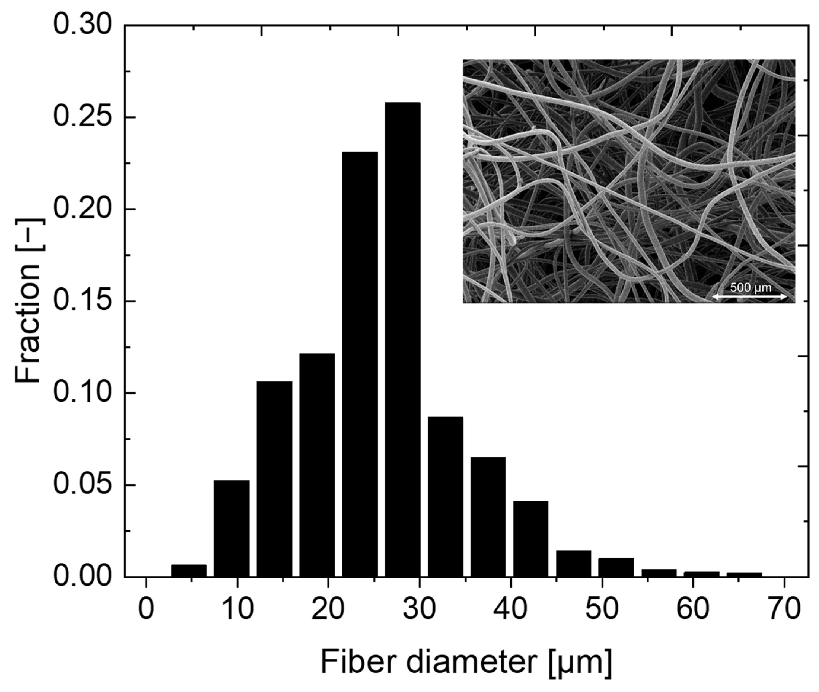
For this purpose, the microstructure of the filter material was imaged using X-ray microscopy (XRM) and applied as an input for the calculation, as described in our previous work [32]. The filter material used for the test case is a typical coarse dust filter, as used in room air cleaners or air conditioning systems as a pre-filter in cascades to relieve downstream high-efficiency filters [33,34]. The model was extended to include the influence of particles deposited during filtration. The aim was to improve prediction of filtration kinetics using a one-dimensional approach by including the filter microstructure. The obtained computed data were compared with experimental data at the macroscopic level based on evolving pressure difference and filtration efficiency with respect to filtration time. At the microscopic level, calculated data were validated in comparison with experimental values based on spatially as well as temporally resolved particle deposition collected via XRM.

2. Approach for Calculating Filtration Kinetics Considering Tomographic Data

The computational effort of simulating filtration kinetics increases with the level of detail of the description of physical phenomena occurring [25]. Due to the low computational effort, one-dimensional modeling is advantageous for calculating filtration in depth filters. The complexity of the model is reduced by only carrying out an axial discretization of the filter, and by describing fluid dynamics via semi-empirical correlations [19].
Despite these simplifications, this approach is able to reproduce the filtration properties of filter materials [19]. However, there are still few data available related to how this type of simulation deals with filter microstructure. In order to explicitly represent the microstructure of a filter material (e.g., a porosity gradient), an approach was presented in previous work in which one-dimensional modeling was combined with tomographic data of the microstructure of two filter materials [32]. However, the approach already presented was limited to the initial state of the filter material. In the following, this approach was taken up again and extended by two methods to account for the influence of the filter loading on the calculated filtration parameters.
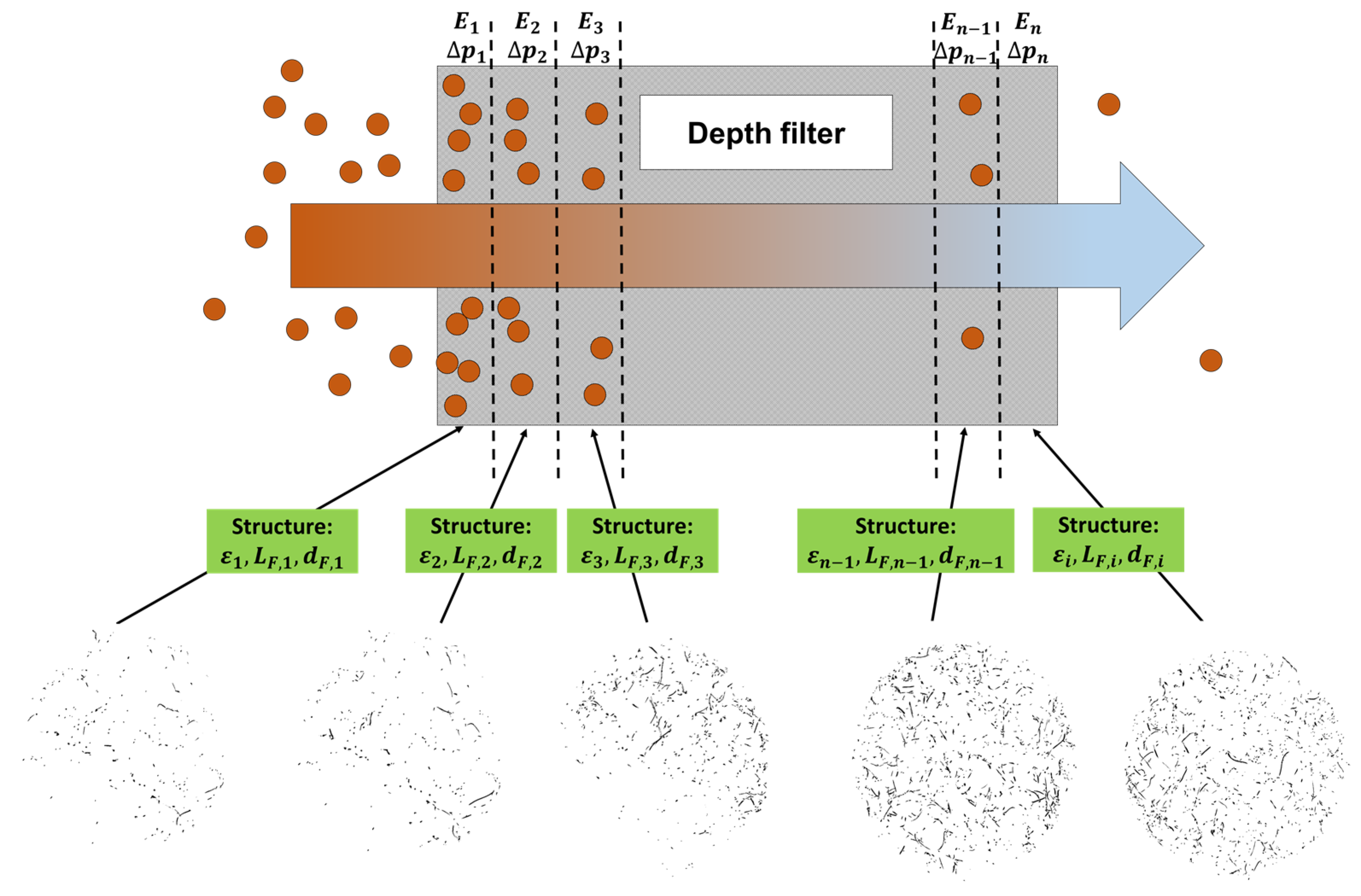
The procedure of the original modeling scheme is visualized in Figure 1. The filter was discretized into a defined number of sub filters ( n ) along the axial flow direction in which calculation of pressure difference and particle deposition takes place. Microstructural properties, such as information about axial resolved porosity, were assigned to each sub filter. In the Figure 1 below, this is represented by sectional images of the filter’s microstructure as provided by tomographic imaging techniques. The number and thickness of the sub filters, having the index i , initially corresponds to those of the axial resolution of the measurement system used.
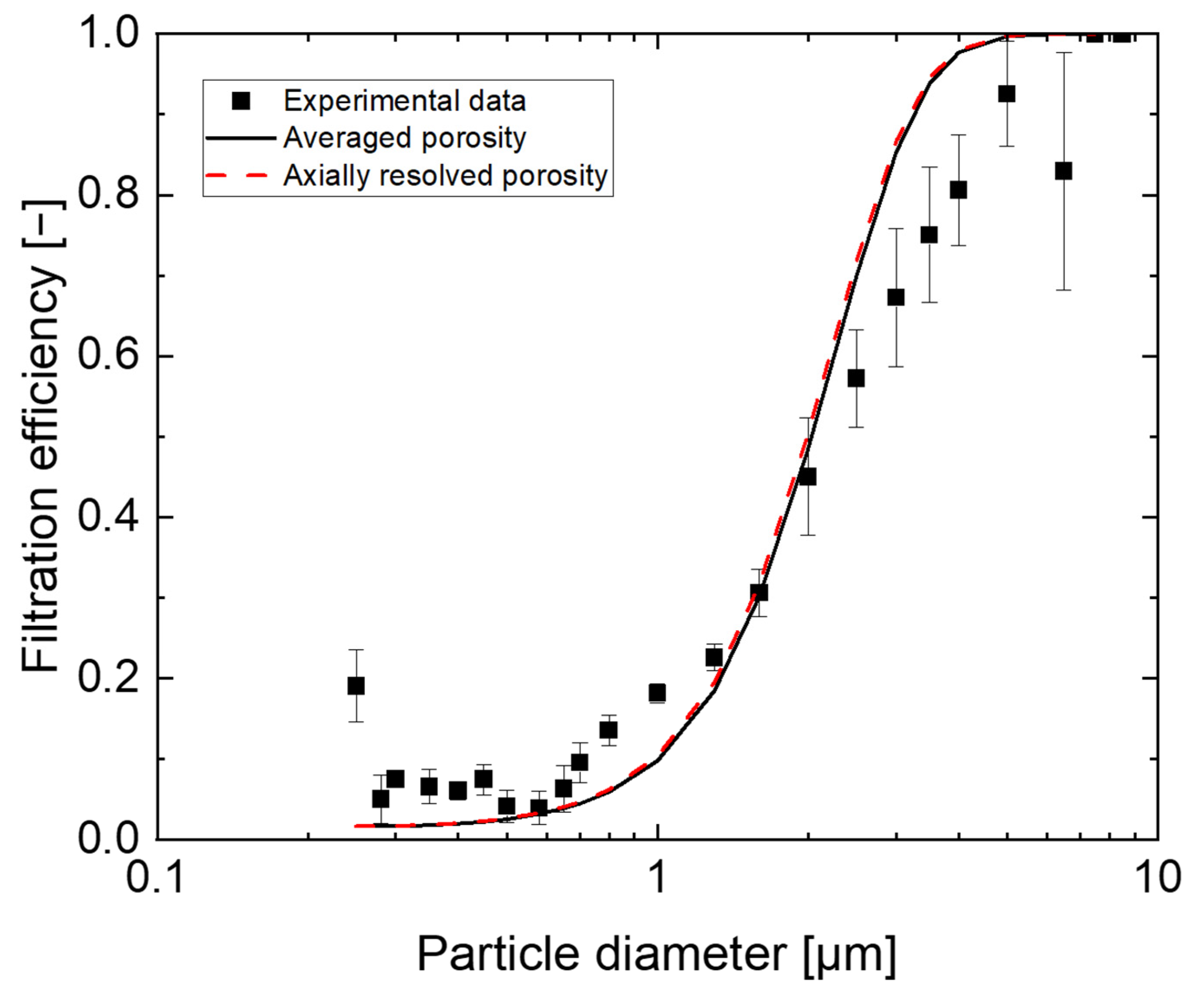
The filtration efficiency ( E i , 0 ) in each subfilter i can be written according to Equation (1), applying the porosity ( ε i ), fiber diameter ( d F , i ) the adhesion coefficient h and filter depth ( L F , i ) of each subfilter.
E i , 0 = 1 exp [ 4 π · ( 1 ε i ε i ) · L F , i d F , i · φ i · h ]
The single fiber efficiency ( φ i ) was expressed by summarizing individual separation efficiencies based on diffusion ( η D + R , i ), inertial effects ( η I , i ), and interception ( η R , i ) (Equation (2)). It must be pointed out that a combination of these effects is responsible for the separation of a particle, and that the sum of individual separation efficiencies cannot exceed the value of 1.
φ i = η D + R , i + η R , i + η I , i
Models used for calculating individual separation mechanisms according to single fiber efficiency theory applied are summarized in Table 1. The fluid dynamics were calculated using the Kuwabara cell model [35].
The diameter distribution of the collectors have a significant influence on the calculation of filtration efficiencies or pressure differences [30,38,39,40,41]. In contrast to the previously discussed approach [32], where the median diameter of the fibers was applied, the distribution of the fiber diameter was utilised here. Filtration efficiencies were calculated for each occurring fiber diameter j according to Equation (1). These were weighted by their fraction in the fiber distribution Δ F i , j according to Equation (3).
E i = j = 1 num   fiber   diameter E i , 0 , j · Δ F i , j
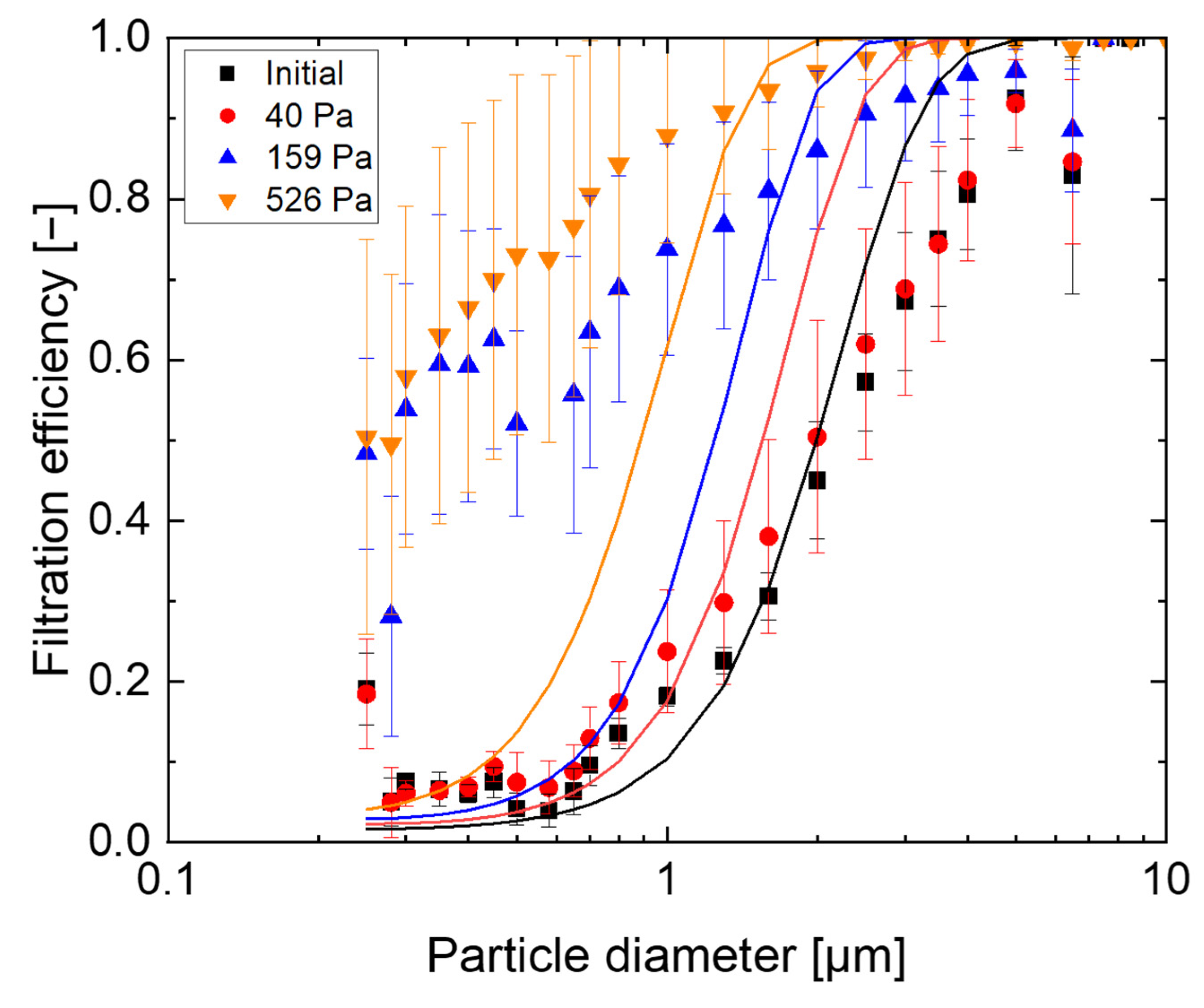
The overall filtration efficiency ( E total ) was computed by summarizing the filtration efficiency of all considered sub filters (Equation (4)). The filtration efficiency can be individually expressed in terms of particle diameter, total mass, or total number.
E total = i = 1 num   subfilter E i
The pressure difference in each sub filter Δ p i , 0 was determined using Davies’ Equation (5) [42]. Calculations were carried out using the packing density ( α = 1 ε i ), and the dynamic viscosity ( μ ) of air at ambient pressure and 25 °C.
Δ p i , 0 L F , i = 64 · μ · u 0 α i 3 2 · ( 1 + 56 · α i 2 ) d F , i 2
The influence of the fiber diameter distribution on the pressure difference was taken into account, analogous to Equation (3). The total pressure difference of the filter material ( Δ p total ) was derived by adding the individual pressure differences of each sub-filter ( Δ p i ).
Δ p i = i = 1 num   fiber   diameter Δ p i , 0 · Δ F i , j
Δ p total = i = 1 num   subfilter Δ p i
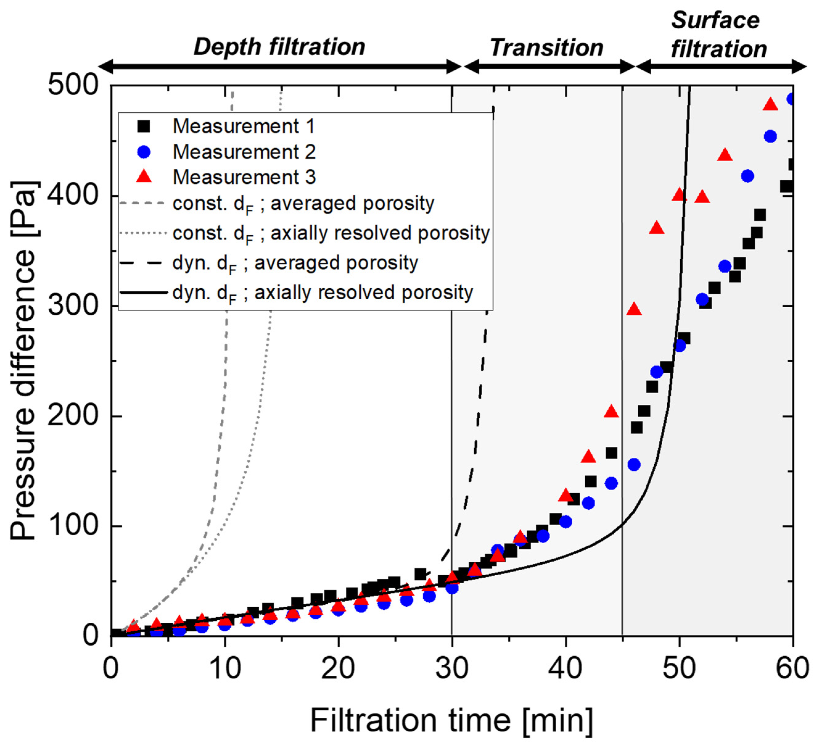
To describe the dynamic change of filtration parameters, such as the pressure difference or filtration efficiency during the filtration process, a change in filter structural properties due to the deposited particles was addressed. First, a decrease in porosity due to the deposition of particles in a sub filter was considered (Equation (8)). For this purpose, the porosity of a sub filter i in the next time step ( ε i , t + 1 ) was re-calculated using the porosity in the current time step ( ε i , t ), the number of particles deposited in sub filter i at the time step t   ( N p , i , t ) and their volume ( V p , i , t calculated assuming ideal spherical particles), as well as the volume of the sub filter i in the initial state of the filter V i , 0 .
ε i , t + 1 = ε i , t i N p , i , t V p , i , t V i , 0
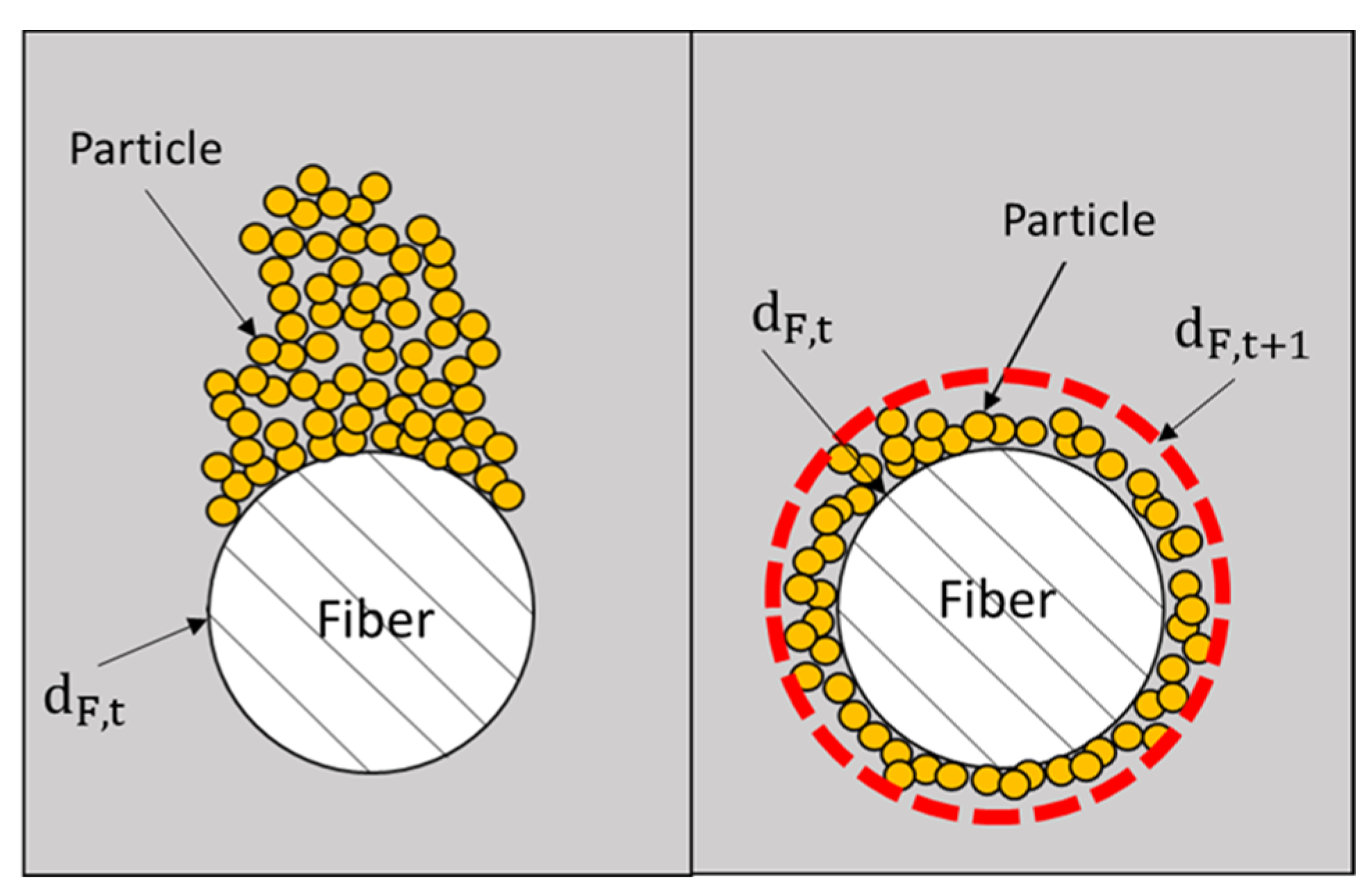
A commonly used approach additionally assumes a constantly increasing fiber diameter d F , i , t + 1 (Figure 2, right) for the next time step (Equation (9)) as for example described in [28,31].
d F , i , t + 1 = 1 ε i , t + 1 1 ε i , t · d F , i , t
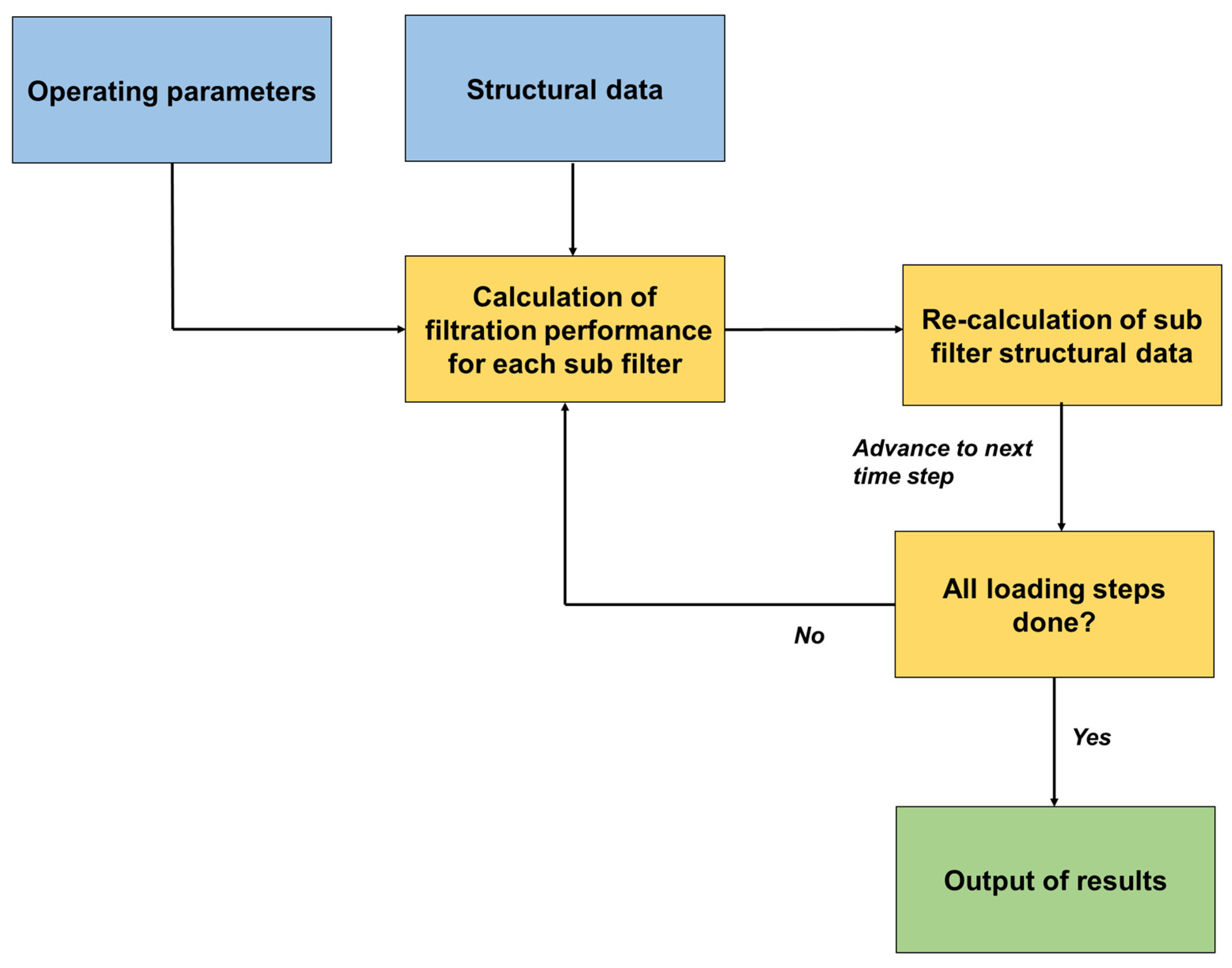
Both presented calculation methods were used to re-calculate the filter structure after each loading step, applying a sequential algorithm illustrated in Figure 3. Calculations of pressure difference and filtration efficiency (Equations (1)–(7)), as well as filter structure (Equations (8) and (9)), were repeated for each considered time step.
The described approach was implemented in MATLAB 2018a (MathWorks Inc., Natick, MA, USA).

3. Results and Discussion

3.1. Application of Modeling Approach

In this chapter, the application of the presented model to a filtration task is discussed. An experimental data set of a previous study was identified as a suitable test case [43]. In this study, experimental data of filtration kinetics of a coarse depth filter were collected during the filtration of a salt aerosol (dp50,3 = 1.5 µm). Therefore, experimental data regarding pressure drop and filtration efficiency, as well as spatially and temporally resolved particle deposition within the filter material during the filtration process, were available. The averaged structural data of the used filter material is given in Table 2.
The operating conditions used in this work are summarized in Table 3. To realize the experimental conditions, particles with a total mass of 347 mg were presented to the filter material within 60 calculation steps representing the filtration time. A filter sample with a cross sectional diameter of 50 mm as used in the experiments was considered in the calculations. Since comparable Stokes numbers of around 0.4 occurred, particle bounce was not incorporated in the calculations. Therefore, the adhesion coefficient (Section 2, Equation (1)) was set to one in all calculations.
A main advantage of the presented approach is the incorporation of the filter microstructure. Therefore, in addition to the averaged porosity, the raw data of the axially resolved porosity, as well as the averaged reference porosity of the clean filter material (Average porosity), are given in Figure 4.
The filter material consisted of a two-stage structure, having a more porous side (>98% porosity) facing the upstream side and a less porous side (<98%) close to the downstream side. The measured microstructure was represented by 1173 porosity measurements in an axial resolution of 12.9 µm. To incorporate this data into the model, an additional modification to the original approach was introduced.
Adjacent porosity data points were combined, and their porosity was averaged, until the thickness of each sub filter reached five times the maximum initial fiber diameter of the fiber diameter distribution. The resulting porosity is given as “axially resolved porosity” in Figure 4. This procedure prevents porosity values connected to a sub filter (Section 2, Figure 1) from having thicknesses smaller than the initial fiber diameter. In addition, by using this procedure, a potential increase of the fiber diameter (Section 2, Equation (9)) due to formation of particle depositions was considered. Even though the resolution of the axial discretization that can be applied in the simulation is diminished from 12.9 µm to 370.4 µm (number of discrete sub filters is reduced from 1173 to 42), the characteristic of the axially resolved porosity could be maintained. Data regarding the number of sub filters and axial resolution were additionally summarized in Table 4.
The fiber diameter distribution of the filter material required for the modeling (Section 2, Equations (3) and (6)) is given in Figure 5. A constant fiber diameter distribution inside the entire filter was assumed for simplification.
A summary of the structural properties of the filter material serving as input is also given in Table 2.
Calculations were performed on a standard desktop PC (Intel(R) Core(TM) i7-4770 CPU @ 3.40 GHz). A complete calculation run was successfully executed within a few minutes.

3.2. Initial Filtration Efficiency

As a first step, computed results were compared with measured data regarding the initial state of the filter material. Figure 6 shows the calculated filtration efficiency of the clean filter material and a comparison with experimental data. Calculations were carried out using the average porosity and the axially resolved porosity as given in Figure 4 of the previous section.
A good agreement was found with respect to experimental data. However, some systematic deviations were noted based on the known inaccuracies of the applied single-fiber models. This might be due to assumed simplifications such as the neglecting of the (radial) heterogenic distribution of the material properties [21,44]. A negligible influence of the axial resolution on the calculation of filtration efficiencies in the initial state was shown, which is in agreement to the results of [17].

3.3. Filtration Kinetics—Macroscopic

In the following, the results of the extended model, including the time-dependent evolution of structural filter properties due to particle deposition, are discussed. Figure 7 shows the comparison between calculated and measured pressure differences, where the pressure is defined as difference between pressure at initial state and current filtration time. All calculations were performed with the same axial discretization (see Section 3.1 Table 4). In separate runs, the sub filters were assigned averaged porosity and axially resolved porosity of the filter material. For both input data, separate calculations were performed assuming a constant fiber diameter (const. d F ) and an increasing fiber diameter (dyn. d F ) during the filtration.
Calculated and experimental results gave a typical progression of the pressure difference. The pressure difference evolution could be divided into depth filtration (filtration time < 30 min), transition (filtration 30 min < time < 45 min), and surface filtration (filtration time > 45 min) zones.
The computed pressure difference increased faster when considering averaged porosity and constant fiber diameter. The decreasing porosity due to the deposited particles within the filter material was responsible for the evolution of the pressure difference and led to an increase of filtration efficiency [9]. The larger fiber diameters occurring within the calculations are less effective in terms of fine particle separation [9,10]. For this reason, assuming an increase in fiber diameter due to particle separation resulted in a slower increase in filtration efficiency. The porosity then decreased more slowly as fewer particles were deposited in the filter, which affected the evolution of the pressure difference.
The selected approach for recalculating the filter structure also had a strong influence even at the beginning of the filtration, while the filter structure led to significant differences at higher filtration times. Therefore, the axial discretization had a more sensitive impact at higher particle loadings of the filter in comparison to the initial state of the filter as also seen in Figure 6.
Calculations incorporating the (measured) axially resolved porosity and an increasing fiber diameter yielded the best results when compared to experimental values of the pressure difference. The pressure difference in depth filtration could be estimated in good agreement with the experimental data; however, deviations between experimental and modeled pressure difference increased with filtration time. The transition and surface filtration state can be reproduced more accurately by applying the axially resolved porosity of the filter material in comparison to the unmodified model (averaged porosity).
However, it must be noted that at higher particle loadings, the assumed simplifications were no longer valid, leading to larger deviations between experimental and modeled data. For longer filtration times, applied models for single fiber efficiency might have exceeded the numerical range they were solved for. Specifically, the expected coalescence of structures, such as bridging of deposited structures at high loading, is not yet incorporated into the approach. It was also shown experimentally that the spatial orientation of the deposits can vary at higher particle loadings [43]. This is not accounted for in the model but might also have an impact on the calculations [22].
In conclusion, the combination of assuming increasing fiber diameter and using axially resolved porosity as the input structure yielded the most promising results with respect to the pressure difference evolution. Therefore, this combination was applied for all further investigations presented.
Figure 8 shows the comparison of the experimental data for filtration efficiencies with the calculated data at different filtration times (pressure differences).
The measured pressure differences at the end of the three identified filtration sections, depth filtration zone (30 min; Δ p = 52 ± 20 Pa), the transition (45 min; Δ p = 168 ± 13 Pa) and the surface filtration zone (60 min; Δ p = 498 ± 25 Pa), were compared with the calculated filtration efficiencies at the computed pressure differences given in the legend of Figure 8. As expected, the experimentally determined and calculated filtration efficiencies increased with higher filter loadings for all particle sizes. For particles in the micrometer range (particle diameter > 1 µm), qualitative agreement between calculated and experimental data could be achieved, but a systematic over-estimation of the particle size must be taken into account, as already noted in Section 3.2. However, the implemented models were not able to reproduce the deposition of particles mainly by diffusion as a function of filtration time/particle loading. It may be necessary to include individual, deposited particles in further work, acting as additional collectors, especially for small particles in the submicron range.

3.4. Filtration Kinetics—Microscopic

The previous results showed that—particularly by applying the (measured) axially resolved microstructure—the estimation of the pressure difference was improved with respect to measurements. In order to evaluate the influence of the microscopic filter media structure, and for deeper insights into the loading behavior of the filters, which are often regarded as a “black box” [45], calculations on a microscopic level were carried out. Figure 9 gives the emerging porosity curves at different loading states calculated assuming increasing fiber diameter. Results are given separately for the averaged (Figure 9, left) and axially resolved porosity (Figure 9, right) as input. Porosity curves were plotted against the dimensionless filter depth, which was defined as the ratio of filter depth to the maximum filter depth, yielding values between 0 and 1. Resulting porosity curves of similar pressure differences during the filtration were compared covering depth, transition, and surface filtration regime.
Areas of low (respectively, decreasing) porosity in the diagrams indicate a strong local accumulation of deposited particles during the filtration process. In the case of an averaged initial porosity (Figure 9, left), particles were predominantly deposited towards the upstream side of the filter. The captured mass within the filter decreased asymptotically towards the downstream side of the filter as indicated by the resulting porosity curve. The particle deposition increased with the filtration time and pressure difference, explained by the additional filtration effect of the deposited particles [28].
A different loading behavior was found by considering the measured microstructure in the calculation. In comparison to the simplified average porosity, two areas of particle accumulations were identified when applying real microstructural data within the calculations (Figure 9, right). In the case of axially resolved porosity, a different microscopic loading behavior was calculated (Figure 9, right). The different microstructure used in the calculations, therefore, strongly affected the presented results. Due to the two-stage structure of the filter material (Figure 4), the local separation efficiency inside the first, more highly porous part of the filter material can change by almost one order of magnitude compared to the less porous stage, close to the downstream side [32]. As a result, particles that penetrated the higher porous part were deposited there, and they gradually formed further collectors in the less porous part. The more homogenous distribution of particles resulted in a more efficient utilization of the entire filter depth for particle storage. This also explained the slower pressure difference increase when applying the axially resolved microstructure in the calculations (Figure 7).
The modeled microscopic particle loading of the filter was qualitatively compared with experimentally obtained 3D images of particle deposition generated using X-ray microscopy (Figure 10). The pressure differences corresponded to experimental values at the end of the depth filtration (Figure 10a), transition (Figure 10b), and surface filtration zones (Figure 10c).
For all three filtration times considered, the axially resolved porosity appeared to provide better agreement as compared to the experimental visualization based on XRM. In the depth filtration zone Figure 10a, the particles were approximately uniformly distributed over the entire filter depth. This behavior could not be reproduced by the model applying averaged porosity as input. Although there is little difference in macroscopic parameters up to filtration times below 30 min (Figure 8), the calculated microscopic loading behavior is different. The differences in microscopic loading behavior, which are comparably small at this filtration time, are negligible when regarding the entirety of the filter.
The calculated, second area showed a significant particle deposition in deeper parts of the filter material close to the downstream side (LF,i/Lmax > 0.7). With the tomographic method, an accumulation of the deposited material was experimentally found in the same zone (Figure 10b,c). Calculations using the averaged porosity as an input parameter showed significant deviations with respect to loading behavior on a microscopic scale in comparison to the visually obtained experimental data. This emphasized the improvement in the calculation of the microscopic loading behavior by this new approach and the suggesting of incorporating the microstructure into one-dimensional calculations as presented herein.
A quantitative comparison of the mass distribution within the filter material is provided in Figure 11. For this purpose, measured and the calculated data were converted into a mass fraction and plotted against the dimensionless filter depth.
Good agreement between experimental and modeled mass distributions was found for all three filtration times considered. However, it was observed that with increasing filter loading (Figure 11b,c), the maximum particle mass shifts to deeper layers compared to lower particle loadings (Figure 11a). The calculated data did not accurately reflect this. One reason considered is the increasing particle load of the filter, which could no longer be described by the models used. Another reason for that behavior might be that, with increasing loading in the experiment, larger particle depositions detached from the fibers because of increasing shear forces and were recaptured in deeper layers. In the analysis of particle deposition applied in Hoppe et al. [43], it was shown that depositions up to six times the size of the fiber diameter were formed, which are more susceptible to shear forces caused by the gas flow due to the larger lever arms. Similar rearrangements or detachments of particles in filter materials or on individual fibers were found, for example, in Jackiewicz et al. [46] or Zoller et al. [47]. In comparison to the experimental values, the calculated values were distributed less widely within the filter materials. This additionally explained the slower increase in the pressure difference in the experiment and gave further indications for the improvement of the modeling approach.

4. Conclusions

In this work, an approach for one-dimensional modeling of the filtration kinetics of depth filters during gas cleaning was presented. In particular, the influence of the microstructure on the performance was investigated. The approach coupled a one-dimensional simulation with high-resolution, structural data of the filter material based on X-ray microscopy. The obtained data were compared with experimental results regarding pressure difference, filtration efficiency, and the positions of particle depositions inside the filter material. Significantly improved agreement with the experimental data of the filtration kinetics was shown compared to calculations that did not incorporate filter microstructure. Improvements were found at the macro and particularly at the microscopic level by the suggested modeling approach. In particular, the microscopic loading behavior of the filter responsible for the pressure difference could be reproduced with the aid of the measured microstructure. This allows the approach to be applied to filter materials of different microstructures and evaluated in terms of their filtration kinetics. Limitations were examined with respect to the prediction of the pressure difference at high filter loadings, as well as the deposition prediction of particles in the submicron range. Due to the low computational effort of only a few minutes on a standard desktop computer, the approach is even suitable as an addition for the selection and optimization of filter structures for customized applications. The presented modeling approach, in combination with experimental methods for analyzing particle deposition at the microscopic level [43], provides multiple options for further research on the dynamic filtration behavior of depth filters.

Author Contributions

Conceptualization, K.H. and D.P.; Investigation, K.H., L.W., G.S. and R.Z.; Software; K.H. and L.W.; Supervision G.S., M.T. and D.P.; Writing-original draft, K.H.; Writing-review and editing, K.H., L.W., G.S., R.Z., W.T., M.T. and D.P. The manuscript was written through contributions of all authors. All authors have read and agreed to the published version of the manuscript.

Funding

We acknowledge support by the German Research Foundation (Deutsche Forschungsgemeinschaft DFG)–project number: 491460386–and the Open Access Publishing Fund of Anhalt University of Applied Sciences for enabling open access publication.

Institutional Review Board Statement

Not applicable.

Informed Consent Statement

Not applicable.

Data Availability Statement

The raw data supporting the conclusion of this article will be made available upon request.

Acknowledgments

The authors are grateful for the assistance of Elizabeth Ely (EIES, Lafayette, IN, USA) in preparing the manuscript.

Conflicts of Interest

The authors declare no conflict of interest.

List of Abbreviations

AbbreviationMeaning
CTComputer tomography
XRMX-ray computed microscopy

List of Latin Symbols

SymbolMeaningUnit
C D , i Correction factor for flow slip for diffusional deposition in subfilter i dimensionless
C D , i Correction factor for diffusional deposition in subilfter i dimensionless
C R , i Correction factor for flow slip for deposition by interception mechanism in subfilter i dimensionless
D Diffusivitym2/s
d F Fiber diameterµm
d F , 50 Mean fiber diameterµm
d F , i Fiber diameter in subfilter i µm
d F , i , t Fiber diameter in subfilter i at loading step tµm
d F , i , t + 1 Fiber diameter in subfilter i at loading step t + 1µm
d p Particle diameterµm
E i Separation efficiency of subfilterdimensionless
E total Total separation efficiency of filterdimensionless
k B Boltzmann constantm2kg/s2K
Kn f , i Knudsen number at the fiber in subfilter i dimensionless
Ku i Kuwabara factor in subfilter i dimensionless
L F , i Depth of subfilter i mm
L F , total Overall depth of filter materialmm
N p , i , t Number of particles deposited in subfilter i at timestep tdimensionless
n i Number of particles in inlet stream of the first subfilterdimensionless
Pe i Peclet-number in subfilter i dimensionless
p i Pressure loss of subfilter ipa
R i Interception parameter in subfilter i dimensionless
Stk i Stokes number in subfilter i dimensionless
T i Separation efficiency of subfilter i dimensionless
u 0 , i gas velocity in subfilter i
u 0 Inlet gas velocitym/s
V i , 0 Free volume of subfilter im3
V p , i , t Volume of particles deposited in subfilter i at loading step tm3

List of Greek Symbols

SymbolMeaningUnit
α Packing densitydimensionless
α i Packing density of subfilter i dimensionless
Δ F i , j Fraction of fiber diameter j in subfilter idimensionless
Δ p i Pressure difference in subfilter ipa
Δ p total Overall pressure difference of filterpa
ε Porositydimensionless
ε av Average porositydimensionless
ε i , t Porosity of subfilter i at timestep tdimensionless
ε i , t + 1 Porosity of subfilter i at timestep t + 1dimensionless
η D + R , i Collection efficiency of single fiber through diffusional and interception mechanism in subfilter i dimensionless
η R , i Collection efficiency of single fiber through interception mechanism in subfilter i dimensionless
η I , i Collection efficiency of single fiber through inertial mechanism in subfilter i dimensionless
ϑ TemperatureK
μ Dynamic viscosity of airPas
ρ p Density of dust particleskg/m3
φ i Single fiber efficiency in subfilter i dimensionless

References

  1. Grantz, D.A.; Garner, J.H.; Johnson, D.W. Ecological effects of particulate matter. Environ. Int. 2003, 29, 213–239. [Google Scholar] [CrossRef] [PubMed]
  2. Kelly, F.J.; Fussell, J.C. Size, source and chemical composition as determinants of toxicity attributable to ambient particulate matter. Atmos. Environ. 2012, 60, 504–526. [Google Scholar] [CrossRef]
  3. Krzyzanowski, M.; Bundeshaus, G.; Negru, M.L.; Salvi, M.C. Particulate Matter Air Pollution: How It Harms Health; World Health Organization: Berlin, Germany; Copenhagen, Denmark; Rome, Italy, 2005; Volume 4, p. 14. [Google Scholar]
  4. Kim, K.-H.; Kabir, E.; Kabir, S. A review on the human health impact of airborne particulate matter. Environ. Int. 2015, 74, 136–143. [Google Scholar] [CrossRef] [PubMed]
  5. Dominici, F.; Greenstone, M.; Sunstein, C.R. Particulate matter matters. Science 2014, 344, 257–259. [Google Scholar] [CrossRef] [Green Version]
  6. Burns, J.; Boogaard, H.; Polus, S.; Pfadenhauer, L.M.; Rohwer, A.C.; van Erp, A.M.; Turley, R.; Rehfuess, E. Interventions to reduce ambient particulate matter air pollution and their effect on health. Cochrane Database Syst. Rev. 2019. [Google Scholar] [CrossRef]
  7. Hinds, W.C.; Zhu, Y. Aerosol Technology: Properties, Behavior, and Measurement of Airborne Particles; John Wiley & Sons: Hoboken, NJ, USA, 2022; ISBN 1119494044. [Google Scholar]
  8. Santos, H.R.; Leal, V.M. Energy vs. ventilation rate in buildings: A comprehensive scenario-based assessment in the European context. Energy Build. 2012, 54, 111–121. [Google Scholar] [CrossRef]
  9. Payen, J.; Vroman, P.; Lewandowski, M.; Perwuelz, A.; Calle-Chazelet, S.; Thomas, D. Influence of fiber diameter, fiber combinations and solid volume fraction on air filtration properties in nonwovens. Text. Res. J. 2012, 82, 1948–1959. [Google Scholar] [CrossRef]
  10. Wang, J.; Kim, S.C.; Pui, D.Y.H. Figure of Merit of Composite Filters with Micrometer and Nanometer Fibers. Aerosol Sci. Technol. 2008, 42, 722–728. [Google Scholar] [CrossRef]
  11. Wang, Q.; Lin, X.; Chen, D.-R. Effect of dust loading rate on the loading characteristics of high efficiency filter media. Powder Technol. 2016, 287, 20–28. [Google Scholar] [CrossRef]
  12. Zhang, W.; Deng, S.; Zhang, S.; Yang, Z.; Lin, Z. Energy consumption performance optimization of PTFE HEPA filter media during dust loading through compositing them with the efficient filter medium. Sustain. Cities Soc. 2022, 78, 103657. [Google Scholar] [CrossRef]
  13. Geerling, C.; Azimian, M.; Wiegmann, A.; Briesen, H.; Kuhn, M. Designing optimally-graded depth filter media using a novel multiscale method. AIChE J. 2020, 66, e16808. [Google Scholar] [CrossRef] [Green Version]
  14. Azimian, M.; Kühnle, C.; Wiegmann, A. Design and optimization of fibrous filter media using lifetime multipass simulations. Chem. Eng. Technol. 2018, 41, 928–935. [Google Scholar] [CrossRef]
  15. Gao, Y.; Tian, E.; Zhang, Y.; Mo, J. Utilizing electrostatic effect in fibrous filters for efficient airborne particles removal: Principles, fabrication, and material properties. Appl. Mater. Today 2022, 26, 101369. [Google Scholar] [CrossRef]
  16. Tian, E.; Yu, Q.; Gao, Y.; Wang, H.; Wang, C.; Zhang, Y.; Li, B.; Zhu, M.; Mo, J.; Xu, G. Ultralow Resistance Two-Stage Electrostatically Assisted Air Filtration by Polydopamine Coated PET Coarse Filter. Small 2021, 17, 2102051. [Google Scholar] [CrossRef] [PubMed]
  17. Schweers, E.; Löffler, F. Realistic modelling of the behaviour of fibrous filters through consideration of filter structure. Powder Technol. 1994, 80, 191–206. [Google Scholar] [CrossRef]
  18. Lehmann, M.J.; Weber, J.; Kilian, A.; Heim, M. Microstructure Simulation as Part of Fibrous Filter Media Development Processes—From Real to Virtual Media. Chem. Eng. Technol. 2016, 39, 403–408. [Google Scholar] [CrossRef]
  19. Thomas, D.; Pacault, S.; Charvet, A.; Bardin-Monnier, N.; Appert-Collin, J.-C. Composite fibrous filters for nano-aerosol filtration: Pressure drop and efficiency model. Sep. Purif. Technol. 2019, 215, 557–564. [Google Scholar] [CrossRef]
  20. Jaganathan, S.; Vahedi Tafreshi, H.; Pourdeyhimi, B. A realistic approach for modeling permeability of fibrous media: 3-D imaging coupled with CFD simulation. Chem. Eng. Sci. 2008, 63, 244–252. [Google Scholar] [CrossRef]
  21. Pradhan, A.K.; Das, D.; Chattopadhyay, R.; Singh, S.N. Effect of 3D fiber orientation distribution on particle capture efficiency of anisotropic fiber networks. Powder Technol. 2013, 249, 205–207. [Google Scholar] [CrossRef]
  22. Wang, K.; Zhao, H. The influence of fiber geometry and orientation angle on filtration performance. Aerosol Sci. Technol. 2015, 49, 75–85. [Google Scholar] [CrossRef] [Green Version]
  23. Lehmann, M.J.; Hiel, S.; Nibler, E.; Durst, M. Filtration performance simulations based on 3D structural data of real filter media. J. KONES 2008, 15, 277–284. [Google Scholar]
  24. Zheng, C.; Zhao, H.; Huang, H.; Wang, K.; Wang, H. Lattice Boltzmann Simulation of Non-Steady-State Particulate Matter Filtration Process in Woven Fiber. Appl. Sci. 2022, 12, 9219. [Google Scholar] [CrossRef]
  25. Rosner, D.E.; Arias-Zugasti, M. Multi-mechanism theory of aerosol capture by fibrous filters, including fiber diameter/orientation dispersity and particle morphology effects. Preliminary tests vs. data for mobility-selected submicron particles. J. Aerosol Sci. 2022, 164, 106000. [Google Scholar] [CrossRef]
  26. Kang, S.; Lee, H.; Kim, S.C.; Chen, D.-R.; Pui, D.Y. Modeling of fibrous filter media for ultrafine particle filtration. Sep. Purif. Technol. 2019, 209, 461–469. [Google Scholar] [CrossRef]
  27. Pan, Z.; Ou, Q.; Romay, F.J.; Chen, W.; You, T.; Liang, Y.; Wang, J.; Pui, D.Y.H. Study of structural factors of structure-resolved filter media on the particle loading performance with microscale simulation. Sep. Purif. Technol. 2023, 304, 122317. [Google Scholar] [CrossRef]
  28. Thomas, D.; Penicot, P.; Contal, P.; Leclerc, D.; Vendel, J. Clogging of fibrous filters by solid aerosol particles Experimental and modelling study. Chem. Eng. Sci. 2001, 56, 3549–3561. [Google Scholar] [CrossRef]
  29. Thomas, D.; Contal, P.; Renaudin, V.; Penicot, P.; Leclerc, D.; Vendel, J. Modelling pressure drop in HEPA filters during dynamic filtration. J. Aerosol Sci. 1999, 30, 235–246. [Google Scholar] [CrossRef]
  30. Gong, J.; Viswanathan, S.; Rothamer, D.A.; Foster, D.E.; Rutland, C.J. Dynamic heterogeneous multiscale filtration model: Probing micro-and macroscopic filtration characteristics of gasoline particulate filters. Environ. Sci. Technol. 2017, 51, 11196–11204. [Google Scholar] [CrossRef]
  31. Kamiński, M.; Gac, J.M.; Sobiech, P.; Kozikowski, P.; Jankowski, T. Mixture Aerosols Filtration on Filters with Wide Fibre Diameter Distribution-Comparison with Theoretical and Empirical Models. Aerosol Air Qual. Res. 2022, 22, 220039. [Google Scholar] [CrossRef]
  32. Hoppe, K.; Maricanov, M.; Schaldach, G.; Zielke, R.; Renschen, D.; Tillmann, W.; Thommes, M.; Pieloth, D. Modeling the separation performance of depth filter considering tomographic data. Environ. Prog. Sustain. Energy 2020, 39, e13423. [Google Scholar] [CrossRef] [Green Version]
  33. Charvet, A.; Pacault, S.; Bourrous, S.; Thomas, D. Association of fibrous filters for aerosol filtration in predominant Brownian diffusion conditions. Sep. Purif. Technol. 2018, 207, 420–426. [Google Scholar] [CrossRef]
  34. Song, Y.; Shim, E. Structure characterization of the clogging process of coarse fibrous filter media during solid particle loading with X-ray micro-computed tomography. Sep. Purif. Technol. 2021, 273, 118980. [Google Scholar] [CrossRef]
  35. Kuwabara, S. The forces experienced by randomly distributed parallel circular cylinders or spheres in a viscous flow at small Reynolds numbers. J. Phys. Soc. Jpn. 1959, 14, 527–532. [Google Scholar] [CrossRef]
  36. Payet, S.; Boulaud, D.; Madelaine, G.; Renoux, A. Penetration and pressure drop of a HEPA filter during loading with submicron liquid particles. J. Aerosol Sci. 1992, 23, 723–735. [Google Scholar] [CrossRef]
  37. Zhu, C.; Lin, C.-H.; Cheung, C.S. Inertial impaction-dominated fibrous filtration with rectangular or cylindrical fibers. Powder Technol. 2000, 112, 149–162. [Google Scholar] [CrossRef]
  38. Schegk, C.-D.; Löffler, F. Über den Einfluß der Tropfengrößenverteilung auf verfahrenstechnische Prozesse am Beispiel Naßabscheider. Chem. Ing. Tech. 1987, 59, 319–322. [Google Scholar] [CrossRef]
  39. Frising, T.; Thomas, D.; Contal, P.; Bémer, D.; Leclerc, D. Influence of filter fibre size distribution on filter efficiency calculations. Chem. Eng. Res. Des. 2003, 81, 1179–1184. [Google Scholar] [CrossRef]
  40. Gervais, P.-C.; Bardin-Monnier, N.; Thomas, D. Permeability modeling of fibrous media with bimodal fiber size distribution. Chem. Eng. Sci. 2012, 73, 239–248. [Google Scholar] [CrossRef]
  41. Sakano, T.; Otani, Y.; Namiki, N.; Emi, H. Particle collection of medium performance air filters consisting of binary fibers under dust loaded conditions. Sep. Purif. Technol. 2000, 19, 145–152. [Google Scholar] [CrossRef]
  42. Davies, C.N. The separation of airborne dust and particles. Proc. Inst. Mech. Eng. 1952, 167, 185–213. [Google Scholar] [CrossRef] [Green Version]
  43. Hoppe, K.; Schaldach, G.; Zielke, R.; Tillmann, W.; Thommes, M.; Pieloth, D. Experimental analysis of particle deposition in fibrous depth filters during gas cleaning using X-ray microscopy. Aerosol Sci. Technol. 2022, 56, 1114–1131. [Google Scholar] [CrossRef]
  44. Przekop, R.; Jackiewicz-Zagórska, A. Effect of mesoscale inhomogeneity and fibers size distribution on the initial stage of deep-bed filtration process. J. Aerosol Sci. 2020, 142, 105522. [Google Scholar] [CrossRef]
  45. Song, Y.; Shim, E. 3D X-ray tomographic microstructure analysis of dust-clogging inside nonwoven fibrous filter media. J. Membr. Sci. 2022, 664, 121067. [Google Scholar] [CrossRef]
  46. Jackiewicz, A.; Jakubiak, S.; Gradoń, L. Analysis of the behavior of deposits in fibrous filters during non-steady state filtration using X-ray computed tomography. Sep. Purif. Technol. 2015, 156, 12–21. [Google Scholar] [CrossRef]
  47. Zoller, J.; Zargaran, A.; Braschke, K.; Meyer, J.; Janoske, U.; Dittler, A. Morphology of particulate deposits formed on a single filter fibre by exposure to mixed aerosol flow. J. Aerosol Sci. 2021, 152, 105718. [Google Scholar] [CrossRef]
Figure 1. Illustration of the modeling approach for calculating the filtration processes in depth filter material under consideration of the filter microstructure.
Atmosphere 14 00640 g001
Figure 2. Illustration of considered approaches for recalculating filter structure due to particle deposition (yellow dots) during filtration assuming constant (left) and dynamic increasing fiber diameter marked as red dashed line (right).
Atmosphere 14 00640 g002
Figure 3. Scheme of sequential algorithm for calculation of filtration kinetics.
Atmosphere 14 00640 g003
Figure 4. 3D-reconstructed filter material (above) and measured raw porosity distribution in axial flow direction of the test filter (below) obtained via XRM. The axially resolved porosity was used as an input to the model approach and the averaged porosity was used as a reference.
Atmosphere 14 00640 g004
Figure 5. SEM-image and histogram of fiber diameter distribution of filter material used as input for the calculations.
Atmosphere 14 00640 g005
Figure 6. Comparison between experimentally measured (average ± mean deviation of the triplicate measurement) and modeled filtration efficiency of clean filter material using different input porosities.
Atmosphere 14 00640 g006
Figure 7. Comparison between experimental and modeled pressure difference during filtration using different input porosities and applying different model assumptions when considering particle deposition.
Atmosphere 14 00640 g007
Figure 8. Comparison between experimental (average ± mean deviation of the triplicate measurement) and modeled filtration efficiencies at different pressure differences during the filtration process.
Atmosphere 14 00640 g008
Figure 9. Calculated porosity inside the filter material at different loading states applying the averaged porosity (left) and axially resolved porosity (right).
Atmosphere 14 00640 g009
Figure 10. Qualitative comparison of calculated porosity curves using average and axially resolved porosity as input. Data are qualitatively compared with 3D-images of particle depositions visualized via X-ray microscopy at different exp. pressure differences: 52 Pa (a), 168 Pa (b) and 498 Pa (c). Dashed lines approach the borders of the filter material.
Atmosphere 14 00640 g010
Figure 11. Comparison between experimental (exp.) (average ± mean deviation of the triplicate measurement) and modeled (mod.) mass distribution inside the filter at three different loadings states. (a) mod.: 40 Pa; exp.: 52.83 ± 20.44, (b) mod.: 159 Pa; exp.: 168 ± 13.33 and (c) mod.: 526 Pa; exp.: 498 ± 25.33.
Atmosphere 14 00640 g011
Table 1. Models for calculating the individual separation mechanisms according to diffusion, inertial deposition, and interception applied in the calculations.
MechanismModel EquationReference
η D + R , i η D + R , i = 1.6 · ( 1 α i Ku i ) 1 / 3 · Pe i 2 / 3 C D · C D
Ku i = 0.5 · ln ( α i ) 0.75 + α i 0.25 · α i 2
α i = 1 ε i
Pe i = u 0 , i · d F , i D
D = k B · ϑ 3 · π · μ · d p
C D , i = 1 + 0.388 · Kn f , i · ( ( 1 α i ) · Pe i Ku i ) 1 / 3
C D , i = 1 1 + η D , i
[36]
η R , i η R , i = 0.6 · 1 α i Ku i · R i 2 1 + R i · C R , i
R i = d p d F , i
C R , i = 1 + 1.996 · Kn F , i R
[36]
η I , i η I . i = 2 · ( 1 α i ) · α i Ku i · Stk i · R i + ( 1 α i ) · α i Ku i · Stk i
Stk i = ρ p · d p 2 · u 0 , i 18 · d F , i · μ
[37]
Table 2. Summarized averaged structural properties of the considered filter material.
ε Filter L Filter d F , 50
98.41%1.65 cm24.2 µm
Table 3. Operating conditions during filtration measurements [43].
ParameterValue
Mean particle size dp50,31.5 µm
Concentration (mass)0.1 mg/L
Particle density3.14 g/cm3
Face velocity0.43 m/s
Filtration time60 min
Table 4. Number of sub filters and axial resolution of porosity data sets.
DatasetNumber Sub FilterAxial Resolution
Raw porosity117312.9 µm
Axial porosity42370.4 µm
Disclaimer/Publisher’s Note: The statements, opinions and data contained in all publications are solely those of the individual author(s) and contributor(s) and not of MDPI and/or the editor(s). MDPI and/or the editor(s) disclaim responsibility for any injury to people or property resulting from any ideas, methods, instructions or products referred to in the content.

