
Prediction of Extremely Severe Cyclonic Storm “Fani” Using Moving Nested Domain


1
Center for Disaster Mitigation and Management (CDMM), Vellore Institute of Technology, Vellore 632014, India
2
Department of Mathematics, School of Advanced Sciences (SAS), Vellore Institute of Technology, Vellore 632014, India
3
Research and Development Center, Japan Meteorological Corporation Limited, Osaka 530-0011, Japan
4
Research Institute for Global Change, Japan Agency for Marine-Earth Science and Technology, Yokohama 236-0001, Japan
5
Department of Geography, University of California Los Angeles, CA 90095, USA
6
Wolkus Technology Solutions Pvt. Ltd., Bengaluru-560102, India
*
Authors to whom correspondence should be addressed.
Atmosphere 2023, 14(4), 637; https://doi.org/10.3390/atmos14040637
Submission received: 20 January 2023
/
Revised: 11 March 2023
/
Accepted: 22 March 2023
/
Published: 28 March 2023
(This article belongs to the Special Issue Climate Change and Climate Variability, and Their Impact on Extreme Events)
Abstract
:The prediction of extremely severe cyclonic storms has been a long-standing and challenging issue due to their short life period and large variation in intensities over a short time. In this study, we predict the track, intensity, and structure of an extremely severe cyclonic storm (ESCS) named ‘Fani,’ which developed over the Bay of Bengal region from 27 April to 4 May 2019, using the Advanced Research version of the Weather Research and Forecasting (WRF-ARW) model. Two numerical experiments were conducted using the moving nested domain method with a 3 km horizontal resolution, one with the FLUX-1 air-sea flux parameterization scheme and the other with the FLUX-2 air-sea flux parameterization scheme. The NCEP operational Global Forecast System (GFS) analysis and forecast datasets with a 25 km horizontal resolution were used to derive the initial and boundary conditions. The WRF model’s predicted track and intensity were validated with the best-fit track dataset from the India Meteorological Department (IMD), and the structure was validated with different observations. The results showed that the WRF model with the FLUX-1 air-sea parameterization scheme accurately predicted the track, landfall (position and time), and intensity (minimum sea level pressure and maximum surface wind) of the storm. The track errors on days 1 to 4 were approximately 47 km, 123 km, 96 km, and 27 km in the FLUX-1 experiment and approximately 54 km, 142 km, 152 km, and 166 km in the FLUX-2 experiment, respectively. The intensity was better predicted in the FLUX-1 experiment during the first 60 h, while it was better predicted in the FLUX-2 experiment for the remaining period. The structure, in terms of relative humidity, water vapor, maximum reflectivity, and temperature anomaly of the storm, was also discussed and compared with available satellite and Doppler Weather Radar observations.
1. Introduction
The landfall of intense tropical cyclones is increasing in various regions across the globe [1,2,3], and they are expected to become more intense in the future due to global warming [4,5,6,7,8]. Several studies have shown that the Indian sub-continent is highly vulnerable to intense tropical cyclones [9,10,11,12,13]. The risk to coastal regions of the North Indian Ocean is also increasing due to higher population density. Therefore, it is necessary to provide accurate forecasts of intense tropical cyclones for disaster preparedness and socio-economic planning. The destructive potential of these cyclones increases significantly when they make landfall. Thus, forecasting them with higher accuracy is of utmost importance, even though it remains a challenging task. In recent decades, significant improvements have been observed in the forecast of intense tropical cyclones over the North Indian Ocean. This improvement is mainly due to various factors, such as the availability of advanced computing power to use high-resolution atmospheric modeling systems [14,15,16], improved physical processes in atmospheric and/or climate models [17,18,19,20], advanced data assimilation techniques, including high-quality observations [21,22,23,24,25,26,27,28,29,30,31,32], coupling with atmospheric-ocean-wave modeling [33,34,35,36], and time-varying sea surface temperature techniques [37,38,39,40,41]. Although several studies have predicted tropical cyclones over the North Indian Ocean using different atmospheric models, model resolutions, physical processes, such as cumulus convection, microphysics, planetary boundary layer (PBL) schemes, and assimilation techniques, they have mostly focused on the static nested domain [17,18,19,20,21,22,23,24,25,26,27,28,29,30].
The static nested domain is a method of domain nesting in which the model’s domain remains the same throughout the simulation. In contrast, the moving nested domain is another domain nesting method that changes the model’s domain as the tropical cyclone moves during the simulation period. The moving nested domain method significantly reduces the computing cost because it does not require a larger domain that covers the entire life period of the tropical cyclone [42]. This method has been widely used in several studies, particularly for high-resolution forecasts, mainly because it reduces the computational cost [43,44,45,46]. The Advanced Research version of the Weather Research and Forecasting (WRF-ARW) model is widely used across the globe in a parallel computing environment because of its sophisticated features in solving the varieties of scientific problems with complex physical processes and having the flexibility of retaining spatial and temporal scales.
Although forecasting the intensity and rapid intensification (RI) of tropical cyclones is challenging, previous research has made some progress using different physical parameterization schemes in the WRF-ARW model, including air-sea flux, surface flux with sea spray, and sea surface roughness length [47,48,49,50,51,52,53,54]. It is worth noting that the intensity of storms is influenced by the parameterization of moist enthalpy (which acts as a primary energy source through surface latent and sensible heat fluxes) and momentum flux (which is the surface drag that acts as a sink) under the air-sea interface [55]. Thus, the exchange of momentum between sea surface and atmosphere impacts the drag coefficient and hence influences the intensity of the storms [56]. Therefore, in this study, an attempt is made to evaluate the performance of the WRF-ARW model in forecasting ESCE “Fani,” which developed over the Bay of Bengal in May 2019, using air-sea flux parameterization schemes over the Bay of Bengal and the moving nested domain method. The main focus is on discussing the forecasted track, intensity, and structure of Fani to improve our understanding of the North Indian Ocean’s intense tropical cyclone forecast using the WRF-ARW model on a moving vortex platform.
2. Case Study and Methodology
2.1. Brief Description of the Tropical Cyclone Fani
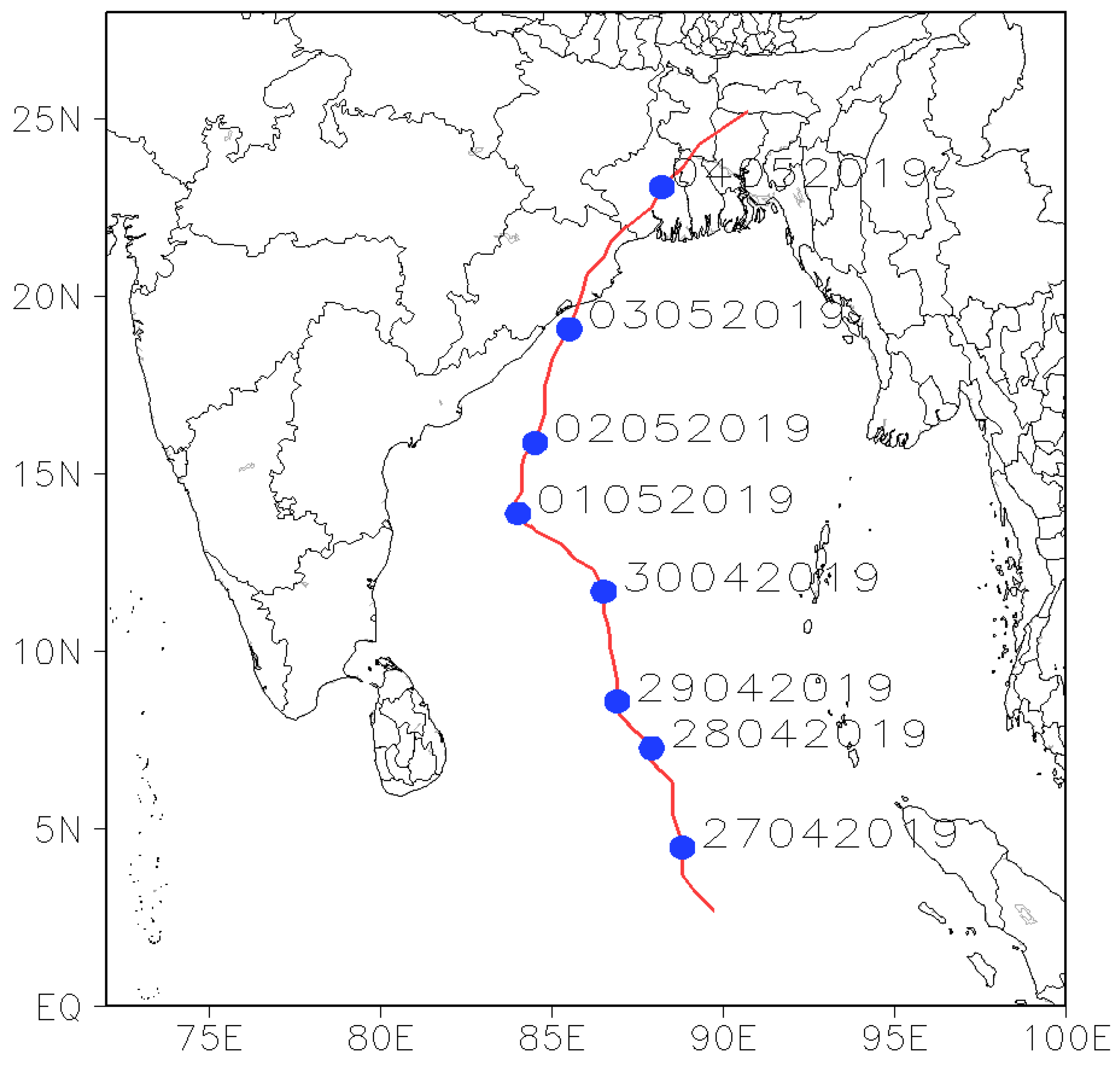
India experiences about two or three tropical cyclones (TCs) each year, with one of them considered severe or more intense [57]. Fani was a severe pre-monsoon storm that originated in the Bay of Bengal region on 26 April 2019 at 0300 UTC, in the depression stage. According to the India Meteorological Department (IMD), the storm slowly moved northward at around 0000 UTC on 27 April and upgraded to a deep depression. It further intensified into a cyclonic storm at 0600 UTC on 27 April and was upgraded to a severe cyclonic storm within the next 6 h. The sea surface temperature around the Fani location was 30–31 °C, which was favorable for further intensification. The central sea level pressure (CSLP) and maximum surface wind (MSW) continued to intensify to about 986 hPa and 28 m/s, respectively, at 1200 UTC on 29 April. In the next 9 h, the storm became a very severe cyclonic storm with an MSW of about 33.5 m/s and reached the stage of Extremely Severe Cyclonic Storm (ESCS) at 1200 UTC on 30 April, with an MSW of about 59.27 m/s and constricted spiral banding covering around the eye. The storm crossed the Odisha coast near Puri between 0230 to 0430 UTC on 3 May 2019. It then continued to move towards West Bengal and weakened over Bangladesh and Central Assam. The observed track of the ESCS from the India Meteorological Department (IMD) is presented in Figure 1. The salient features of Fani are as follows:
- It is considered one of the longest (about 8 days and 9 h) tropical cyclones in the history of the North Indian Ocean [9] and the tenth most severe tropical cyclone in the month of May in the last 52 years [58]. Moreover, it developed near the equator, which is a very rare phenomenon over the North Indian Ocean.
- During landfall, Fani was in the ESCS stage (wind speed was more than 90 knots). It brought heavy rainfall and strong winds to the landfall regions and damaged many infrastructures and properties.
- It caused about 89 fatalities. The projected economic loss was more than 8.1 billion US dollars, and affected areas included the states of Odisha, West Bengal, and Andhra Pradesh in India, as well as East India and Bangladesh.
- Tropical cyclone Fani is considered one of the three worst storms in the past 150 years to make landfall on the Odisha coast causing massive financial losses and social impacts [59].
Figure 1.
Life period of tropical cyclone Fani 2019, observed from IMD best-fit track [The numeric in the figure indicates the date information in the format of DDMMYYYY].
Figure 1.
Life period of tropical cyclone Fani 2019, observed from IMD best-fit track [The numeric in the figure indicates the date information in the format of DDMMYYYY].

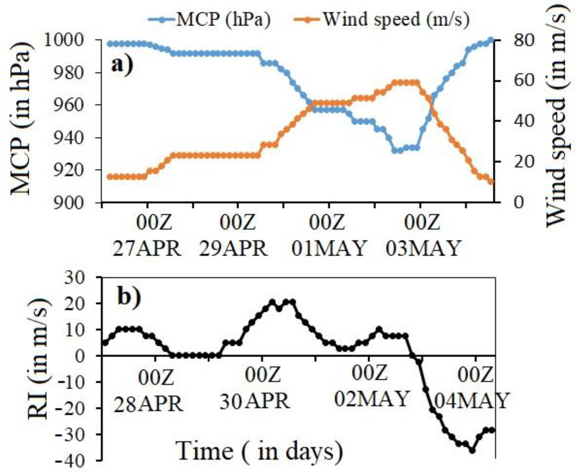
Figure 2.
(a) CSLP and MSW of ESCS Fani 2019 during its life-period and (b) rapid intensification (RI; wind speed more than 15.46 m/s within 24 h) observed from IMD best-fit track.
Figure 2.
(a) CSLP and MSW of ESCS Fani 2019 during its life-period and (b) rapid intensification (RI; wind speed more than 15.46 m/s within 24 h) observed from IMD best-fit track.

2.2. Data and Methodology
In this study, the WRF-ARW version 4.2.2 (hereafter WRF) is utilized, with the vortex following option where inner domains track the TC by following the minimum geopotential height of the 700 hPa pressure surface within the model [60]. This option is recommended for forecasting tropical cyclones, particularly when a well-organized cyclonic vortex is observed over the ocean [61]. A total of 51 vertical levels are used, with the first vertical level at 995 hPa and calculated using the formula (Ph − Pt)/(Ps − Pt), where Ps is 1000 hPa, Pt is 10 hPa, and Ph is the specified height pressure. The physical processes employed in this study include the Kain-Fritsch scheme for cumulus [62], Lin scheme for microphysics [63], Yonsei University scheme for PBL (planetary boundary layer) scheme [64], rapid radiative transfer model (RRTM [65]), and Dudhia’s scheme [66] for shortwave radiation. The cumulus and microphysics schemes are used based on previous studies that reported better forecasts of tropical cyclones over the Bay of Bengal regions with these schemes (e.g., [9,19,20,29]). Table 1 provides details on the model configuration used in the study.
The model was initialized at 0000 UTC on 29 April 2019 and forecasted until 1200 UTC on 3 May 2019. The initial and boundary conditions for model integration were derived from the NCEP-GFS analysis and forecast datasets, respectively, at a resolution of 0.25° × 0.25° (https://rda.ucar.edu/datasets/ds084.1; accessed on 20 February 2020). No external sea surface temperature dataset was used; instead, the same data from the GFS dataset was fed into the model. Time-varying boundary conditions were updated at 6 h intervals. Land use information details were obtained from the United States Geological Survey. Two nested domains were used for simulations, with the outer domain at a 15 km resolution and inner domain at a 3 km resolution. The second domain was used for the moving nest (see Figure 3). Cumulus convection was activated in the outer domain, while it was kept off in the inner domain. Two numerical experiments were conducted using two different air-sea flux parameterization schemes, referred to as FLUX-1 and FLUX-2, respectively, which were specially designed for tropical cyclone forecasts involving alternative Ck (exchange coefficient for temperature and moisture) and Cd (drag coefficient for momentum). The model results were compared with the India Meteorological Department (IMD) best-fit track datasets, satellite observations, and Doppler Weather Radar (DWR) data at Visakhapatnam. The first 6 h of model simulation were considered as model spin-up and were not included in the analysis.
3. Results and Discussions
This section has two parts. In the first part, we compare the results from the two experiments (FLUX-1 and FLUX-2) in terms of the storm’s movement, maximum surface wind speed, minimum central pressure, and landfall with the results obtained from the IMD best-fit track datasets. In the second part, we compare the model’s forecasted results of maximum reflectivity with available Doppler weather radar (DWR) observations from the IMD Visakhapatnam. The relative humidity is compared with ECMWF Reanalysis v5 (ERA5) Global datasets (https://www.ecmwf.int/en/forecasts/dataset/ecmwf-reanalysis-v5; accessed on 20 February 2021). We compare our results with ERA5 reanalysis based on several studies that suggest it provides better wind and other parameters [68,69]. Finally, we compare the water vapor and temperature anomaly with satellite observations [70].
3.1. Forecast of Track and Intensity
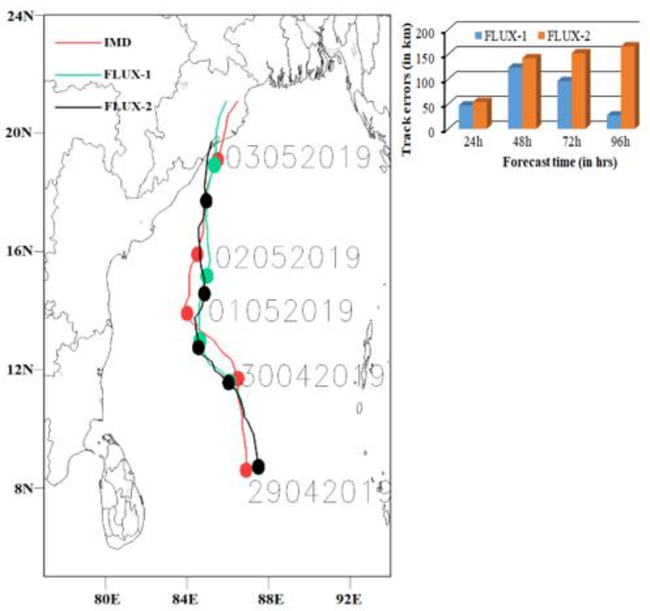
Figure 4 illustrates the model forecasted tracks of tropical cyclone Fani from the FLUX-1 and FLUX-2 experiments, as well as the IMD best-fit track at 3 h intervals, along with their corresponding track errors. The results reveal that the predicted storm track in the FLUX-1 experiment follows the IMD best-fit track data more closely, compared with that in the FLUX-2 experiment. It is observed that the movement of the storm in the FLUX-1 experiment is much closer and faster to the IMD best-fit track than that in the FLUX-2 experiment, which may be due to the translation speed (Figure 5). We notice a relatively closer translation speed of the storm in the FLUX-1 experiment with the IMD observation, suggesting a better movement of the storm in the FLUX-1 experiment than in the FLUX-2 experiment. However, from the second to fourth day, the movement of Fani is slower in the FLUX-2 experiment. The calculated track errors at 24 h, 48 h, 72 h, and 96 h are 47 km, 123 km, 96 km, and 27 km in the FLUX-1 experiment, respectively, while these errors are about 54 km, 142 km, 152 km, and 166 km in the FLUX-2 experiment, respectively (shown as a histogram plot in Figure 4). The mean track error during the entire simulation in the two experiments (FLUX-1 and FLUX-2) is 70 km and 129 km, respectively. Track errors (in km) and translation speed (m/s) at every 3 h interval are also calculated. The results suggest a significant deviation in the tracks after 60 h of forecast, but the track in the FLUX-1 simulation is closer to the observation (Figure 5). The translation speed is calculated using track data on a ±6 h time window [71] and indicates that the movement of the storm in the FLUX-2 experiment is slower compared with that in the FLUX-1 experiment and observation. It is seen that the translation speed is under-predicted in both experiments compared with the observations. The mean translation speeds are about 3.69 m/s and 3.27 m/s in the FLUX-1 and the FLUX-2 experiments, respectively, while this speed is about 3.98 m/s in the IMD observation.
The model simulations show that Fani made landfall near Puri district on 3 May 2019 at 0300 UTC in the FLUX-1 experiment and at 0900 UTC in the FLUX-2 experiment, while observations indicate that it made landfall at 0300 UTC on 3 May 2019. This suggests that the FLUX-1 experiment accurately predicted the landfall time, while the FLUX-2 experiment was delayed by 6 h, indicating slower storm movement in this experiment. The landfall location error was approximately 37 km and 102 km to the left of the observed track in the FLUX-1 and FLUX-2 experiments, respectively, indicating that the FLUX-1 experiment provided better predictions of the storm’s track, movement, landfall time, and location.
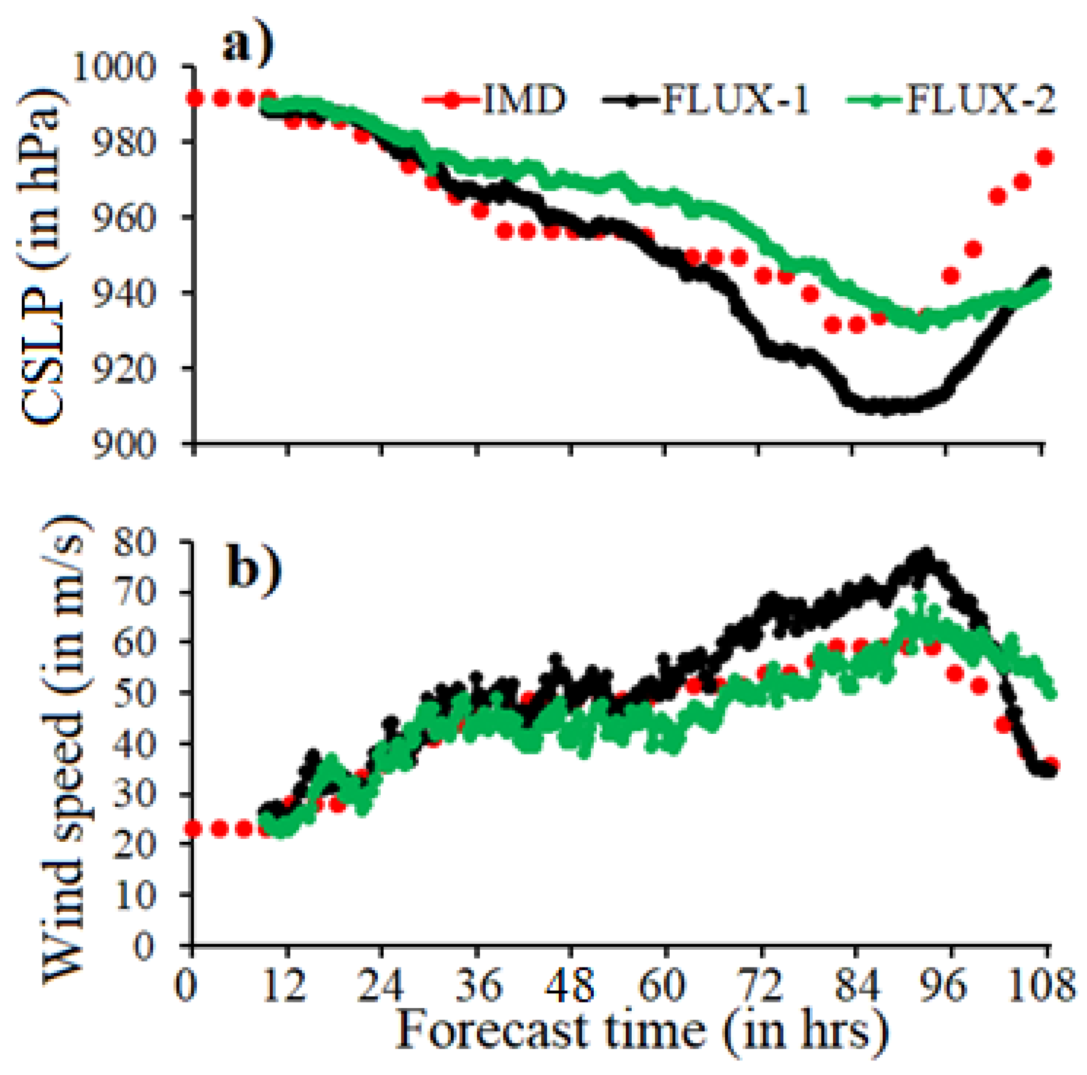
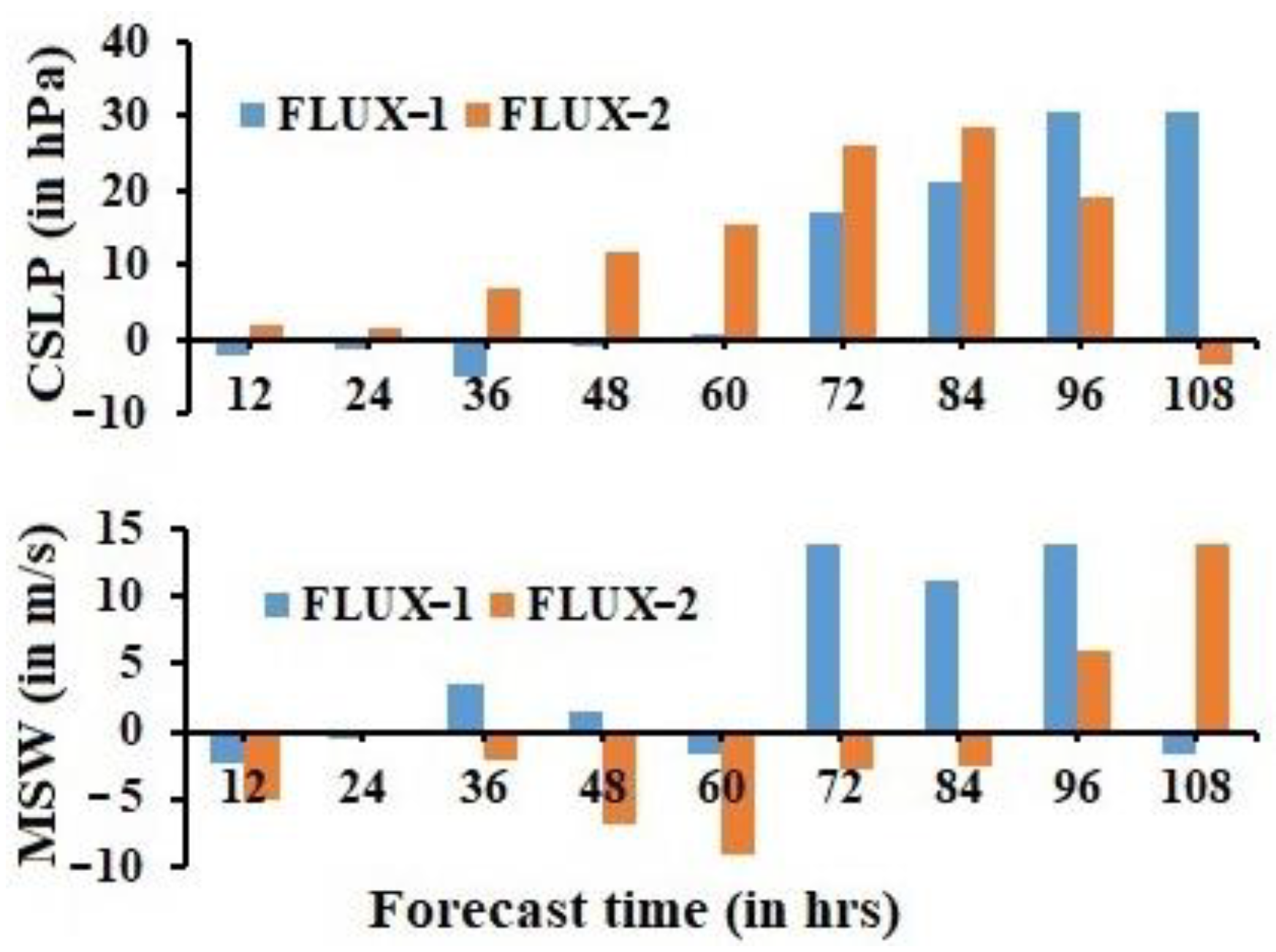
Figure 6 shows the evolution of Fani’s intensity in terms of maximum surface wind speed (MSW) and central sea level pressure (CSLP) calculated from model simulations and the IMD best-fit track. The model data is taken at 15 min intervals, while observations are taken at 3 hourly intervals. The results indicate that the FLUX-1 experiment better reproduced the forecast track, MSW, and CSLP for the first 60 h, while the FLUX-2 experiment performed better for the remaining hours. The FLUX-1 experiment also better captured the intensification and dissipation patterns compared with the FLUX-2 experiment. Figure 7 presents the intensity error (which indicates under-prediction and over-prediction) of CSLP and MSW at 12 h intervals. Results show that the first two days of the forecast were better represented in the FLUX-1 experiment than in the FLUX-2 experiment. The FLUX-1 experiment had an MSW error of less than 2 m/s up to 60 h of the forecast, but the error increased drastically up to 14 m/s in the remaining forecast hours. On the other hand, the 72–96 h forecast of MSW was better in the FLUX-2 experiment. The results suggest that the FLUX-1 experiment overestimated CSLP and MSW during intense stages, indicating a higher simulation error. The experiment also had higher initial errors in MSW and CSLP. Therefore, further research is required to improve the forecast and initial errors by using other physical processes (PBL, microphysics, and cumulus) and data assimilation techniques under the moving nested platform.
3.2. Performance of Model on Forecast of Storm Structure
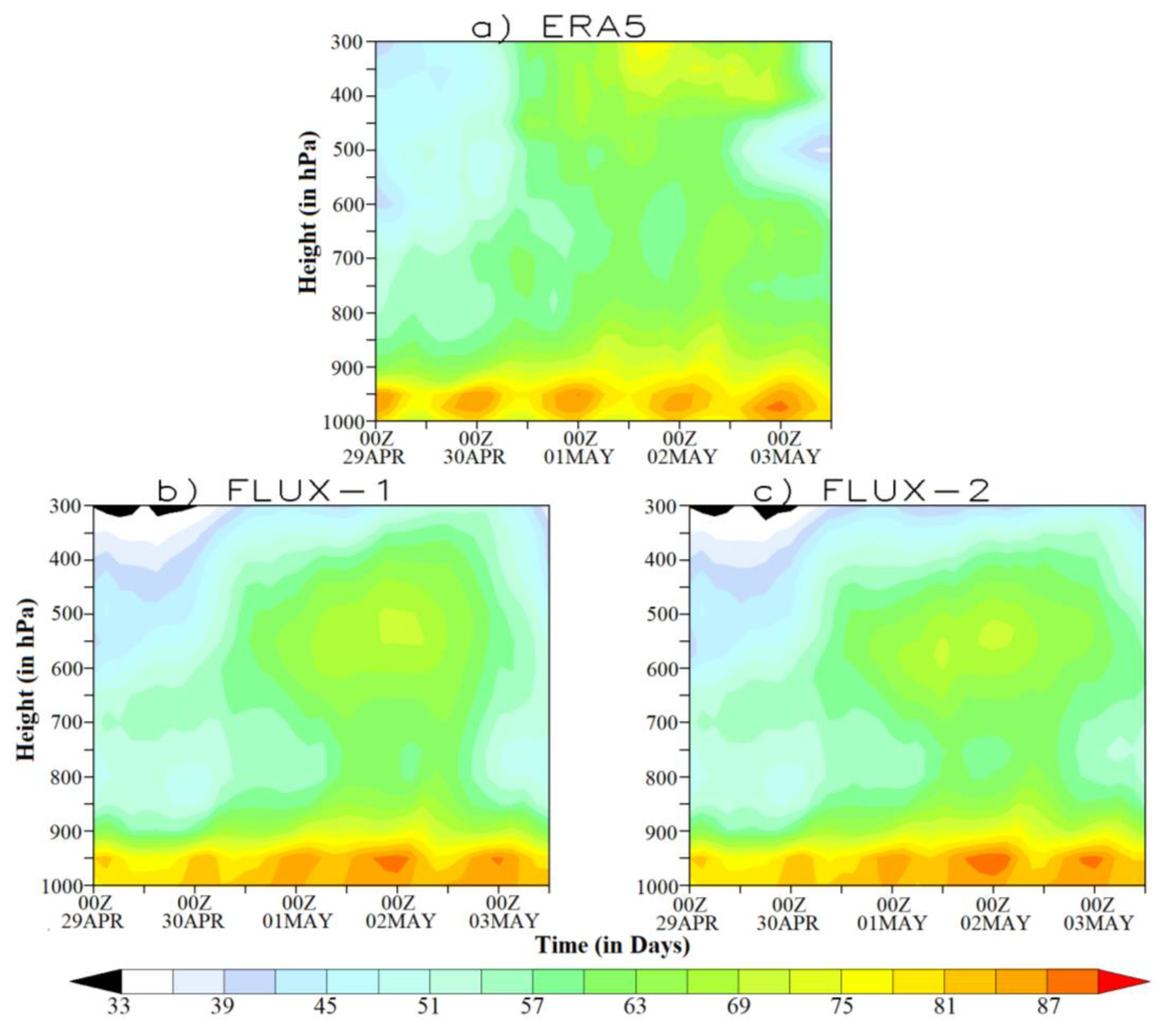
The spatial distribution of the time-height cross-section of relative humidity (in %) is calculated by taking the area average between 81° E to 90° E and 6° N to 23° N in the active region from the model simulations using 15 km horizontal resolution (outer domain) and compared with that from the ERA5 reanalysis datasets with 25 km resolution (Figure 8). The results indicate that the simulated relative humidity from both experiments possess a similar pattern during the entire simulation period with minor differences in magnitude at different heights. The low-level humidity up to 900 hPa in both experiments matches well with that in the ERA5 reanalysis datasets but is slightly higher in magnitude. It is also observed that the simulated middle-level relative humidity between 700 hPa and 500 hPa plays an important role in the intensification of the storm [72,73,74] and is well-correlated with the predicted intensity of the storm. The maximum relative humidity is observed in the simulations from 1200 UTC on 30 April to 1200 UTC on 2 May. A similar pattern of maximum relative humidity is observed in the ERA5 reanalysis during the same time period, but in the lower level between 900 hPa and 600 hPa. We have also analyzed these results by considering a smaller dimension (8° × 8° from the TC center) from the 3 km and 15 km simulations. We find similar qualitative results as in the bigger dimension, but with a slight difference in magnitudes (figures not shown). The high-resolution (3 km) simulation shows comparatively higher values compared with the low-resolution (15 km) simulation. The simulated relative humidity in both cases has a similar pattern during the entire simulation period with minor differences in magnitude at different heights. These results, together with previous studies [72,73,74], suggest that the forecasted maximum intensity of the storm depends on the mid-level relative humidity.
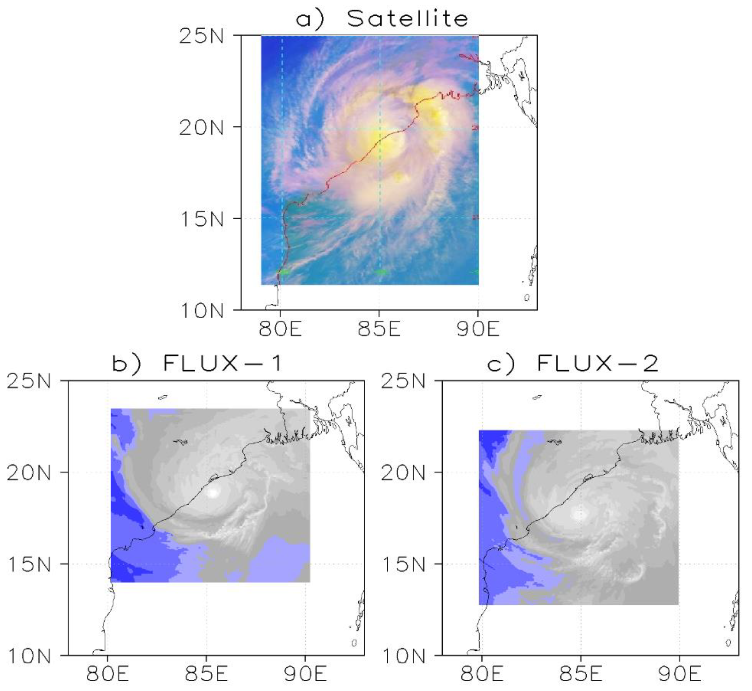
Figure 9 shows the structure of water vapor obtained from the satellite observation at 0000 UTC on 3 May 2019 and the water vapor mixing ratios derived from the model simulations. Here, the structure is presented in terms of the vortex and eye of the storm in the FLUX-1 and FLUX-2 experiments. It is seen that the location of the eye of Fani is slightly better predicted in the FLUX-1 experiment, and this is due to the better forecast of the track in the FLUX-1 experiment compared with that in the FLUX-2 experiment. This indicated that the FLUX-1 experiment provides a better forecast of the structure of Fani over the Bay of Bengal region.
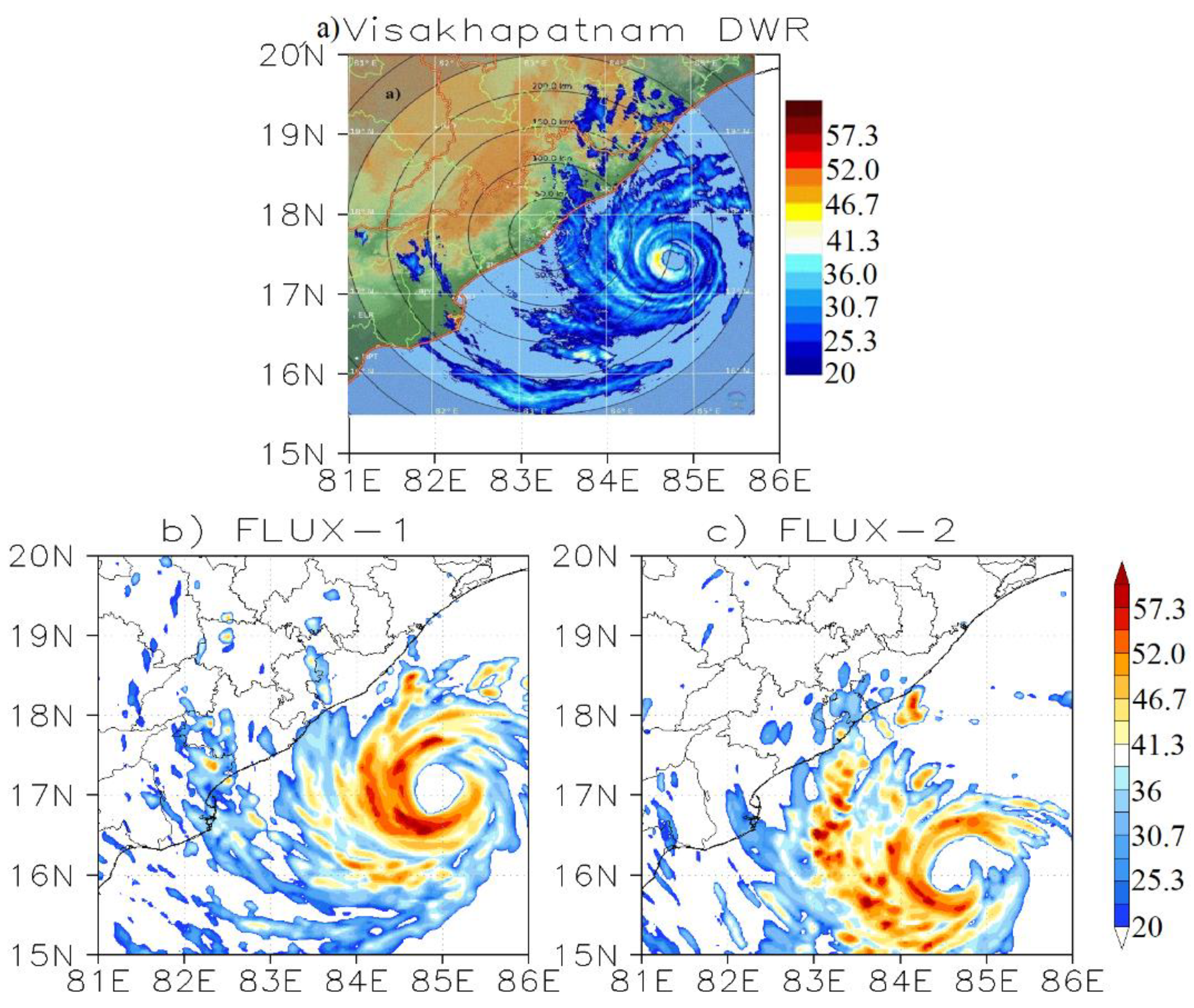
In Figure 10, the maximum reflectivity simulated by the model in both experiments is compared with the Vishakhapatnam Doppler Weather Radar (DWR) at 1130 UTC on 2 May 2019. It can be seen that the spatial distribution of maximum reflectivity of the storm is better predicted in the FLUX-1 experiment compared with the FLUX-2 experiment. However, the magnitude of the reflectivity is over-predicted in both experiments compared with the observation. The maximum reflectivity from the DWR observation is about 46.7 dBZ, whereas in the model it is about 60 dBZ in both experiments. It is also noticed that the pattern of the structure of the storm vortex is better in the FLUX-1 experiment. These results indicate that the performance of the model with the FLUX-1 scheme is quite good towards the prediction of the structure of Fani compared with that of the FLUX-2 scheme, even though the FLUX-1 scheme over-predicted the distribution of reflectivity.
Figure 11 shows the height cross section of temperature anomaly at 03 UTC on 2 May 2019 from model simulations using experiments FLUX-1, FLUX-2, and satellite-derived observations (https://rammb-data.cira.colostate.edu/tc_realtime; accessed on 20 February 2020 [70]). The satellite-derived observation indicates a strong positive temperature anomaly between 9 km and 15 km heights with magnitudes of 2 °C to 6 °C and a larger area at a low-level having cold temperatures. The results from both simulations suggest that the patterns of temperature anomaly are similar in both experiments. A positive anomaly is obtained between 3 km and 17 km heights with a maximum magnitude of about 8 °C and 7 °C in the FLUX-1 and FLUX-2 experiments, respectively. The maximum temperature anomaly in both simulations is noticed at approximately 8.5 km, while in the observation, it is seen about 6 °C at nearly 12 km height. The spatial expansion of the positive anomaly is notably lower in both experiments compared with the observation, but it is slightly better in the FLUX-1 experiment compared with the FLUX-2 experiment.
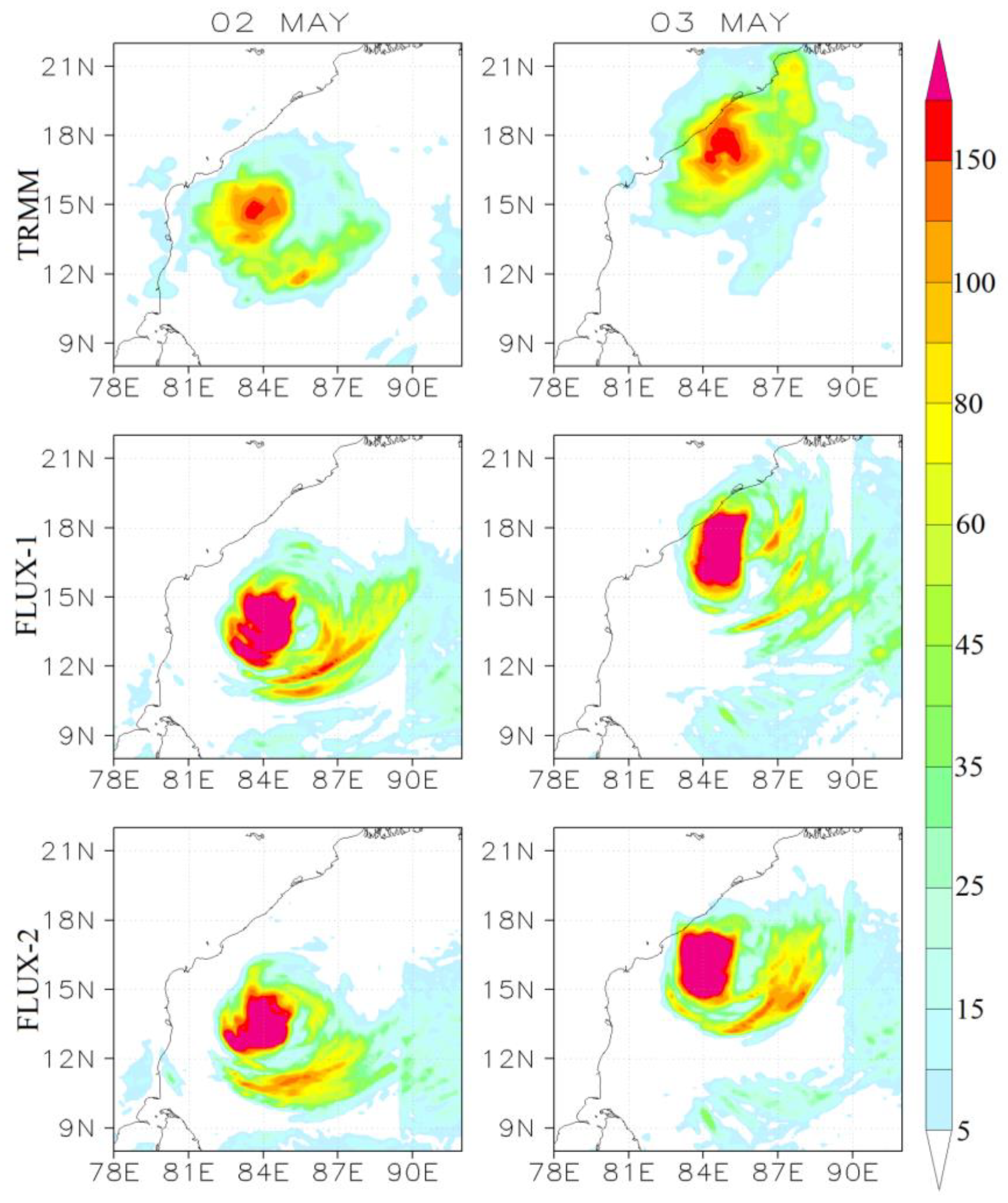
The daily rainfall (24 h accumulated in mm) for 2 May and 3 May 2019 was calculated from model simulations using an outer domain with a resolution of 15 km (Figure 12) and compared with the Tropical Rainfall Measuring Mission (TRMM) daily rainfall data, which has a spatial resolution of about 0.25° × 0.25° (https://disc.gsfc.nasa.gov/datasets/TRMM_3B42_Daily_7; accessed on 25 January 2023). The results show that the forecasted daily rainfalls on both days were over-predicted in the core region of the storm compared with the TRMM observation. The maximum forecasted rainfall in the core region was seen to be more than 250 mm, while it was noticed to be about 200 mm in the TRMM observation. The spatial distribution of the rainfall and the right-side cloud band pattern were well-captured in both experiments for 2 May. However, the model was not able to capture the rainfall over the land region for 3 May in both experiments, although it was slightly better predicted in the FLUX-1 experiment compared with the FLUX-2 experiment.
Overall, the results indicate that the storm movement, intensity, and structure were well-represented in the FLUX-1 experiment. This could be due to the heat and moisture representation [55,56], as the FLUX-1 experiment uses the enthalpy coefficient as [Donelan Cd (drag coefficient for momentum) + constant Z0q for alternative Ck (exchange coefficient for temperature and moisture)], whereas the FLUX-2 experiment uses it as [Donelan Cd + Garratt Ck]. The enthalpy coefficient may have played a major role in reproducing a proper initiation and development of the storm in the FLUX-1 experiment. However, further comparative research is required to confirm this. Therefore, we suggest more research on this issue, specifically focusing on each coefficient’s contribution towards the storm movement, intensity, and structure.
4. Conclusions
The present study evaluates the sensitivity of the air-sea flux parameterization schemes, namely FLUX-1 and FLUX-2, in predicting the tropical cyclone “Fani,” which developed over the Bay of Bengal region in April 2019. The study evaluates the prediction of the storm’s track, intensity, and structure, including relative humidity, temperature anomaly, maximum reflectivity, and water vapor. The major findings of the study are as follows:
- The use of the moving nested domain method in WRF-ARW accurately simulates the track of the storm Fani with both flux parameterization schemes. Comparison between the two schemes indicates that the FLUX-1 experiment better simulates the storm track than the FLUX-2 experiment. Track errors in the FLUX-1 experiment are approximately 47 km, 123 km, 96 km, and 27 km on day 1 to day 4, respectively.
- The FLUX-1 experiment more accurately predicts the time and location of Fani’s landfall, with the landfall time in this experiment matching well with the observation and a landfall location error of approximately 37 km.
- The FLUX-1 experiment provides a better forecast of rapid intensification and dissipation patterns. The forecast of the first 60 hours’ intensity is better represented in the FLUX-1 experiment, while the forecast of remaining hours’ intensity is better represented in the FLUX-2 experiment.
- The structure of Fani, in terms of relative humidity, maximum reflectivity, and temperature anomaly, is well simulated in both experiments.
Overall, the results suggest that the performance of the WRF-ARW model with the FLUX-1 experiment is better suited for predicting tropical cyclone Fani compared with the FLUX-2 experiment. However, these findings are based on only one tropical cyclone simulation, and therefore a more extensive number of cases, including coupled ocean mixed layer depth and time-varying SST, must be studied to make a robust conclusion.
5. Limitation and Future Studies
The investigations presented here are preliminary ideas using the moving nested domain method over the Bay of Bengal region. Similar modeling studies will be conducted in the future with more cases over the North Indian Ocean. Additionally, it is important to test the model’s skill using the moving nested domain method in comparison with the stationary domain method. It is worth mentioning that a single case study is not sufficient to draw any conclusions. Therefore, a comprehensive study with a larger number of cases in both the pre- and post-monsoon seasons is suggested for a more robust conclusion.
Author Contributions
Conceptualization—K.S.S.; methodology—K.S.S.; software—K.S.S.; validation—K.S.S., S.M., S.N. and H.P.N.; formal analysis—K.S.S.; investigation—K.S.S., S.M., S.N. and H.P.N.; data curation—K.S.S.; writing—original draft preparation—K.S.S.; writing—review and editing—K.S.S., S.M., S.N., H.P.N. and S.D.; visualization—K.S.S., H.P.N., S.M., S.N. and S.D.; supervision—K.S.S. All authors have read and agreed to the published version of the manuscript.
Funding
The author sincerely acknowledges the financial support of the DST-SERB (Project file no. ECR/2018/001185) and VIT SEED Grant File No.: SG20210089.
Institutional Review Board Statement
Not applicable.
Informed Consent Statement
Not applicable.
Data Availability Statement
The India Meteorological Department best-fit track data and CIRA https://rammb-data.cira.colostate.edu/tc_realtime; accessed on 20 February 2020, data were used for validation and are freely available.
Acknowledgments
The author sincerely acknowledges the financial support of the DST-SERB (Project file no. ECR/2018/001185) and VIT SEED Grant File No.: SG20210089; the IMD and CIRA for providing the cyclone best-fit track datasets and satellite observations, respectively; and NCEP and NCAR for providing GFS analysis and forecast datasets, and the WRF modeling system.
Conflicts of Interest
The authors declare no conflict of interest.
References
- Webster, P.J.; Holland, G.J.; Curry, J.A.; Chang, H.R. Changes in tropical cyclone number, duration, and intensity in a warming environment. Science 2005, 309, 1844–1846. [Google Scholar] [CrossRef] [PubMed] [Green Version]
- Balaji, M.; Chakraborty, A.; Mandal, M. Changes in tropical cyclone activity in North Indian Ocean during satellite era (1981–2014). Int. J. Climatol. 2018, 38, 2819–2837. [Google Scholar] [CrossRef]
- Albert, J.; Krishnan, A.; Bhaskaran, P.K.; Singh, K.S. Role and influence of key atmospheric parameters in large-scale environmental flow associated with tropical cyclogenesis and ENSO in the North Indian Ocean basin. Clim. Dyn. 2021, 58, 17–34. [Google Scholar] [CrossRef]
- Nayak, S.; Takemi, T. Robust responses of typhoon hazards in northern Japan to global warming climate: Cases of landfalling typhoons in 2016. Meteorol. Appl. 2020, 27, e1954. [Google Scholar] [CrossRef]
- Nayak, S.; Takemi, T. Typhoon induced precipitation characterization over northern Japan: A case study for typhoons in 2016. Prog. Earth Planet. Sci. 2020, 7, 39. [Google Scholar] [CrossRef]
- Morimoto, J.; Aiba, M.; Furukawa, F.; Mishima, Y.; Yoshimura, N.; Nayak, S.; Takemi, T.; Haga, C.; Matsui, T.; Nakamura, F. Risk assessment of forest disturbance by typhoons with heavy precipitation in northern Japan. For. Ecol. Manag. 2021, 479, 118521. [Google Scholar] [CrossRef]
- Nayak, S.; Takemi, T. Dynamical downscaling of Typhoon Lionrock (2016) for assessing the resulting hazards under global warming. J. Meteorol. Soc. Jpn. 2019, 97, 69–88. [Google Scholar] [CrossRef] [Green Version]
- Nayak, S.; Takemi, T. Quantitative estimations of hazards resulting from Typhoon Chanthu (2016) for assessing the impact in current and future climate. Hydrol. Res. Lett. 2019, 13, 20–27. [Google Scholar] [CrossRef] [Green Version]
- Singh, K.S.; Albert, J.; Bhaskaran, P.K.; Alam, P. Assessment of extremely severe cyclonic storms over Bay of Bengal and performance evaluation of ARW model in the prediction of track and intensity. Theor. Appl. Climatol. 2021, 143, 1181–1194. [Google Scholar] [CrossRef]
- Prasad, K.; Rao, Y.R. Simulation Studies on Cyclone Track Prediction by Quasi-Lagrangian Model (QLM) in Some Historical and Recent Cases in the Bay of Bengal, Using Global Re-Analysis and Forecast Grid Point Data Sets; SAARC Meteorological Research Centre: Dhaka, Bangladesh, 2006. [Google Scholar]
- Sudha Rani, N.N.V.; Satyanarayana, A.N.V.; Bhaskaran, P.K. Coastal vulnerability assessment studies over India: A review. Nat. Hazards 2015, 77, 405–428. [Google Scholar] [CrossRef]
- Sahoo, B.; Bhaskaran, P.K. Assessment on historical cyclone tracks in the Bay of Bengal, east coast of India. Int. J. Climatol. 2016, 36, 95–109. [Google Scholar] [CrossRef]
- Albert, J.; Bhaskaran, P.K. Ocean heat content and its role in tropical cyclogenesis for the Bay of Bengal basin. Clim. Dyn. 2020, 55, 3343–3362. [Google Scholar] [CrossRef]
- Mohandas, S.; Ashrit, R. Sensitivity of different convective parameterization schemes on tropical cyclone prediction using a mesoscale model. Nat. Hazards 2014, 73, 213–235. [Google Scholar] [CrossRef]
- Srinivas, C.V.; Bhaskar Rao, D.; Yesubabu, V.; Baskaran, R.; Venkatraman, B. Tropical cyclone predictions over the Bay of Bengal using the high-resolution Advanced Research Weather Research and Forecasting (ARW) model. Q. J. R. Meteorol. Soc. 2013, 139, 1810–1825. [Google Scholar] [CrossRef]
- Steptoe, H.; Savage, N.H.; Sadri, S.; Salmon, K.; Maalick, Z.; Webster, S. Tropical cyclone simulations over Bangladesh at convection permitting 4.4 km & 1.5 km resolution. Sci. Data 2021, 8, 62. [Google Scholar]
- Deshpande, M.; Pattnaik, S.; Salvekar, P.S. Impact of physical parameterization schemes on numerical simulation of super cyclone Gonu. Nat. Hazards 2010, 55, 211–231. [Google Scholar] [CrossRef]
- Osuri, K.K.; Mohanty, U.C.; Routray, A.; Kulkarni, M.A.; Mohapatra, M. Customization of WRF-ARW model with physical parameterization schemes for the simulation of tropical cyclones over North Indian Ocean. Nat. Hazards 2012, 63, 1337–1359. [Google Scholar] [CrossRef]
- Singh, K.S.; Mandal, M. Sensitivity of mesoscale simulation of Aila Cyclone to the parameterization of physical processes using WRF Model. In Monitoring and Prediction of Tropical Cyclones in the Indian Ocean and Climate Change; Springer: Dordrecht, The Netherlands, 2014; pp. 300–308. [Google Scholar]
- Singh, K.S.; Bhaskaran, P.K. Impact of PBL and convection parameterization schemes for prediction of severe land-falling Bay of Bengal cyclones using WRF-ARW model. J. Atmos. Sol.-Terr. Phys. 2017, 165, 10–24. [Google Scholar] [CrossRef]
- Vinodkumar; Chandrasekhar, A.; Alapaty, K.; Niyogi, D. The impacts of indirect soil moisture assimilation and direct surface temperature and humidity assimilation on a mesoscale model simulation of an Indian monsoon depression. J. Appl. Meteorol. Climatol. 2008, 47, 1393–1412. [Google Scholar] [CrossRef]
- Srinivas, C.V.; Yesubabu, V.; Venkatesan, R.; Ramakrishna, S.S. Impact of assimilation of conventional and satellite meteorological observations on the numerical simulation of a Bay of Bengal tropical cyclone of November 2008 near Tamilnadu using WRF model. Meteorol. Atmos. Phys. 2010, 110, 19–44. [Google Scholar] [CrossRef]
- Rakesh, V.; Singh, R.; Pal, P.K.; Joshi, P.C. Impacts of satellite observed winds and total precipitable water on WRF short-range forecasts over the Indian region during the 2006 summer monsoon. Weather Forecast. 2009, 24, 1706–1731. [Google Scholar] [CrossRef]
- Rakesh, V.; Singh, R.; Pal, P.K.; Joshi, P.C. Impact of satellite soundings on the simulation of heavy rainfall associated with tropical depressions. Nat. Hazards 2011, 58, 945–980. [Google Scholar] [CrossRef]
- Osuri, K.K.; Mohanty, U.C.; Routray, A.; Mohapatra, M. The impact of satellite-derived wind data assimilation on track, intensity and structure of tropical cyclones over the North Indian Ocean. Int. J. Remote Sens. 2012, 33, 1627–1652. [Google Scholar] [CrossRef]
- Routray, A.; Mohanty, U.C.; Osuri, K.K.; Kar, S.C.; Niyogi, D. Impact of satellite radiance data on simulations of Bay of Bengal tropical cyclones using the WRF-3DVAR modeling system. IEEE Trans. Geosci. Remote Sens. 2016, 54, 2285–2303. [Google Scholar] [CrossRef]
- Osuri, K.K.; Nadimpalli, R.; Mohanty, U.C.; Niyogi, D. Prediction of rapid intensification of tropical cyclone Phailin over the Bay of Bengal using the HWRF modelling system. Q. J. R. Meteorol. Soc. 2017, 143, 678–690. [Google Scholar] [CrossRef]
- Singh, K.S.; Bhaskaran, P.K. Impact of lateral boundary and initial conditions in the prediction of Bay of Bengal cyclones using WRF model and its 3D-VAR data assimilation system. J. Atmos. Sol.-Terr. Phys. 2018, 175, 64–75. [Google Scholar] [CrossRef]
- Singh, K.S.; Bhaskaran, P.K. Prediction of land-falling Bay of Bengal cyclones during 2013 using the high resolution Weather Research and Forecasting model. Meteorol. Appl. 2020, 27, e1850. [Google Scholar] [CrossRef] [Green Version]
- Nadimpalli, R.; Srivastava, A.; Prasad, V.S.; Osuri, K.K.; Das, A.K.; Mohanty, U.C.; Niyogi, D. Impact of INSAT-3D/3DR radiance data assimilation in predicting tropical cyclone Titli over the Bay of Bengal. IEEE Trans. Geosci. Remote Sens. 2020, 58, 6945–6957. [Google Scholar] [CrossRef]
- Singh, K.S.; Tyagi, B. Impact of data assimilation and air-sea flux parameterization schemes on the prediction of cyclone Phailin over the Bay of Bengal using the WRF-ARW model. Meteorol. Appl. 2019, 26, 36–48. [Google Scholar] [CrossRef] [Green Version]
- Singh, K.S.; Mandal, M.; Bhaskaran, P.K. Impact of radiance data assimilation on the prediction performance of cyclonic storm SIDR using WRF-3DVAR modelling system. Meteorol. Atmos. Phys. 2019, 131, 11–28. [Google Scholar] [CrossRef]
- Lok, C.C.; Chan, J.C.; Toumi, R. Importance of Air-Sea Coupling in Simulating Tropical Cyclone Intensity at Landfall. Adv. Atmos. Sci. 2022, 39, 1777–1786. [Google Scholar] [CrossRef]
- Ricchi, A.; Bonaldo, D.; Cioni, G.; Carniel, S.; Miglietta, M.M. Simulation of a flash-flood event over the Adriatic Sea with a high-resolution atmosphere-ocean-wave coupled system. Sci. Rep. 2021, 11, 9388. [Google Scholar] [CrossRef]
- Warner, J.C.; Armstrong, B.; He, R.; Zambon, J.B. Development of a coupled ocean-atmosphere-wave-sediment transport (COAWST) modeling system. Ocean. Model. 2010, 35, 230–244. [Google Scholar] [CrossRef] [Green Version]
- Andreas, E.L. The Impact of Sea Spray on Air-Sea Fluxes in Coupled Atmosphere-Ocean Models; Regions Research and Engineering Laboratory: Hanover, NH, USA, 2002. [Google Scholar]
- Chelton, D.B.; Esbensen, S.K.; Schlax, M.G.; Thum, N.; Freilich, M.H.; Wentz, F.J.; Gentemann, C.L.; McPhaden, M.J.; Schopf, P.S. Observations of coupling between surface wind stress and sea surface temperature in the eastern tropical Pacific. J. Clim. 2001, 14, 1479–1498. [Google Scholar] [CrossRef]
- O’Neill, L.W.; Esbensen, S.K.; Thum, N.; Samelson, R.M.; Chelton, D.B. Dynamical analysis of the boundary layer and surface wind responses to mesoscale SST perturbations. J. Clim. 2010, 23, 559–581. [Google Scholar] [CrossRef] [Green Version]
- Crnivec, N.; Smith, R.K.; Kilroy, G. Dependence of tropical cyclone intensification rate on sea-surface temperature. Q. J. R. Meteorol. Soc. 2016, 142, 1618–1627. [Google Scholar] [CrossRef]
- Kanada, S.; Tsujino, S.; Aiki, H.; Yoshioka, M.K.; Miyazawa, Y.; Tsuboki, K.; Takayabu, I. Impacts of SST patterns on rapid intensification of Typhoon Megi (2010). J. Geophys. Res. Atmos. 2017, 122, 13–245. [Google Scholar] [CrossRef] [Green Version]
- Meroni, A.N.; Parodi, A.; Pasquero, C. Role of SST patterns on surface wind modulation of a heavy midlatitude precipitation event. J. Geophys. Res. Atmos. 2018, 123, 9081–9096. [Google Scholar] [CrossRef]
- Gopalakrishnan, S.G.; Surgi, N.; Tuleya, R.; Janjic, Z. NCEP’s two-way-interactive-moving-nest NMM-WRF modeling system for hurricane forecasting. In Proceedings of the 27th Conference on Hurricanes and Tropical Meteorology, Monterey, CA, USA, 23–24 April 2006. [Google Scholar]
- Wu, Z.; Zhang, Y.; Xie, Y.; Zhang, L.; Zheng, H. Radiance-based assessment of bulk microphysics models with seven hydrometeor species in forecasting Super-typhoon Lekima (2019) near landfall. Atmos. Res. 2022, 273, 106173. [Google Scholar] [CrossRef]
- Wu, Z.; Zhang, Y.; Zhang, L.; Zheng, H. Improving the WRF Forecast of Landfalling Tropical Cyclones over the Asia-Pacific Region by Constraining the Cloud Microphysics Model with GPM Observations. Geophys. Res. Lett. 2022, 49, e2022GL100053. [Google Scholar] [CrossRef]
- Liao, X.; Li, T.; Ma, C. Moist Static Energy and Secondary Circulation Evolution Characteristics during the Rapid Intensification of Super Typhoon Yutu (2007). Atmosphere 2022, 13, 1105. [Google Scholar] [CrossRef]
- Chen, X.; Xue, M.; Fang, J. Rapid intensification of Typhoon Mujigae (2015) under different sea surface temperatures: Structural changes leading to rapid intensification. J. Atmos. Sci. 2018, 75, 4313–4335. [Google Scholar] [CrossRef]
- Ye, L.; Li, Y.; Gao, Z. Evaluation of Air–Sea Flux Parameterization for Typhoon Mangkhut Simulation during Intensification Period. Atmosphere 2022, 13, 2133. [Google Scholar] [CrossRef]
- Sanders, F.; Gyakum, J.R. Synoptic-dynamic climatology of the “bomb”. Mon. Weather. Rev. 1980, 108, 1589–1606. [Google Scholar] [CrossRef]
- Zhang, L.; Zhang, X.; Chu, P.C.; Guan, C.; Fu, H.; Chao, G.; Han, G.; Li, W. Impact of sea spray on the Yellow and East China Seas thermal structure during the passage of Typhoon Rammasun (2002). J. Geophys. Res. Ocean. 2017, 122, 7783–7802. [Google Scholar] [CrossRef]
- Andreas, E.L.; Persson, P.O.G.; Hare, J.E. A bulk turbulent air–sea flux algorithm for high-wind, spray conditions. J. Phys. Oceanogr. 2008, 38, 1581–1596. [Google Scholar] [CrossRef]
- Black, P.G.; D’Asaro, E.A.; Drennan, W.M.; French, J.R.; Niiler, P.P.; Sanford, T.B.; Terrill, E.J.; Walsh, E.J.; Zhang, J.A. Air–sea exchange in hurricanes: Synthesis of observations from the coupled boundary layer air–sea transfer experiment. Bull. Am. Meteorol. Soc. 2007, 88, 357–374. [Google Scholar] [CrossRef] [Green Version]
- Donelan, M.A.; Drennan, W.M.; Katsaros, K.B. The air–sea momentum flux in conditions of Wind Sea and swell. J. Phys. Oceanogr. 1997, 27, 2087–2099. [Google Scholar] [CrossRef]
- Fairall, C.W.; Banner, M.L.; Peirson, W.L.; Asher, W.; Morison, R.P. Investigation of the physical scaling of sea spray spume droplet production. J. Geophys. Res. Ocean. 2009, 114, C10001, 1–19. [Google Scholar] [CrossRef]
- Obermann, A.; Edelmann, B.; Ahrens, B. Influence of sea surface roughness length parameterization on Mistral and Tramontane simulations. Adv. Sci. Res. 2016, 13, 107–112. [Google Scholar] [CrossRef] [Green Version]
- Kueh, M.T.; Chen, W.M.; Sheng, Y.F.; Lin, S.C.; Wu, T.R.; Yen, E.; Tsai, Y.L.; Lin, C.Y. Effects of horizontal resolution and air–sea flux parameterization on the intensity and structure of simulated Typhoon Haiyan (2013). Nat. Hazards Earth Syst. Sci. 2019, 19, 1509–1539. [Google Scholar] [CrossRef] [Green Version]
- Powell, M.D.; Vickery, P.J.; Reinhold, T.A. Reduced drag coefficient for high wind speeds in tropical cyclones. Nature 2003, 422, 279–283. [Google Scholar] [CrossRef]
- Deshpande, M.; Singh, V.K.; Ganadhi, M.K.; Roxy, M.K.; Emmanuel, R.; Kumar, U. Changing status of tropical cyclones over the north Indian Ocean. Clim. Dyn. 2021, 57, 3545–3567. [Google Scholar] [CrossRef]
- Kumar, S.; Lal, P.; Kumar, A. Turbulence of tropical cyclone 'Fani' in the Bay of Bengal and Indian subcontinent. Nat. Hazards 2020, 103, 1613–1622. [Google Scholar] [CrossRef]
- Chatterjee, S. Analytical Study of North Indian Oceanic Cyclonic Disturbances with Special Reference to Extremely Severe Cyclonic Storm Fani: Meteorological Variability, India’s Preparedness with Terrible Aftermath. Nat. Hazards Earth Syst. Sci. Discuss. 2020, 1–24. [Google Scholar]
- Nolan, D.S.; McNoldy, B.D.; Yunge, J. Evaluation of the surface wind field over land in WRF simulations of Hurricane Wilma (2005). Part I: Model initialization and simulation validation. Mon. Weather. Rev. 2021, 149, 679–695. [Google Scholar] [CrossRef]
- Skamarock, W.C.; Klemp, J.B.; Dudhia, J.; Gill, D.O.; Barker, D.M.; Duda, M.G.; Huang, X.Y.; Wang, W.; Powers, J.G. A Description of the Advanced Research WRF; National Center for Atmospheric Research: Boulder, CO, USA, 2008; Version 3. [Google Scholar]
- Kain, J.S. The Kain–Fritsch convective parameterization: An update. J. Appl. Meteorol. 2004, 43, 170–181. [Google Scholar] [CrossRef]
- Lin, Y.L.; Farley, R.D.; Orville, H.D. Bulk parameterization of the snow field in a cloud model. J. Appl. Meteorol. Climatol. 1983, 22, 1065–1092. [Google Scholar] [CrossRef]
- Hong, S.Y.; Noh, Y.; Dudhia, J. A new vertical diffusion package with an explicit treatment of entrainment processes. Mon. Weather. Rev. 2006, 134, 2318–2341. [Google Scholar] [CrossRef] [Green Version]
- Mlawer, E.J.; Taubman, S.J.; Brown, P.D.; Iacono, M.J.; Clough, S.A. Radiative transfer for inhomogeneous atmospheres: RRTM, a validated correlated-k model for the longwave. J. Geophys. Res. Atmos. 1997, 102, 16663–16682. [Google Scholar] [CrossRef] [Green Version]
- Dudhia, J. Numerical study of convection observed during the winter monsoon experiment using a mesoscale two-dimensional model. J. Atmos. Sci. 1989, 46, 3077–3107. [Google Scholar] [CrossRef]
- Niu, G.Y.; Yang, Z.L.; Mitchell, K.E.; Chen, F.; Ek, M.B.; Barlage, M.; Kumar, A.; Manning, K.; Niyogi, D.; Rosero, E.; et al. The community Noah land surface model with multi parameterization options (Noah-MP): 1. Model description and evaluation with local-scale measurements. J. Geophys. Res. Atmos. 2011, 116, D12109. [Google Scholar] [CrossRef] [Green Version]
- Rennie, M.P.; Isaksen, L.; Weiler, F.; de Kloe, J.; Kanitz, T.; Reitebuch, O. The impact of Aeolus wind retrievals on ECMWF global weather forecasts. Q. J. R. Meteorol. Soc. 2021, 147, 3555–3586. [Google Scholar] [CrossRef]
- Carvalho, D.; Rocha, A.; Gómez-Gesteira, M.; Santos, C.S. WRF wind simulation and wind energy production estimates forced by different reanalyses: Comparison with observed data for Portugal. Appl. Energy 2014, 117, 116–126. [Google Scholar] [CrossRef]
- Demuth, J.L.; De Maria, M.; Knaff, J.A.; Vonder Haar, T.H. Evaluation of Advanced Microwave Sounding Unit tropical-cyclone intensity and size estimation algorithms. J. Appl. Meteorol. 2004, 43, 282–296. [Google Scholar] [CrossRef]
- Mei, W.; Pasquero, C.; Primeau, F. The effect of translation speed upon the intensity of tropical cyclones over the tropical ocean. Geophys. Res. Lett. 2012, 39, L07801, 1–6. [Google Scholar] [CrossRef] [Green Version]
- Kaplan, J.; De Maria, M.; Knaff, J.A. A revised tropical cyclone rapid intensification index for the Atlantic and eastern North Pacific basins. Weather Forecast. 2010, 25, 220–241. [Google Scholar] [CrossRef]
- Shu, S.; Ming, J.; Chi, P. Large-scale characteristics and probability of rapidly intensifying tropical cyclones in the western North Pacific basin. Weather Forecast. 2012, 27, 411–423. [Google Scholar] [CrossRef]
- Wang, Y.; Rao, Y.; Tan, Z.M.; Schönemann, D. A statistical analysis of the effects of vertical wind shear on tropical cyclone intensity change over the western North Pacific. Mon. Weather. Rev. 2015, 143, 3434–3453. [Google Scholar] [CrossRef]
Figure 3.
Double nested model domains (15 km and 3 km) with inner domain are taken as the moving nest; the shaded region shows the wind field (in m/s) during initialization at 0000 UTC on 29 April 2019.
Figure 3.
Double nested model domains (15 km and 3 km) with inner domain are taken as the moving nest; the shaded region shows the wind field (in m/s) during initialization at 0000 UTC on 29 April 2019.

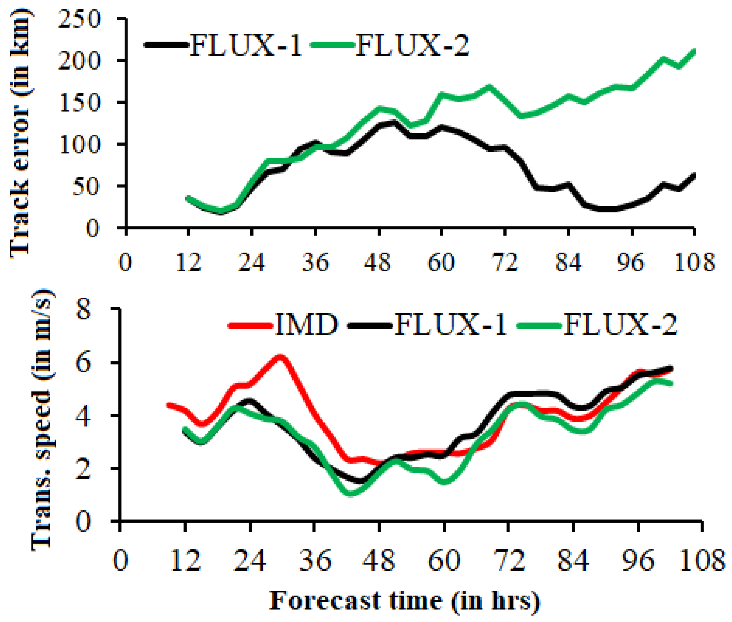
Figure 4.
Model simulated tracks from the FLUX-1 and FLUX-2 experiments along with IMD best-fit track at every 3 h interval (date is considered from IMD best fit-track), and track errors (in km) of both the experiments (The numeric in the figure indicates the date information in DDMMYYYY).
Figure 4.
Model simulated tracks from the FLUX-1 and FLUX-2 experiments along with IMD best-fit track at every 3 h interval (date is considered from IMD best fit-track), and track errors (in km) of both the experiments (The numeric in the figure indicates the date information in DDMMYYYY).

Figure 5.
Model simulated track errors (in km) and translation speed (m/s) from simulations along with IMD best-fit track at every 3 h interval.
Figure 5.
Model simulated track errors (in km) and translation speed (m/s) from simulations along with IMD best-fit track at every 3 h interval.

Figure 6.
Model simulated intensity from the FLUX-1 and FLUX-2 experiments in terms of (a) CSLP (in hPa) and (b) wind speed (in m/s) along with IMD best-fit track dataset.
Figure 6.
Model simulated intensity from the FLUX-1 and FLUX-2 experiments in terms of (a) CSLP (in hPa) and (b) wind speed (in m/s) along with IMD best-fit track dataset.

Figure 7.
Simulated intensity errors from the FLUX-1 and FLUX-2 experiments in terms of CSLP (in hPa) and MSW (in m/s).
Figure 7.
Simulated intensity errors from the FLUX-1 and FLUX-2 experiments in terms of CSLP (in hPa) and MSW (in m/s).

Figure 8.
Area averaged relative humidity (in %) in the active region (longitude from 81° E to 90° E and latitude from 6° N to 23° N) obtained from (a) the ERA5 reanalysis datasets and (b,c) simulations.
Figure 8.
Area averaged relative humidity (in %) in the active region (longitude from 81° E to 90° E and latitude from 6° N to 23° N) obtained from (a) the ERA5 reanalysis datasets and (b,c) simulations.

Figure 9.
Structure of water vapor content at 0000 UTC on 3 May 2019 obtained from (a) the Satellite observation, (b) the FLUX-1 experiment, and (c) the FLUX-2 experiment. Figure 9a was adopted from the Regional and Mesoscale Meteorology Branch (https://rammb-data.cira.colostate.edu/tc_realtime/storm.asp?storm_identifier=io012019; accessed on 20 February 2020). This figure is used to see the structures only to visualize if the structure is correctly reduced in the model simulation.

Figure 10.
Maximum reflectivity (in dBZ; x-axis shows longitude and y-axis shows latitude) at 1130 UTC on 2 May 2019 obtained from (a) Visakhapatnam DWR, (b) the FLUX-1, and (c) the FLUX-2 experiment.
Figure 10.
Maximum reflectivity (in dBZ; x-axis shows longitude and y-axis shows latitude) at 1130 UTC on 2 May 2019 obtained from (a) Visakhapatnam DWR, (b) the FLUX-1, and (c) the FLUX-2 experiment.

Figure 11.
Temperature anomaly at 03 UTC on 2 May 2019 obtained from (a) the satellite observation, (b) the FLUX-1 experiment, and (c) the FLUX-2 experiment (considered from the center of the tropical cyclone to 600 km varying from west to east).
Figure 11.
Temperature anomaly at 03 UTC on 2 May 2019 obtained from (a) the satellite observation, (b) the FLUX-1 experiment, and (c) the FLUX-2 experiment (considered from the center of the tropical cyclone to 600 km varying from west to east).

Figure 12.
Daily rainfall (in mm) on 2 May and 3 May 2019 from TRMM and model forecast.


Table 1.
WRF Model configuration used in the study.
| Dynamical Core | Non-Hydrostatic, WRF-ARW (Version 4.2) |
|---|---|
| Initial condition | GFS analysis (0.25° × 0.25°) |
| Model resolution | 15 km × 15 km (D1; fixed domain) and 3 km × 3 km (D2; moving nested domain) |
| Model time steps | 75 s (D1) and 15 s (D2) |
| Vertical levels | 51 (first vertical level at 995 hPa with high resolution in the boundary layer) |
| Cumulus parameterization | KF (used for outer domain only) [62] |
| Microphysics | Lin [63] |
| PBL scheme | YSU scheme [64] |
| Short and long wave radiation | RRTM [65], Dudhia [66] |
| Surface layer | Noah Land Surface model [67] |
| Enthalpy coefficient | FLUX-1: experiment (Donelan Cd (drag coefficient for momentum) + constant Z0q for alternative Ck (exchange coefficient for temp and moisture)) FLUX-2: experiment (Donelan Cd + Garratt Ck) Garratt formulation, slightly different forms for heat and moisture. |
| Number of grid points | 232 × 265 (D1) and 326 × 321 (D2) |
| Forecast length and initialization | 4 days 12 h, 0000 UTC of 29 April 2019 |
| Vortex interval | 15 min |
| Track level | 850 hPa |
Disclaimer/Publisher’s Note: The statements, opinions and data contained in all publications are solely those of the individual author(s) and contributor(s) and not of MDPI and/or the editor(s). MDPI and/or the editor(s) disclaim responsibility for any injury to people or property resulting from any ideas, methods, instructions or products referred to in the content. |
© 2023 by the authors. Licensee MDPI, Basel, Switzerland. This article is an open access article distributed under the terms and conditions of the Creative Commons Attribution (CC BY) license (https://creativecommons.org/licenses/by/4.0/).
Share and Cite
MDPI and ACS Style
Singh, K.S.; Nayak, S.; Maity, S.; Nayak, H.P.; Dutta, S. Prediction of Extremely Severe Cyclonic Storm “Fani” Using Moving Nested Domain. Atmosphere 2023, 14, 637. https://doi.org/10.3390/atmos14040637
AMA Style
Singh KS, Nayak S, Maity S, Nayak HP, Dutta S. Prediction of Extremely Severe Cyclonic Storm “Fani” Using Moving Nested Domain. Atmosphere. 2023; 14(4):637. https://doi.org/10.3390/atmos14040637
Chicago/Turabian StyleSingh, Kuvar Satya, Sridhara Nayak, Suman Maity, Hara Prasad Nayak, and Soma Dutta. 2023. "Prediction of Extremely Severe Cyclonic Storm “Fani” Using Moving Nested Domain" Atmosphere 14, no. 4: 637. https://doi.org/10.3390/atmos14040637
Note that from the first issue of 2016, this journal uses article numbers instead of page numbers. See further details here.