Article

Teleconnection between the Surface Wind of Western Patagonia and the SAM, ENSO, and PDO Modes of Variability

by
Carolina Gómez-Fontealba
1,*,
Valentina Flores-Aqueveque
1 and
Stephane Christophe Alfaro
2
1
Departamento de Geología, Facultad de Ciencias Físicas y Matemáticas, Universidad de Chile, Santiago 8320000, Chile
2
Université de Paris Est Créteil and Université de Paris, CNRS, LISA, F-94010 Créteil, France
*
Author to whom correspondence should be addressed.
Atmosphere 2023, 14(4), 608; https://doi.org/10.3390/atmos14040608
Submission received: 14 February 2023 / Revised: 16 March 2023 / Accepted: 21 March 2023 / Published: 23 March 2023
(This article belongs to the Special Issue Paleoclimate Reconstruction)

Abstract

:
The Southern Westerly Wind (SWW) belt is one of the most important atmospheric features of the Southern Hemisphere (SH). In Patagonia, these winds control the precipitation rates at the windward side of the southern Andes, and rainfall is very sensitive to any change (strength and/or latitudinal position) in the wind belt. The present-day behavior of the SWW, also known as westerlies, is characterized by remarkable seasonality. This wind belt also varies at interannual-to-decadal time scales, associated with the influence of atmospheric phenomena such as the El Niño–Southern Oscillation (ENSO) and the Pacific Decadal Oscillation (PDO), respectively. Moreover, during the past few decades, the westerlies have shown an increase in their core strength influenced by changes in the Southern Annular Mode (SAM). However, what controls the long-term variability of the SWW at the high latitudes of the SH is still a matter of debate. This work statistically analyzes the influence of large-scale modes of variability, such as ENSO and PDO on the SAM and the frequency of the strong SWW from ERA5 reanalysis data of southwestern Patagonia (~51°S), where the current core of this belt is located. Our results confirm the relation between strong wind anomalies and the SAM. In addition, the temporal variations of strong winds are also significantly affected by the PDO, but there is no detectable influence of the ENSO on their frequency. This shows that future studies focused on reconstructing wind history from aeolian particles of lake sediments from southwestern Patagonia could also provide information about the modes of variability that influence strong wind frequency.

1. Introduction

The Southern Westerly Winds (SWW) are one of the most important mid-latitude atmospheric features of the Southern Hemisphere (SH). At the global scale, these prevailing winds play a fundamental role in the carbon cycle through the exchange of CO2 between the atmosphere and the Southern Ocean (e.g., [1,2,3]). In southern South America (SSA), the westerlies are also responsible for the very high regional precipitation rates on the western side of the southern Andes (1000–7000 mm yr−1; [4]) and these precipitations are very sensitive to any change in strength or latitudinal shift of the wind belt.
The present-day behavior of the SWW is relatively well understood. The intensity, extent, and position of the wind belt change at different timescales, from seasonal to interannual. For instance, seasonal variations are characterized by a northward expansion and increased intensity during the austral winter, and a contracted state and decreased intensity during austral summer (e.g., [5]). These variations are mainly driven by changes in sea surface temperature (SST) and atmospheric temperature gradients [6] and are described by the means of the Southern Annular Mode (SAM) [7,8,9] that oscillates between negative and positive phases.
Moreover, in recent decades an intensification of the SWW strength over the Southern Ocean (SO) around Antarctica (60°–65° S), coinciding with an increase of the SAM, has been observed [4] in response to changes in stratospheric ozone and greenhouse forcing [8,10].
In addition to the SAM, the westerlies are also thought to be affected by interannual to decadal atmospheric phenomena such as the El Niño–Southern Oscillation (ENSO) (e.g., [5,11]) and the Pacific Decadal Oscillation (PDO) (e.g., [12]), respectively. Indeed, several authors have identified teleconnections between ENSO, the PDO, and the SAM, and consequently the SWW, in the modern era [5] as well as in the late Holocene [11,13]. However, in spite of this progress, little is still known about what controls the long-term variability of the wind belt at the high latitudes of the SH.
The recent work of [12] showed that the surface winds measured during the recent period in southern Patagonia (51° S) are well simulated by the reanalysis of the ECMWF (ERA5), and are characterized by a positive trend similar to that reported in the literature for much larger scales. This commonality of behavior suggested that the wind measured locally could be used as a proxy for the large-scale variations in the characteristics of the SWW. In other words, the results of this work opened the theoretical possibility of quantitatively reconstructing the history of the changes in wind intensity, based on aeolian particles retrieved in loess profiles or in sediment cores sampled from the bottom of lakes in western Patagonia. These aeolian particles are eroded by the strong winds of the area and transported towards the deposition areas. Therefore, as shown by [14] the amount and size of these particles in each lamina, they are excellent tracers of the temporal variability in the frequency of strong winds in the period covered by the cores.
The objective of this study is to explore, in depth, the strength of the teleconnections between the frequency of the regional strong winds and the larger-scale modes of variability (SAM, ENSO, and PDO) operating in the Pacific region. Indeed, in future studies a quantitative assessment of this correlation will be necessary to invert the characteristics of the lake sediment cores recently sampled in Chilean Patagonia. These cores are estimated to cover at least the last 10 ky. Therefore, this inversion would allow direct reconstruction, for the first time, of the history of the SWW since the exit of the last glacial period based on aeolian particles.
The structure of this manuscript is organized as follows. In the next section (Section 2), the study area and the climatic context, together with the methodological approach, are presented. Section 3 describes and analyses the main results, focusing on the variability of wind speed and its relation to atmospheric phenomena. The last section summarizes the main results and their implications for paleoclimate reconstructions.

2. Materials and Methods
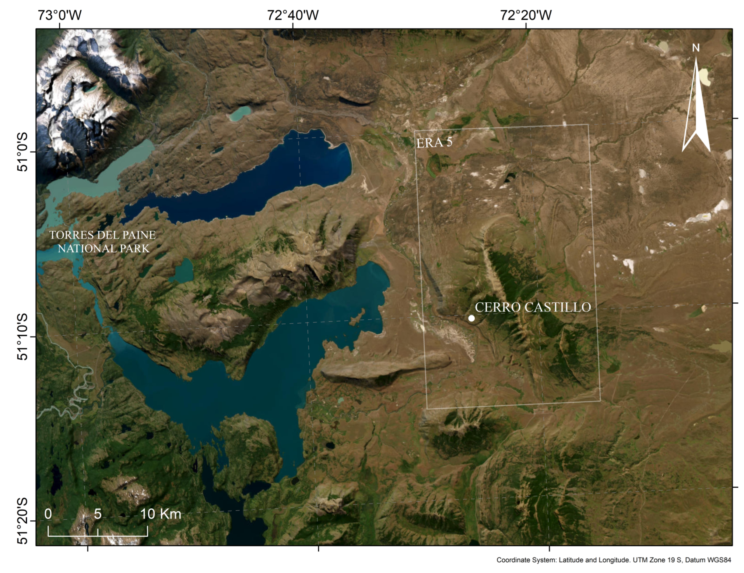
2.1. Area of Study

By its location and extension, SSA is a key region for the study of the SWW because it is the only continental landmass that covers the entire latitudinal range of this wind belt. Particularly, the area of study is located in the vicinity of Torres del Paine National Park (Figure 1), an area of southwestern Patagonia (~51° S) that is known to be in the present-day core of this wind belt [11].
Due to the topography of Patagonia, the SWW controls the cloudiness and rainfall on the western flank of the Andes [12]. Consequently, as already mentioned above, this area is characterized by a hyper-humid climate with extremely high precipitation rates that are very sensitive to any change in strength and/or latitudinal position of this wind belt.
Southern Patagonia has several lakes of glacial origin that have recorded climatic variations for the last thousands of years (e.g., [13,15]). Lacustrine cores have been used to propose wind reconstructions based on indirect records of wind intensity, such as changes in rainfall (e.g., [16,17,18]), vegetation patterns (e.g., [19,20]), fire history (e.g., [21]), or sea spray (e.g., [22]), all of which were assumedly driven by variations in the strength and latitudinal location of the SWW. So far, although promising qualitative (e.g., [22,23,24]) and quantitative (e.g., [14]) results were obtained in other regions, there has been no direct (i.e., based on aeolian particles) reconstruction of the wind variability in Southern Patagonia. The results of the present work constitute a stepping stone for future studies whose aim will be to reconstruct the history of the SWW from the aeolian content of the sediments of a selection of western Patagonian lakes.

2.2. Available Data

The recent work by [12] evidenced the consistency between the ERA5 reanalyzed surface winds and those measured at Cerro Castillo meteorological station, located in southwestern Patagonia (~51° S; Figure 1). This means that the ERA5 products can serve as a reference for analyzing the variability of the westerly winds in the area. Their advantage is that they are available for close to 50 years, against only a few years for the measurements of the Cerro Castillo station. Thus, in this work we take the data from this reanalysis to be representative of the winds in the study area.
ERA5 is the fifth generation of atmospheric reanalysis produced by the European Centre for Medium-Range Weather Forecast Reanalysis (ECMWF). It has replaced the very popular ERA-Interim reanalysis. The ERA5 surface wind is provided at the hourly resolution, the time series extend from the year 1959 to present time, and the horizontal resolution is 0.25° × 0.25° [25]. The data used in this work were downloaded from the Copernicus Climate Data Store (https://cds.climate.copernicus.eu/, accessed on 11 July 2022).

2.3. Quantification of the Strong Wind Anomalies

Wind erosion is a non-linear process that occurs only when wind speed is larger than the so-called erosion threshold [26], then its magnitude increases as the third power of the wind speed ([27] and references therein). Therefore, the cumulated rate of erosion in a given area is directly controlled by the frequency of the strong winds in this area.
In the present work, the quantification of this frequency relies first on the calculation of the number (Nstw) of strong winds in sliding windows of 3-month width. These strong winds are defined as those exceeding the 90th percentile (4.30 m s−1) of the hourly winds in the 1980–1989 period, arbitrarily selected as the reference. As the wind itself, Nstw follows a clear seasonal cycle with more (less) strong winds in austral summer (winter). A sinusoidal function is adjusted to represent the seasonal cycle of the reference period, and subtracting it from Nstw yields a number of ‘anomalies’ (Nanom). Positive (negative) Nanom characterize an enhancement (reduction) in the frequency of strong winds in a given period of 3 months, centered on each month of the year.
Keeping in mind that the objective of this study is to explore the possibility of reconstructing the wind history over several thousand years from the characteristics of aeolian particles found in sediment cores, and that the temporal resolution of these cores should be yearly in the best of cases, there is no point in taking the monthly and seasonal variations into account. Therefore, in our research of a correlation between Nanom and the large-scale modes of variability we will adopt a temporal resolution ranging from 1 to 9 years, which is more in keeping with the expected resolution of the sediment cores.

2.4. SAM

The Southern Annular Mode (SAM) is primarily an internal mode of climate variability that describes the north–south oscillation of the large-scale westerly wind belt in the extratropical SH (i.e., around Antarctica) [28,29,30]. The variations in the position and strength of this belt have significant impacts on the weather and climate in the SH, from the mid-latitude regions to Antarctica (for a review, see [31]), and serve to distinguish the positive (stronger winds and more poleward position of the core of the belt) and negative (weaker winds displaced toward the Equator) of the SAM [32].
The physical origin of the zonal winds in the extratropical latitudes results from the existence of a pressure gradient between the latitudes 40° (high) and 65° (low); consequently, a series of SAM indices based on the anomalies of geopotential height or pressure at sea-, or higher, levels were proposed in the literature (e.g., [7,29,33,34,35]). These indices differ in their definition, the type and source of the climate variables used to calculate them, and the time period over which they are retrieved. In their comparison of the most frequently used indices, ref [36] showed that the index proposed by [33] agreed quite well (R2 = 0.903) with the index of the National Oceanic and Atmospheric Administration (NOAA) that they had selected as their reference. Among the advantages of Marshall’s index, used to characterize the evolution of the SAM in the present study, one can cite the fact that it is: (1) based on actual observations performed at experimental stations and is, therefore, not affected by the uncertainties inherent to the pre-satellite era [33,37]; (2) available as of 1957 at the monthly resolution; (3) updated regularly by the British Antarctic Survey. The time series of the SAM index used in this work was downloaded from their website (https://www.bas.ac.uk, accessed on 4 May 2022).

2.5. ENSO and the Decadal Oscillations (IPO, PDO)

Several climate patterns involving fluctuations in the sea surface temperature (SST) have been identified in the Pacific Ocean. The most famous one is the El Niño–Southern Oscillation (ENSO), which is characterized by positive (El Niño) and negative (La Niña) phases corresponding to warm and cold anomalies of the SST, respectively, in the tropical Pacific Ocean. ENSO is usually considered to be a short-term pattern in the sense that it mainly occurs on scales of 2 to 7 years [38], and that its phases typically last only a few months. However, this variability is superimposed onto the weaker low-frequency variability of the decadal or multidecadal type [39,40,41].
A series of ENSO indices have been defined in the literature and are available for download from the website of the NOAA (https://psl.noaa.gov/data/climateindices/ (accessed on 4 May 2022)). Among these, we selected the BEST index [42] that combines the Nino 3.4 index and the Southern Oscillation Index (SOI, the pressure difference between Tahiti and Darwin). The BEST index is available at the monthly resolution as of January 1948. Its advantage is that, by incorporating the SOI, atmospheric processes which were neglected in Nino 3.4 are taken into account.
Besides ENSO, other modes of variability—also characterized by variations in the SST—have been identified in the Pacific region. However, their cycles can last several decades. This is the case for the Interdecadal Pacific Oscillation (IPO) [43,44], which is actually a tripole with a center of action in the north Pacific, one in the equatorial region, and one in the South Pacific [45]. The Pacific Decadal Oscillation (PDO) is closely related to the IPO and can be regarded as its North Pacific node [35,46]. The PDO has two phases: a positive one, during which the sea surface temperatures in the North Pacific are warmer than average; and a negative one, during which they are cooler than average. Because of this similarity with ENSO, the PDO has often been qualified as ENSO-like [47], but one first key difference between ENSO and PDO is the timescale of their oscillations. The second difference is that ENSO has a strong impact on the climate of the tropical Pacific and adjacent regions, whereas the PDO was initially considered to affect mostly the climate and ecosystems of the mid-latitude regions of the northern hemisphere, such as North America and Asia [48,49,50,51]. However, a series of more recent studies demonstrated that the PDO also has significant climate effects in the mid latitudes of the southern hemisphere, particularly in South America (e.g., [5,52,53,54]).
The PDO index of the Joint Institute for the Study of the Atmosphere and Ocean (JISAO), regularly updated and available at a monthly resolution, as of January 1900, was also downloaded from the NOAA website (https://psl.noaa.gov/gcos_wgsp/Timeseries/Data/pdo.long.data (accessed on 4 May 2022).

2.6. Quantification of the Correlation between the Wind Speed Anomalies and the Oscillations

The common period of availability for the ERA5 products, from which Nanom is calculated, and the SAM, PDO, and ENSO indices begins in January 1959. As mentioned above, the high-frequency (monthly and seasonal) variability of these time series was filtered using sliding averages calculated over windows of increasing (1, 3. 5, 7, and 9 years) widths.
The strength of the correlation between the four time series can be quantified by the means Pearson’s coefficient of correlation (R), or its square, which is the coefficient of determination (R2). The Principal Component Analysis (PCA; [55]) can also be used to investigate the statistical links between the times series. This procedure identifies which linearly independent combinations of the 4 variables are more apt to explain the variance in the whole dataset. These combinations are called principal components (PC) or factors (F). In this work, the XLstat PCA software was used.

3. Results

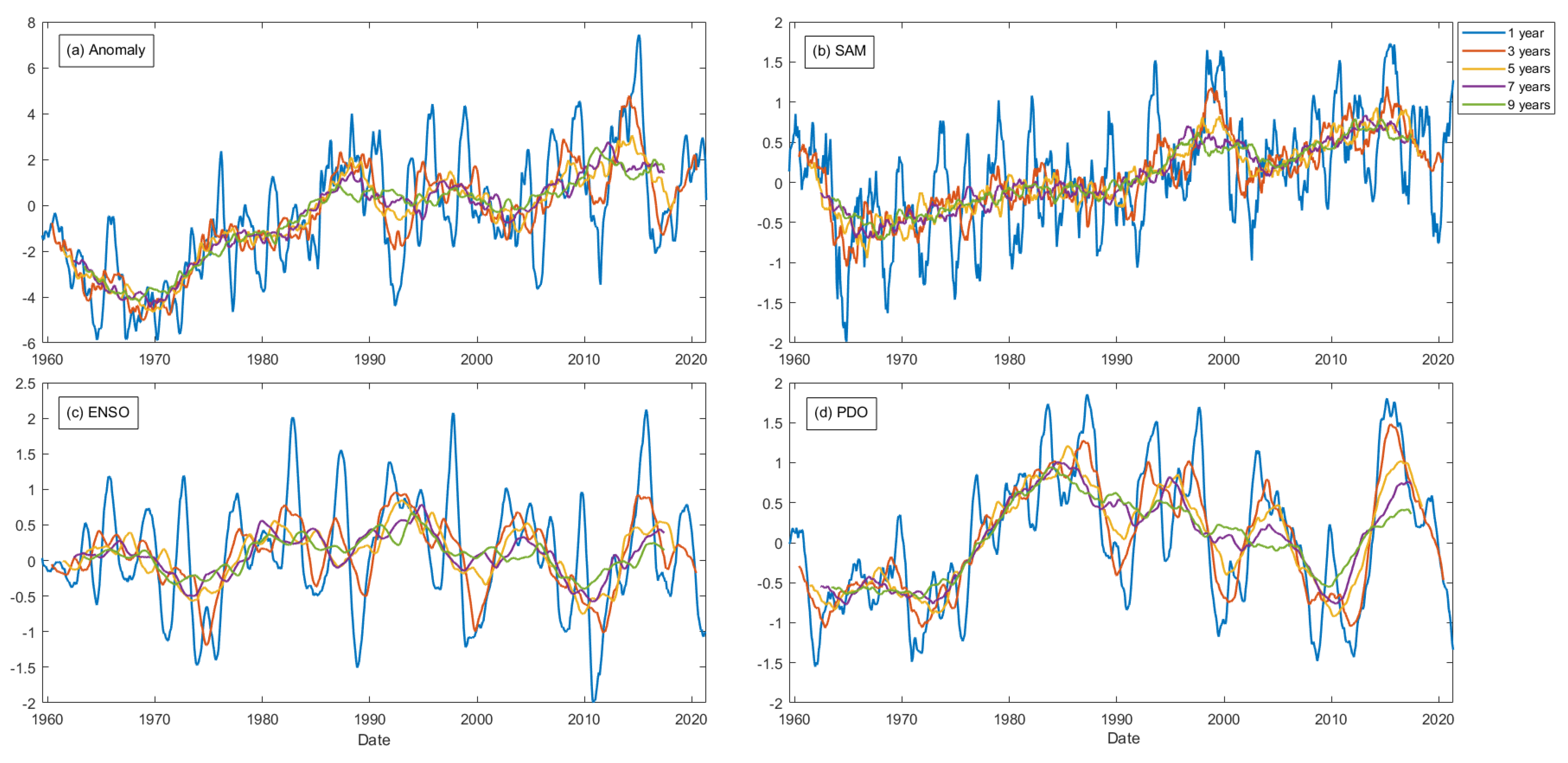
3.1. Time Series of Wind Speed, SAM, ENSO, and PDO at Different Temporal Resolutions

Figure 2 displays the temporal evolution between 1959 and 2021 of the: (a) anomalies of strong winds, (b) SAM, (c) ENSO, (d) PDO indices. On each plot, the results obtained using the five different widths of moving windows are reported.
The wind speed anomalies and the SAM, ENSO, and PDO indices are all characterized by an important interannual variability that is increasingly smoothed out by averaging over durations of 3 to 9 years. This averaging makes it easier to distinguish similarities in the trends of wind anomaly variation (Figure 2a) and the SAM (Figure 2b). Both decrease from 1959 to 1968 and increase afterwards. Reconstructions of the SAM’s evolution over the last century suggest that the marked increase observed in summer after the early 1970s is unprecedented [37]; this can been attributed to external forcing resulting from the combined effects of ozone layer depletion [56,57,58] and increased greenhouse concentrations in the atmosphere [59,60].
As proposed by [12], this commonality of behavior suggests that, although defined at a large scale, the SAM index could be well correlated to the variability of the winds in western Patagonia. Conversely, the regional winds of the southern tip of South America could be a useful proxy for the SAM variations. The strength of this correlation will be quantified more precisely in the following subsection.
For ENSO (Figure 2c) and the PDO (Figure 2d), there is no significant average trend in the indices over the whole 1959–2021 period. The main difference between the two lies in the fact that the frequencies involved in the variability of the ENSO are larger than those of the PDO. Therefore, after averaging over durations of 5 years or more there is an important levelling of the temporal variability of the ENSO index, whereas a clear decadal cycle of the PDO (with maximum positive phase around 1984, and negatives ones before 1972 and around 2010) can still be observed in the 9y sliding averages.

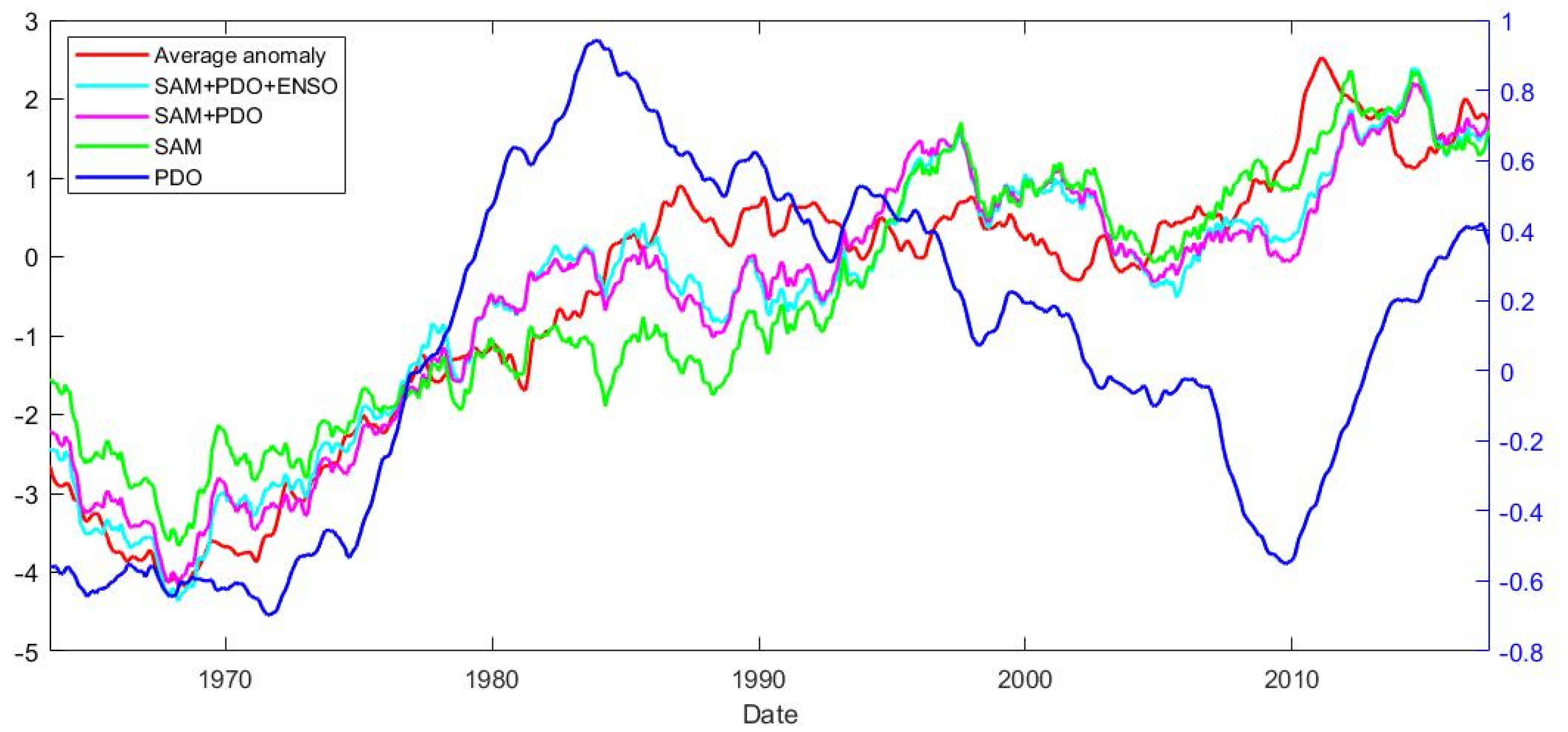
3.2. Correlation between Wind Speed Anomalies and the Oscillations

Over the period of study, more than 750 monthly values for the strong wind anomalies, SAM, ENSO, and PDO indices averaged over 1, 3, 5, 7, and 9 years are available. The principal component analysis applied to these five time series shows that, independent of the duration of the averaging period, two factors are enough to explain 78% (1y averaging) to 92% (7 and 9y averaging) of their variability. The first factor (F1) mostly combines the anomalies and the SAM, whereas the second one (F2) associates ENSO and the PDO. This strong correlation between the anomalies and the SAM on the one hand, and ENSO and the PDO on the other, can also be illustrated by the means of Pearson’s correlation coefficient (R, Table 1). R is the largest between the strong wind anomalies and SAM (from 0.672 to 0.870 for 3 and 9 y averages, respectively). The fact that R increases with the width of the averaging window suggests that taking into account the high-frequency variability of the SAM reduces the correlation between it and the anomalies. In other words, a retrieval of the SAM variations from the times series of wind anomalies is expected to provide better results at multi-year than at yearly resolutions. The data of Table 1 also confirm that the ENSO and PDO are relatively strongly correlated (R between 0.708 and 0.725), and that this independent of the averaging duration. Conversely, with an R very close to nil, the SAM is practically insensitive to the ENSO fluctuations. Finally, in addition to the SAM, the anomalies are found to be significantly correlated to the PDO (0.368 < R < 0.553). Although much less strongly, they also seem to depend on the ENSO index, but only for averaging durations of at least 9 years (R = 0.167). These observations suggest that only the low-frequency (decadal) variability of ENSO, similar to that of the PDO, could have a significant impact on the wind anomalies in western Patagonia.

3.3. Modelling of the Wind Speed Anomalies

Figure 2a,b, and the results of Table 1, indicate that the anomalies are primarily correlated to the SAM. The simplest way of representing this correlation mathematically is by the means of a linear expression:
Nanom = N0 + aSAM
However, to account for the dependence of the number of strong wind anomalies to the PDO and, although to a lesser degree, the ENSO, Equation (1) can be completed with the addition of two linear terms representing this dependence. Finally, this leads to:
Nanom = N0 + aSAM + bPDO + cENSO
In this equation, N0 represents the average number of anomalies in a period of 3 months, should the SAM, PDO, and ENSO indices be nil in the period of study (1959–2021). N0 could be either positive or negative. Conversely, a, b, and c quantify the sensitivity of Nanom to the variations of the SAM, PDO, and ENSO, respectively. Because Nanom clearly increases with the SAM, a is expected to be positive.
In this simple model, N0 and the 3 constants a, b, and c are unknown. Their values can be obtained by the means of a least square iterative routine providing the best possible fit for Equation (2) to the actual data derived from ERA5. This adjustment can be done for the 5 widths of averaging windows already considered previously. In each case, the quality of the adjustment is denoted by R2, and by the slope and vertical intercept of the plot of the modelled Nanom against the observed ones. Finally, the interest of including or not, the corrective terms corresponding to the PDO and/or ENSO effects can be evidenced by forcing either b or c (no PDO or no ENSO effect), or both of them (no PDO and no ENSO effect) to be 0. The results of these experiments are summarized in Table 2.
The slopes closest to 1, the lowest vertical intercepts, and the largest R2 are obtained with the complete form of Equation (2), which is to say by taking the PDO and ENSO into consideration, for windows of widths above 5 years. At smaller widths, the quality of the results degrades rapidly. Indeed, the slope and R2 both become less than 0.6 for 3y of averaging and even worse (<0.3) for 1y, which explains why the latter results are not reported in Table 2.
At the 9-year resolution, the results are not significantly worse when the ENSO effect is not taken into account than when it is. For instance, the slope remains very close to 0.87, the vertical intercept to −0.07, and R2 to 0.87 when the adjustment of Equation (2) is performed with a nil c. Conversely, omitting the PDO effect by forcing b to 0 has a direct impact on these three indicators. Even at the 7 and 9-year resolutions, for which the model still yields the best results, the slope and R2 do not exceed 0.76, and the vertical intercept increases in absolute value. These tests confirm that, if the strong wind anomalies in the region of study are primarily driven by the variations of the SAM, there is also a significant effect of the PDO. More precisely, the number of strong wind anomalies tends to be larger during the positive phases of the PDO than during the negative ones, which is consistent with the positive sign of b. Conversely, the effect of ENSO on these anomalies is, at best, a second order one when the largest widths of averaging windows (7 and 9-year) are considered. For the sake of illustration, Figure 3 compares the evolutions of the 9-year anomalies modeled by Equation (2) to the ERA5 time series, when accounting for the ENSO and PDO effects or not.
Interestingly, neglecting the ENSO effect has the largest impact on the performance of the model at the smallest temporal resolutions (3 and 5 years). For instance, when setting c to 0, R2 drops by 0.06 (from 0.57 to 0.51) at the 3-year resolution, compared to the 0.01 reduction observed for the 9-year averaging.

4. Discussion

In this study, we have quantified the impact of the SAM, PDO, and ENSO variations on the number of strong wind anomalies in western Patagonia and found that this number is primarily controlled by the variations of the SAM. Evidencing this dominant effect was undoubtedly facilitated by the fact that the SAM is characterized by an important increase in the period of study (1959–2021). A simple linear model simulating the variations of Nanom from only those of the SAM yields the best results after filtering the data over several years (R2 = 0.73 and 0.76 for 7 and 9 years, respectively). This indicates that the high-frequency (interannual) variability of Nanom does not directly reflect that of the SAM.
The predictions of the linear model are significantly improved after incorporating the effects of the PDO and the ENSO. Again, the quality of the model is optimal after averaging over more than 5 years and, in this case, the ENSO effect can be neglected.
The influence of the width of the averaging windows suggests that the strong wind anomalies in the high latitudes of Chilean Patagonia are sensitive to the quasi-decadal variations of the SAM and PDO, but not directly to the interannual ones. This is consistent with the minor effect of ENSO, in which the interannual variability largely prevails. A possible explanation for this lack of sensitivity to the high-frequency variations could be that the Patagonian winds react with a delay of several weeks or months to the variations of the PDO and ENSO oscillations, and that the influence of this time lag vanishes after averaging over durations of several years.
For evidencing this teleconnection between the decadal Pacific oscillation and the Patagonian winds, we have selected the PDO index. Among the most important reasons for this choice, one can mention that the PDO is widely documented in the literature, its index is regularly updated, and some studies suggested that it could have impacts included in the high latitudes of the SH. It was beyond the scope of the current study to check this; however, because of the strong correlation tying the PDO and the IPO and the fact that they are both characterized by similar decadal variations, it is highly probable that had the PDO been replaced by the IPO in Equation (2) similarly good results would also have been obtained. In other words, Nanom appears to be a good proxy for the combination of the SAM and the decadal oscillations of the Pacific area, the latter being represented either by the PDO (as in the current study) or by the IPO.

5. Summary and Conclusions

In this study we have performed a statistical analysis of the correlation existing between the strong wind anomalies (Nanom) of the southwestern Patagonia area and various indices (SAM, PDO, ENSO) characterizing the large-scale variability of the Pacific Ocean region. After application of a multiyear (>5 years) filtering, the results confirm the existence of strong teleconnections between these anomalies and the SAM. The PDO also plays a significant role, indicating that the temporal variations in the strong winds of southwestern Patagonia reflect the decadal oscillations of the Pacific region. Conversely, ENSO has practically no detectable effect on Nanom.
Nanom increases primarily with the SAM and also during the positive phases of the PDO. When compared to the observations, the simple linear model proposed to represent the dependence of Nanom on the SAM and PDO (Equation (2)) performs quite well (R2 = 0.86, slope = 0.86). This confirms the interest of using the variations in the strong-wind anomalies of southwestern Patagonia as a quantitative proxy for much larger-scale decadal modes of variability affecting the Pacific Ocean region.
These strong winds are the main drivers of wind erosion, and their frequency is directly reflected by the characteristics (quantity and size-distribution) of the content in aeolian particles from the sediments of southwestern Patagonia lakes. Therefore, the results of this work open new avenues of investigation for the reconstruction and study of past SWW changes, as well as of the modes of variability that influenced them.

Author Contributions

C.G.-F.: Conceptualization, Investigation, Methodology, Writing, Review and Editing. V.F.-A.: Conceptualization, Writing, Review and Editing, Project administration, Funding acquisition. S.C.A.: Conceptualization, Formal analysis, Methodology, Writing-Original Draft preparation, Review and Editing. All authors have read and agreed to the published version of the manuscript.

Funding

All authors were supported by Fondecyt grant no. 1191942; C. G.-F. is also funded by the ANID/Scholarship Program/Magister Nacional/2021-22210497. V. F.-A. was also supported by IRD through CHARISMA Project (JEAI-IRD-France/JE0ECCHARI).

Institutional Review Board Statement

Not applicable.

Informed Consent Statement

Not applicable.

Data Availability Statement

Data of ERA5 is available online at Copernicus Climate Data Store (https://cds.climate.copernicus.eu/, accessed on 11 July 2022).

Acknowledgments

This research was funded by Fondecyt grant no. 1191942 from National Agency for Research and Development (ANID) and support of IRD. This work is part of the Scientific Plan of the ANDEX/GEWEX Regional Hydroclimatic Program (https://www.gewex.org/project/andex/ (accessed on 13 February 2023)). V.F.-A. also acknowledges the support from IRD through CHARISMA Project (JEAI-IRD-France/JE0ECCHARI).

Conflicts of Interest

The authors declare no conflict of interest.

References

  1. Le Quéré, C.; Rödenbeck, C.; Buitenhuis, E.T.; Conway, T.J.; Langenfelds, R.; Gomez, A.; Labuschagne, C.; Ramonet, M.; Nakazawa, T.; Metzl, N.; et al. Saturation of the Southern Ocean CO2 sink due to recent climate change. Science 2007, 316, 1735–1738. [Google Scholar] [CrossRef] [PubMed] [Green Version]
  2. Hodgson, D.; Sime, L. Southern westerlies and CO2. Nat. Geosci. 2010, 3, 666–667. [Google Scholar] [CrossRef]
  3. Sigman, D.M.; Hain, M.P.; Huag, G.H. The polar ocean and glacial cycles in atmospheric CO2 concentration. Nature 2010, 466, 47–55. [Google Scholar] [CrossRef]
  4. Garreaud, R.; Lopez, P.; Minvielle, M.; Rojas, M. Large-scale control on the Patagonian climate. J. Clim. 2013, 26, 215–230. [Google Scholar] [CrossRef]
  5. Garreaud, R.N.; Vuille, M.; Compagnucci, R.; Matengo, J. Present-day South American climate. Palaeogeogr. Palaeocl. 2009, 281, 180–195. [Google Scholar] [CrossRef]
  6. Sime, L.C.; Kohfeld, K.E.; Le Quere, C.; Wolff, E.; de Boer, A.M.; Graham, R.M.; Bopp, L. Southern Hemisphere westerly wind changes during the Last Glacial Maximum: Model-data comparison. Quat. Sci. Rev. 2013, 64, 104–120. [Google Scholar] [CrossRef] [Green Version]
  7. Thompson, D.W.; Wallace, J.M. Annular modes in the extratropical circulation. Part I: Month-to-month variability. J. Clim. 2000, 13, 1000–1016. [Google Scholar] [CrossRef]
  8. Thompson, D.W.J.; Solomon, S. Interpretation of recent Southern Hemisphere climate change. Science 2002, 296, 895–899. [Google Scholar] [CrossRef] [Green Version]
  9. Marshall, G.J.; Stott, P.A.; Turner, J.; Connolley, W.M.; King, J.C.; Lachlan-Cope, T.A. Causes of exceptional atmospheric circulation changes in the Southern Hemisphere. Geophys. Res. Lett. 2002, 31, L14205. [Google Scholar] [CrossRef]
  10. Gillet, N.; Thompson, D. Simulation of Recent Southern Hemisphere Climate Change. Science 2003, 302, 273–275. [Google Scholar] [CrossRef] [Green Version]
  11. Browne, I.M.; Moy, C.M.; Riesselman, C.R.; Neil, H.L.; Curtin, L.G.; Gorman, A.R.; Wilson, G.S. Late Holocene intensification of the westerly winds at the subantarctic Auckland Islands (51° S), New Zealand. Clim. Past 2017, 13, 1301–1322. [Google Scholar] [CrossRef] [Green Version]
  12. Gómez-Fontealba, C.; Flores-Aqueveque, V.; Alfaro, S.C. Variability of the Southwestern Patagonia (51° S) winds in the recent (1980–2020) period. Implications for past wind reconstructions. Atmosphere 2017, 13, 206. [Google Scholar] [CrossRef]
  13. Moreno, P.I.; Vilanova, I.; Villa-Martínez, R.; Dunbar, R.B.; Mucciarone, D.A.; Kaplan, M.R.; Garreaud, R.D.; Rojas, M.; Moy, C.M.; Pol-Holz, R.D.; et al. Onset and Evolution of Southern Annular Mode-Like Changes at Centennial Timescale. Sci. Rep. 2018, 8, 3458. [Google Scholar] [CrossRef] [PubMed] [Green Version]
  14. Flores-Aqueveque, V.; Alfaro, S.; Vargas, G.; Rutllant, J.A.; Caquineau, S. Aeolian particles in marine cores as a tool for quantitative high-resolution reconstruction of upwelling favorable winds along coastal Atacama Desert, Northern Chile. Prog. Oceanogr. 2015, 134, 244–255. [Google Scholar] [CrossRef]
  15. Moy, C.; Moreno, P.; Dunbar, R.; Kaplan, M.; Francois, J.-P.; Villalba, R.; Haberzettl, T. Climate change in Southern South America during the last two millennia. In Past Climate Variability in South America and Surrounding Regions, Developments in Paleoenvironmental Research; Springer Science & Business Media: Berlin/Heidelberg, Germany, 2009; pp. 353–393. [Google Scholar]
  16. Jenny, B.; Valero-Garcés, B.; Villa-Martínez, T.; Urrutia, R.; Geyh, M. and Veit, H. Early to Mid-Holocene Aridity in Central Chile and the Southern Westerlies: The Laguna Aculeo Record (34° S). Quat. Res. 2002, 58, 160–170. [Google Scholar] [CrossRef]
  17. Lamy, F.; Kilian, R.; Arz, H.; Francois, J.P.; Kaiser, J.; Prange, M.; Steinke, T. Holocene changes in the position and intensity of the southern westerly wind belt. Nat. Geosci. 2010, 3, 695–699. [Google Scholar] [CrossRef] [Green Version]
  18. Bertrand, S.; Hughen, K.; Sepúlveda, J.; Pantoja, S. Late Holocene covariability of the southern westerlies and sea surface temperature in northern Chilean Patagonia. Quat. Sci. Rev. 2014, 105, 195–208. [Google Scholar] [CrossRef]
  19. Moy, C.M.; Dunbar, R.B.; Moreno, P.I.; François, J.P.; Villa-Martínez, R.; Mucciarone, D.M.; Guilderson, T.O.; Garreaud, R.D. Isotopic evidence for hydrologic change related to the westerlies in SW Patagonia, Chile, during the last millennium. Quat. Sci. Rev. 2008, 27, 1335–1349. [Google Scholar] [CrossRef]
  20. Moreno, P.I.; François, J.P.; Villa-Martínez, R.; Moy, C.M. Millennial-scale variability in Southern Hemisphere westerly wind activity over the last 5000 years in SW Patagonia. Quat. Sci. Rev. 2009, 28, 25–38. [Google Scholar] [CrossRef]
  21. Moreno, P.I.; Vilanova, I.; Villa-Martínez, R.; Garreaud, R.D.; Rojas, M.; De Pol-Holz, R. Southern Annular Mode-like changes in southwestern Patagonia at centennial timescales over the last three millennia. Nat. Commun. 2014, 5, 4375. [Google Scholar] [CrossRef] [Green Version]
  22. Saunders, K.; Roberts, S.; Perren, B.; Butz, C.; Sime, L.; Davies, S.; Van Nieuwenhuyze, W.; Grosjean, M.; Hodgson, D. Holocene dynamics of the Southern Hemisphere westerly winds and possible links to CO2 outgassing. Nat. Geosci. 2018, 11, 650–655. [Google Scholar] [CrossRef] [Green Version]
  23. Briceño-Zuluaga, F.J.; Sifeddine, A.; Caquineau, S.; Cardich, J.; Salvatteci, R.; Gutierrez, D.; Ortlieb, L.; Velazco, F.; Boucher, H.; Machado, C. Terrigenous material supply to the Peruvian central continental shelf (Pisco, 14° S) during the last 1000 years: Paleoclimatic implications. Clim. Past 2016, 12, 787–798. [Google Scholar] [CrossRef] [Green Version]
  24. Warrier, A.; Pednekar, H.; Mahesh, B.S.; Mohan, R.; Gazi, S. Sediment grain size and surface textural observations of quartz grains in late quaternary lacustrine sediments from Schirmacher Oasis, East Antarctica: Paleoenvironmental significance. Polar Sci. 2016, 10, 89–100. [Google Scholar] [CrossRef]
  25. Hersbach, H.; Bell, B.; Berrisford, P.; Hirahara, S.; Horányi, A.; Muñoz Sabater, J.; Nicolas, J.; Peubey, C.; Radu, R.; Schepers, D.; et al. The ERA5 global reanalysis. Q. J. R. Meteorol. Soc. 2020, 146, 1999–2049. [Google Scholar] [CrossRef]
  26. Bagnold, R.A. The Physics of Blown Sand and Desert Dunes, 1st ed.; Methuen & Co.: London, UK, 1941. [Google Scholar]
  27. Marticorena, B.; Bergametti, G. Modelling the atmospheric dust cycle. J. Geophys. Res. 1995, 100, 16415–16430. [Google Scholar] [CrossRef] [Green Version]
  28. Rogers, J.C.; Van Loon, H. Spatial variability of sea level pressure and 500 mb height anomalies over the Southern Hemisphere. Mon. Weather. Rev. 1982, 110, 1375–1392. [Google Scholar] [CrossRef]
  29. Gong, D.; Wang, S. Definition of Antarctic oscillation index. Geophys. Res. Lett. 1999, 26, 459–462. [Google Scholar] [CrossRef] [Green Version]
  30. Limpasuvan, V.; Hartmann, D.L. Eddies and the annular modes of climate variability. Geophys. Res. Lett. 1999, 26, 3133–3136. [Google Scholar] [CrossRef] [Green Version]
  31. Fogt, R.L.; Marshall, G.J. The Southern Annular Mode: Variability, trends, and climate impacts across the Southern Hemisphere. Wiley Interdiscip. Rev. Clim. Chang. 2020, 11, e652. [Google Scholar] [CrossRef]
  32. Thompson, D.W.J.; Solomon, S.; Kushner, P.J.; England, M.H.; Grise, K.M.; Karoly, D.J. Signatures of the Antarctic ozone hole in Southern Hemisphere surface climate change. Nat. Geosci. 2011, 4, 741–749. [Google Scholar] [CrossRef]
  33. Marshall, G.J. Trends in the Southern Annular Mode from observations and reanalyses. J. Clim. 2003, 16, 4134–4143. [Google Scholar] [CrossRef]
  34. Fan, K.; Wang, H.J. Antarctic oscillation and the dust weather frequency in North China. Geophys. Res. Lett. 2004, 31, L10201. [Google Scholar] [CrossRef] [Green Version]
  35. Visbeck, M. A station-based southern annular mode index from 1884 to 2005. J. Clim. 2009, 22, 940–950. [Google Scholar] [CrossRef] [Green Version]
  36. Ho, M.; Kiem, A.S.; Verdon-Kidd, D.C. The Southern Annular Mode: A comparison of indices. Hydrol. Earth Syst. Sci. 2012, 16, 967–982. [Google Scholar] [CrossRef] [Green Version]
  37. Jones, J.M.; Fogt, R.L.; Widmann, M.; Marshall, G.J.; Jones, P.D.; Visbeck, M. Historical SAM Variability. Part I: Century-Length Seasonal Reconstructions. J. Clim. 2009, 22, 5319–5345. [Google Scholar] [CrossRef] [Green Version]
  38. Wang, C.; Picaut, J. Understanding ENSO physics—A review. Earth’s Climate: The Ocean–Atmosphere Interaction. Geophys. Monogr. 2004, 147, 21–48. [Google Scholar]
  39. Lau, K.M.; Weng, H. Interannual, decadal–interdecadal, and global warming signals in sea surface temperature during 1955–97. J. Clim. 1999, 12, 1257–1267. [Google Scholar] [CrossRef]
  40. Cai, W.; Whetton, P.H.; Pittock, A.B. Fluctuations of the relationship between ENSO and northeast Australian rainfall. Clim. Dyn. 2001, 17, 421. [Google Scholar] [CrossRef]
  41. Philander, S.G.; Fedorov, A. Is El Niño sporadic or cyclic? Annu. Rev. Earth Planet. Sci. 2003, 31, 579–594. [Google Scholar] [CrossRef] [Green Version]
  42. Smith, C.A.; Sardeshmukh, P. The Effect of ENSO on the Intraseasonal Variance of Surface Temperature in Winter. Int. J. Climatol. 2000, 20, 1543–1557. [Google Scholar] [CrossRef]
  43. Folland, C.K.; Parker, D.E.; Colman, A.W.; Washington, R. Large Scale Modes of Ocean Surface Temperature Since the Late Nineteenth Century; Springer: Berlin/Heidelberg, Germany, 1999; pp. 73–102. [Google Scholar]
  44. Power, S.; Casey, T.; Folland, C.; Colman, A.; Mehta, V. Inter-decadal modulation of the impact of ENSO on Australia. Clim. Dyn. 1999, 15, 319–324. [Google Scholar] [CrossRef]
  45. Henley, B.J.; Gergis, J.; Karoly, D.J.; Power, S.; Kennedy, J.; Folland, C.K. A tripole index for the interdecadal Pacific oscillation. Clim. Dyn. 2015, 45, 3077–3090. [Google Scholar] [CrossRef]
  46. Folland, C.K.; Renwick, J.A.; Salinger, M.J.; Mullan, A.B. Relative influences of the interdecadal Pacific oscillation and ENSO on the South Pacific convergence zone. Geophys. Res. Lett. 2002, 29, 21-1–21-4. [Google Scholar] [CrossRef]
  47. Garreaud, R.D.; Battisti, D.S. Interannual (ENSO) and interdecadal (ENSO-like) variability in the Southern Hemisphere tropospheric circulation. J. Clim. 1999, 2, 2113–2123. [Google Scholar] [CrossRef]
  48. Mantua, N.J.; Hare, S.R.; Zhang, Y.; Wallace, J.M.; Francis, R.C. A Pacific interdecadal climate oscillation with impacts on salmon production. Bull. Am. Meteorol. Soc. 1997, 78, 1069–1079. [Google Scholar] [CrossRef]
  49. Mantua, N.J.; Hare, S.R. The Pacific Decadal Oscillation. J. Oceanogr. 2002, 58, 35–44. [Google Scholar] [CrossRef]
  50. Duffy, P.A.; Walsh, J.E.; Graham, J.M.; Mann, D.H.; Rupp, T.S. Impacts of large-scale atmospheric–ocean variability on Alaskan fire season severity. Ecol. Appl. 2005, 15, 1317–1330. [Google Scholar] [CrossRef] [Green Version]
  51. Di Lorenzo, E.; Cobb, K.M.; Furtado, J.C.; Schneider, N.; Anderson, B.T.; Bracco, A.; Alexander, M.A.; Vimont, D.J. Central pacific El Nino and decadal climate change in the North Pacific Ocean. Nat. Geosci. 2010, 3, 762–765. [Google Scholar] [CrossRef]
  52. Da Silva, G.A.M.D.; Drumond, A.; Ambrizzi, T. The impact of El Niño on South American summer climate during different phases of the Pacific Decadal Oscillation. Theor. Appl. Climatol. 2011, 106, 307–319. [Google Scholar] [CrossRef]
  53. Vuille, M.; Franquist, E.; Garreaud, R.; Lavado Casimiro, W.S.; Cáceres, B. Impact of the global warming hiatus on Andean temperature. J. Geophys. Res. Atmos. 2015, 120, 3745–3757. [Google Scholar] [CrossRef] [Green Version]
  54. Valdés-Pineda, R.; Cañón, J.; Valdés, J.B. Multi-decadal 40-to 60-year cycles of precipitation variability in Chile (South America) and their relationship to the AMO and PDO signals. J. Hydrol. 2018, 556, 1153–1170. [Google Scholar] [CrossRef]
  55. Wold, S.; Esbensen, K.; Geladi, P. Principal component analysis. Chemom. Intell. Lab. Syst. 1987, 2, 37–52. [Google Scholar] [CrossRef]
  56. England, M.H.; McGregor, S.; Spence, P.; Meehl, G.A.; Timmermann, A.; Cai, W.; Gupta, A.S.; McPhaden, M.J.; Purich, A.; Santoso, A. Recent intensification of wind-driven circulation in the Pacific and the ongoing warming hiatus. Nat. Clim. Chang. 2014, 4, 222–227. [Google Scholar] [CrossRef] [Green Version]
  57. Jones, J.M.; Gille, S.T.; Goosse, H.; Abram, N.J.; Canziani, P.O.; Charman, D.J.; Clem, K.R.; Crosta, X.; de Lavergne, C.; Eisenman, I.; et al. Assessing recent trends in high-latitude Southern Hemispheresurface climate. Nat. Clim. Chang. 2016, 6, 917–926. [Google Scholar] [CrossRef]
  58. Fogt, R.L.; Goergens, C.A.; Jones, J.M.; Schneider, D.P.; Nicolas, J.P.; Bromwich, D.H.; Dusselier, H.E. A twentieth century perspective on summer Antarctic pressure change and variability and contributions from tropical SSTs and ozone depletion. Geophys. Res. Lett. 2017, 44, 9918–9927. [Google Scholar] [CrossRef]
  59. Cai, W.; Collier, M.A.; Gordon, H.B.; Waterman, L.J. Strong ENSO variability and a Super-ENSO pair in the CSIRO Mark 3 coupled climate model. Mon. Weather. Rev. 2003, 131, 1189–1210. [Google Scholar] [CrossRef]
  60. Arblaster, J.M.; et Meehl, G.A. Contributions of external forcings to southern annular mode trends. J. Clim. 2006, 19, 2896–2905. [Google Scholar] [CrossRef]
Figure 1. Map of the study area showing the location of the Cerro Castillo meteorological station (white circle) and the corresponding grid (white rectangle) of the ERA5 reanalysis.
Atmosphere 14 00608 g001
Figure 2. Temporal evolution of the: (a) anomalies of strong winds (for the unit, see Section 2.2), (b) SAM, (c) ENSO, (d) PDO.
Atmosphere 14 00608 g002
Figure 3. Temporal evolution of the ERA5 strong wind anomalies (red curve) and of the anomalies yielded by Equation (2) when taking the SAM, PDO, and ENSO effects into account (cyan line). The width of the averaging window is 9 years. For the sake of comparison, the results obtained when neglecting the ENSO (magenta line), or both the PDO and ENSO (green line) effects, are also represented. The variations of the PDO are reported in blue and its values are reported on the right vertical axis.
Atmosphere 14 00608 g003
Table 1. Pearson’s coefficient of correlation (R) linking the times series of the strong wind anomalies, and the PDO, ENSO, and SAM indices.
Averaging3 Years5 Years
PDOENSOSAMAnomaliesPDOENSOSAMAnomalies
PDO10.7090.2210.36810.7120.2820.469
ENSO 1−0.038−0.001 1−0.0090.034
SAM 10.672 10.810
Anomalies 1 1
Averaging7 years9 years
PDOENSOSAMAnomaliesPDOENSOSAMAnomalies
PDO10.7080.2850.50510.7250.2910.553
ENSO 1−0.0210.070 1−0.0050.167
SAM 10.857 10.870
Anomalies 1 1
Table 2. Results of the adjustment of Equation (2) to the ERA5 data. The indicators (slope, vertical intercept, and R2) of the quality of this adjustment can be compared to those obtained when not taking into account the ENSO (c is forced to 0), or both the PDO and the ENSO (b = c = 0). The standard deviations (sd) of the slope and vertical intercept correspond to the 95% confidence interval.
SAMYesYesYes
PDOYesYesNo
ENSOYesNoNo
Years357935793579
N0−0.71−0.71−0.71−0.75−0.84−0.86−0.83−0.85−0.83−0.83−0.81−0.80
a2.452.983.273.382.753.313.563.562.993.653.934.00
b1.551.671.701.760.740.841.001.240000
c−1.56−1.77−1.66−1.360000.000000
Slope0.570.770.840.870.510.720.810.860.450.660.730.76
sd0.020.020.010.010.020.020.020.010.020.020.020.02
Intercept−0.27−0.14−0.09−0.07−0.31−0.17−0.11−0.08−0.34−0.20−0.15−0.13
sd0.040.030.030.020.040.030.030.030.040.040.030.03
R20.570.770.840.870.510.720.810.860.450.660.730.76
Disclaimer/Publisher’s Note: The statements, opinions and data contained in all publications are solely those of the individual author(s) and contributor(s) and not of MDPI and/or the editor(s). MDPI and/or the editor(s) disclaim responsibility for any injury to people or property resulting from any ideas, methods, instructions or products referred to in the content.

