Simulation and Analysis of the Influence of Sounding Rocket Outgassing on In-Situ Atmospheric Detection

Abstract

The Meridian Project’s sounding rocket mission uses a mass spectrometer to conduct in-situ atmospheric detection. In order to assess the influence of surface material outgassing and the attitude control jet on the spectrometer’s detection, a sounding rocket platform was modeled and simulated. Using the physical field simulation software COMSOL and the Monte Carlo method, this study investigated whether the gas molecules from the two cases could enter the in-situ atmospheric mass spectrometer’s sensor sampling port after colliding with the background atmosphere. The simulation results show that the influence of surface material outgassing on the in-situ atmospheric detection is very small, even under the conditions of medium solar activity and medium geomagnetic activity, while the influence of the attitude control jet on the in-situ atmospheric detection is large but can be reduced by reducing the low-altitude attitude control operation and decreasing the transmission probability. Through simulation optimization and according to engineering needs, increasing the nozzle outlet cross-sectional area, increasing the temperature of the gas used for attitude control, increasing the nozzle rotation angle, increasing the nozzle outlet angle, or increasing the nozzle center height can reduce the transmission probability. This model can simulate and analyze the influence of both surface material outgassing and attitude control jets on in-situ atmospheric detection, optimize relevant parameters, and provide new ideas for relevant work.

1. Introduction

Sounding rockets are a powerful method for the in-situ detection of the atmosphere and ionosphere at 20–200 km. This region is beyond the capability of sounding balloons and is too low for satellites to operate for long periods of time. This makes sounding rockets the best platform for collecting data and observing phenomena. Sounding rockets have the advantages of a simple structure, mature technology, low cost, and controllable risk; meanwhile, they are highly flexible and can be launched quickly for detection when solar activity and geomagnetic activity are intense. Therefore, developed countries, such as Europe [1,2,3,4,5] and the United States [6], as well as Japan [7] and India [8], have been actively developing sounding rockets and conducting missions at an early stage and have achieved many scientific results [9,10,11,12,13]. Today’s advanced international sounding rockets can even reach an altitude of 1000 km. Additionally, China began sounding rocket research in 1958, and three generations of sounding rockets have been developed in 50 years [14,15].

The Meridian Project, a major national scientific project, was started by the Chinese Academy of Sciences (CAS) in 2008. The Meridian Project is the most comprehensive, full-featured, and longest-spanning space environment ground-based monitoring network in the world [16,17]. Additionally, through the efforts of scientists from China and around the world, it has gradually developed into the International Meridian Circle Program [18]. The Meridian Project uses sounding rockets to conduct in-situ detection within the atmospheric environment at 20–320 km to complement ground-based detection, to explore the dynamical processes and mechanisms of the atmosphere, ionosphere, and solar-terrestrial space [19,20], and to provide the necessary environmental parameters for atmospheric science, scientific research [21,22] and engineering projects related to the atmosphere.

Spacecraft contamination has always been an important aspect to consider in spacecraft design and has been studied by many researchers [23,24,25,26,27]. Spacecraft contamination is mainly caused by particles of surface materials outgassing from platforms and payloads, as well as particles generated by thrusters and attitude control operations. Spacecraft contamination affects not only optical instruments but also in-situ mass spectrometers, especially in a thin atmosphere. For optical instruments [28], deposition of contamination can lead to degradation of instrument performance; for mass spectrometers [29,30,31], contamination does not degrade instrument performance but can produce significant background signals, especially for detection missions in thin atmospheres, which affect the reliability and authenticity of the detection results.

So far, many scholars have used simulation analysis [32,33,34,35,36], in-orbit monitoring [37], and adsorption [38,39] control to study spacecraft contamination. Sounding rocket missions are not very long (typically 5–20 min), and the detection region is the atmosphere. Therefore, simulation and analysis before missions are particularly important to address the issue of sounding rocket contamination. Simulation and analysis can be used to improve and optimize the structure and location of rockets and payloads and to filter noise from the result data after missions to reduce the effects of contamination. This paper focuses on the influence of surface material outgassing and the attitude control jet on the mass spectrometer used for in-situ atmospheric detection in the context of the Meridian Project sounding rocket mission and investigates whether the gas molecules from the above two cases can enter the mass spectrometer’s sensor sampling port after colliding with the background atmosphere. The physical field simulation software COMSOL is used to model and simulate the collision process with the Monte Carlo method to explore the influence of different solar and geomagnetic activities, and to support the development of the Meridian Project sounding rocket mission.

2. Theory and Methods

2.1. Gas Molecular Collision Model

Monte Carlo methods are often used to simulate collision processes. The direct simulation Monte Carlo (DSMC) method is suitable for solving the Boltzmann equation to study rarefied gas flow [32,40,41] and is relatively easy to apply in terms of programming effort and computational time. Additionally, atmospheric motion above 120 km can be regarded as free molecular flow, which is the equilibrium Maxwell distribution and can be described and calculated by the Boltzmann equation. DSMC uses a large number of simulated molecules (10⁴–10⁶ or more) and records the position, velocity, internal energy, and collision process of each simulated molecule, as well as its state after the collision, so as to simulate the complex physical phenomena of the atmosphere. Collisions between molecules are handled based on probability.

The surface material of the sounding rocket platform can adsorb gas molecules, which can escape when the altitude increases and the pressure decreases. The sounding rocket platform is controlled in flight by jetting gas, and these two cases of gas molecules will collide with the background atmosphere. In 1858, Clausius developed the elastic sphere model of gas molecules, introducing the average collision frequency, i.e., the average number of collisions of a molecule with other molecules per unit of time. This model simplifies molecular motion:

• The molecular repulsion range is set to a rigid sphere of diameter d;
• The collisions between molecules are elastic;
• The background molecules are approximately stationary;
• The incident molecules move at average speed $\overline{v}$.

The incident molecular A’s motion is shown in Figure 1. The cross-sectional area of the cylinder, i.e., the area of molecular collision, is $\sigma$. The distance traveled by A in time t is $\overline{v}t$. The numerical density of gas molecules in the background atmosphere is n. The total number of molecules centered in the cylinder, i.e., the number of molecules colliding with A, is $n\sigma \overline{v}t$. The average collision frequency is shown in Equation (1).

$$\overline{z}=\frac{n\sigma \overline{v}t}{t}=n\sigma \overline{v}$$

(1)

In 1860, Maxwell used probability statistics to derive the speed distribution function of equilibrium gas molecules, i.e., Maxwell’s distribution, and used the distribution to derive the relationship between average speed and absolute temperature, and modified Clausius’ formula, as shown in Equation (2):

$$\overline{z}=n\sigma \sqrt{({\overline{v}}_A{}^2+{\overline{v}}_B{}^2)}=n\pi d^2\sqrt{({\overline{v}}_A{}^2+{\overline{v}}_B{}^2)}$$

(2)

The diameter d is given by the Van der Waals radius of molecules; the average speed of background molecules is obtained from the Maxwell distribution; and different molecules’ numerical density in the background atmosphere is calculated using the NRLMSISE-00 model [42,43]. The NRLMSISE-00 model was developed by the U.S. Naval Laboratory based on satellite mass spectrometer data and incoherent scattering radar temperature measurements and is one of the most advanced and well-established empirical atmospheric models in the world, which is widely used in data analysis and simulation.

2.2. Surface Material Outgassing

Generally, any solid material can adsorb gas molecules. Additionally, when the solid material is placed in a high-vacuum environment, the gas will be desorbed and escape. According to the literature [44,45], Equation (3) is obtained, where q is the material outgassing rate in Pa·L/(s·cm²); C is the pumping speed in L/s for the pressure change (the following text uses m³/s as the unit); p₁ and p₂ are the values before and after the pressure change in Pa; and S is the surface area of the material in cm². According to the mission, the material outgassing rate is 533.2 × 10⁻⁶ Pa·L/(s·cm²).

$$q=\frac{C(p_1-p_2)}{S}$$

(3)

2.3. Attitude Control Jet

According to the mission, the attitude control uses a de Laval nozzle; its structure is shown in Figure 2, and its design parameters are shown in

Table 1. Design parameters of the de Laval nozzle.

Parameter	Value
Inlet radius	1.30 mm
Throat radius	0.75 mm
Outlet radius	2.60 mm
Outlet angle	30°

. The cold gas propulsion method is used, and the gas is nitrogen (N₂). From the principle of the de Laval nozzle, it is known that the gas speed is accelerated from subsonic to supersonic as the cross-sectional area of the nozzle outlet changes. The relationship is shown in Equation (4) and Figure 3, where γ is the adiabatic index (1.66 for monatomic molecules and 1.40 for diatomic molecules).

$$\frac{A^{*}}{A}={(\frac{\gamma +1}{2})}^{\frac{1}{\gamma -1}}Ma{(1-\frac{\gamma -1}{\gamma +1}M{a}^2)}^{\frac{1}{\gamma -1}}$$

(4)

According to aerodynamics, the speed of sound is calculated as shown in Equation (5), where γ is the adiabatic index (1.66 for monatomic molecules and 1.40 for diatomic molecules), R is the gas constant, T is the absolute temperature, and M is molar mass. Combining Table 1, Equation (4), and Equation (5), the speed of jetting N₂—whose temperature is 303 K—to the nozzle outlet in the mission design is about 765 m/s.

$$c=\sqrt{\gamma \frac{p}{\rho }}=\sqrt{\frac{\gamma RT}{M}}$$

(5)

2.4. Simulation Model

COMSOL Multiphysics (COMSOL) [46] is a powerful piece of physical field simulation software based on the finite element method that can be used to solve systems of partial differential equations to simulate physical phenomena and can be used to analyze electromagnetic, structural, fluid, heat transfer, and engineering problems. COMSOL’s free molecular flow module has been used to simulate and analyze spacecraft contamination [47,48,49]. However, the particle tracking module is better suited to deal with the collision process. The particle tracking module [50] supports the calculation of particle trajectories in fluid or electromagnetic fields, including particle–particle, particle–fluid, and particle–field interactions. The particle tracking module has a velocity reinitialization feature that applies random forces to particles during the simulation, allowing various Monte Carlo simulations to be performed. The module has collision nodes for adding random collisions, and further sub-nodes for elasticity, ionization, and excitation can be selected.

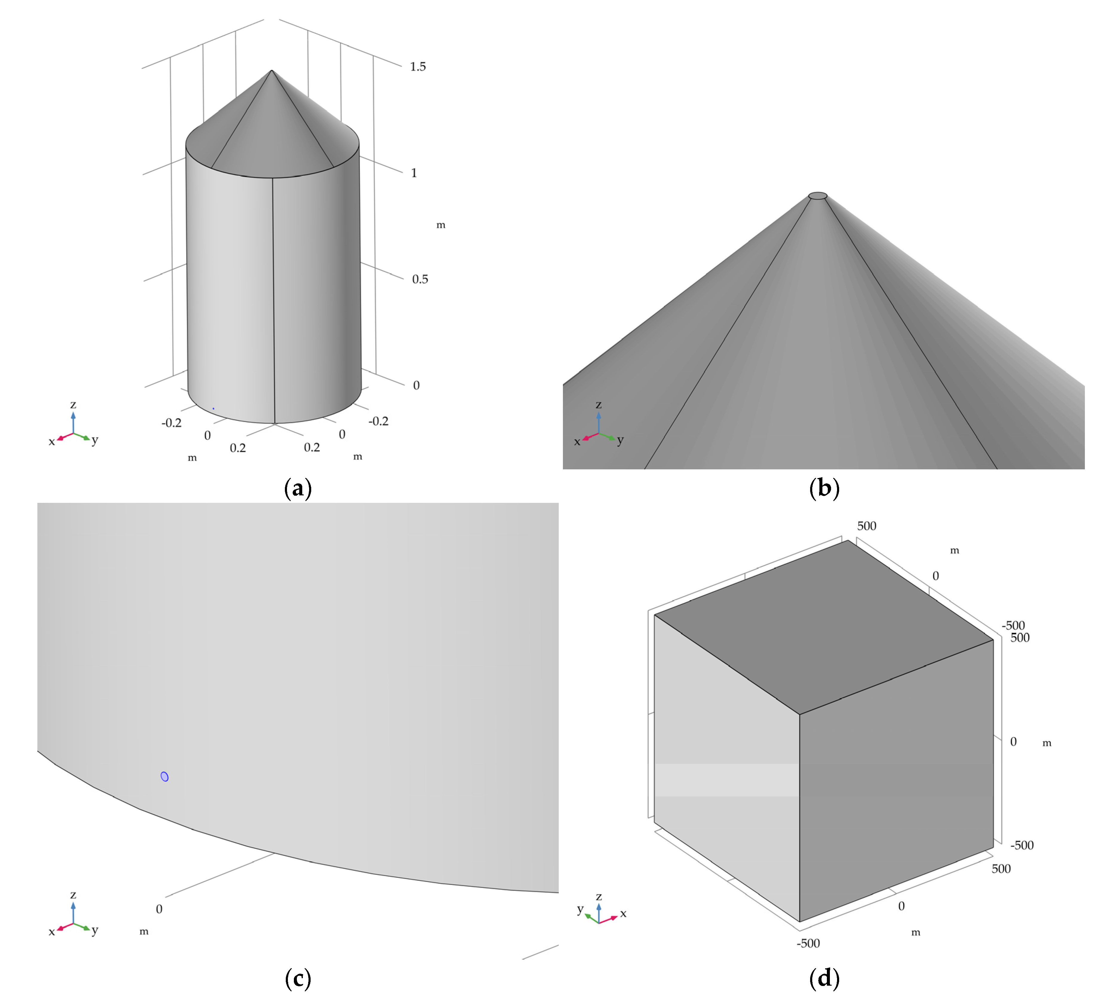
The flowchart of the building model is shown in Figure 4. The structure of the model is shown in Figure 5, and the geometrical parameters are shown in

Table 2. Geometric parameters of the model.

Domain	Parameter	Value
Frustum of a cone of platform	Top radius	2.50 mm
	Bottom radius	0.375 m
	Height	0.345 m
Cylinder of platform	Radius	0.375 m
	Height	1.115 m
The outlet of the de Laval nozzle of the platform	Radius	2.60 mm
	Center height	25 mm
Collision	Edge length	500 m

. The direction of the outer normal vector of the nozzle outlet is the same as the positive direction of the x-axis. Figure 5a is placed in the center of Figure 5d.

The particle tracking module was selected to simulate the collision process between the gas molecules from the outgassing or jet and the background atmosphere. The points to be considered when setting up the particle tracking module were:

• The wall condition of the platform surface was set to diffuse scattering, and the wall condition of the collision domain and sensor sampling port was set to frozen;
• The gas molecules of outgassing were N₂, oxygen (O₂), and argon (Ar), and were set on the surface of the platform (the effective surface area is 3.323 m²) at the ratio of 78:21:1 and at the same speed as the sounding rocket;
• The gas molecules of the jet were N₂ and were set at the nozzle outlet with the calculated velocity of the three-dimensional cone distribution during jetting; the jet duration was set to 1 s, and the number of jets was set to 50 to simulate the continuous state;
• The collision nodes were added, and the background parameters were input, such as numerical density, molar mass, temperature, and average collision frequency;
• The simulated molecules in the model were only the particles of outgassing or the jet, not the background atmosphere;
• Due to the limited computing power, the maximum number of simulated molecules in the model was 10⁵.

The model was meshed and solved using a transient study in the time domain.

3. Results and Analysis

The mission was planned to detect altitudes of 120–320 km. COMSOL was used to investigate the collision process with different solar and geomagnetic activities. The simulation parameters are shown in

Table 3. Simulation parameters.

Parameter	Value
Altitude	120, 160, 200, 240, 280, 320 km
Jet speed	765 m/s
Medium/low solar activity index F10.7	200/100 sfu
Medium/low geomagnetic activity index Ap	48/8
Average speed of platform at 120 km in simulation	1925.5 m/s
Average speed of platform at 160 km in simulation	1723.5 m/s
Average speed of platform at 200 km in simulation	1498.5 m/s
Average speed of platform at 240 km in simulation	1236.5 m/s
Average speed of platform at 280 km in simulation	908.5 m/s
Average speed of platform at 320 km in simulation	375.5 m/s

, and the background atmospheric data calculated by the NRLMSISE-00 model under different solar activity, geomagnetic activity, and altitudes are shown in

Table 4. Background atmospheric temperature and numerical density of various molecules at different altitudes under low F10.7 and low Ap environments (LL).

Altitude	Temperature	He	O	N2	O2	Ar	H
120 km	383 K	3.77 × 1013 m−3	7.82 × 1016 m−3	2.54 × 1017 m−3	3.90 × 1016 m−3	1.01 × 1015 m−3	5.67 × 1012 m−3
160 km	634 K	2.06 × 1013 m−3	1.21 × 1016 m−3	1.46 × 1016 m−3	1.33 × 1015 m−3	1.78 × 1013 m−3	1.02 × 1012 m−3
200 km	680 K	1.50 × 1013 m−3	3.80 × 1015 m−3	2.07 × 1015 m−3	1.55 × 1014 m−3	1.12 × 1012 m−3	5.55 × 1011 m−3
240 km	689 K	1.15 × 1013 m−3	1.34 × 1015 m−3	3.39 × 1014 m−3	2.03 × 1013 m−3	8.47 × 1010 m−3	4.68 × 1011 m−3
280 km	691 K	8.96 × 1012 m−3	4.89 × 1014 m−3	5.81 × 1013 m−3	2.74 × 1012 m−3	6.82 × 109 m−3	4.31 × 1011 m−3
320 km	691 K	6.99 × 1012 m−3	1.81 × 1014 m−3	1.02 × 1013 m−3	3.76 × 1011 m−3	5.68 × 108 m−3	4.04 × 1011 m−3

,

Table 5. Background atmospheric temperature and numerical density of various molecules at different altitudes under low F10.7 and medium Ap environments (LM).

Altitude	Temperature	He	O	N2	O2	Ar	H
120 km	389 K	4.00 × 1013 m−3	8.56 × 1016 m−3	2.59 × 1017 m−3	4.02 × 1016 m−3	1.09 × 1015 m−3	4.84 × 1012 m−3
160 km	659 K	2.24 × 1013 m−3	1.35 × 1016 m−3	1.56 × 1016 m−3	1.47 × 1015 m−3	2.20 × 1013 m−3	8.27 × 1011 m−3
200 km	714 K	1.64 × 1013 m−3	4.39 × 1015 m−3	2.38 × 1015 m−3	1.86 × 1014 m−3	1.53 × 1012 m−3	4.45 × 1011 m−3
240 km	727 K	1.27 × 1013 m−3	1.63 × 1015 m−3	4.24 × 1014 m−3	2.68 × 1013 m−3	1.31 × 1011 m−3	3.74 × 1011 m−3
280 km	730 K	9.99 × 1012 m−3	6.24 × 1014 m−3	7.96 × 1013 m−3	4.01 × 1012 m−3	1.20 × 1010 m−3	3.45 × 1011 m−3
320 km	730 K	7.90 × 1012 m−3	2.43 × 1014 m−3	1.53 × 1013 m−3	6.13 × 1011 m−3	1.15 × 109 m−3	3.24 × 1011 m−3

,

Table 6. Background atmospheric temperature and numerical density of various molecules at different altitudes under medium F10.7 and low Ap environments (ML).

Altitude	Temperature	He	O	N2	O2	Ar	H
120 km	398 K	3.97 × 1013 m−3	9.01 × 1016 m−3	2.65 × 1017 m−3	3.46 × 1016 m−3	1.03 × 1015 m−3	3.28 × 1012 m−3
160 km	758 K	2.09 × 1013 m−3	1.51 × 1016 m−3	1.68 × 1016 m−3	1.10 × 1015 m−3	2.10 × 1013 m−3	3.34 × 1011 m−3
200 km	863 K	1.54 × 1013 m−3	5.56 × 1015 m−3	3.23 × 1015 m−3	1.54 × 1014 m−3	2.06 × 1012 m−3	1.48 × 1011 m−3
240 km	895 K	1.24 × 1013 m−3	2.41 × 1015 m−3	7.71 × 1014 m−3	2.92 × 1013 m−3	2.68 × 1011 m−3	1.20 × 1011 m−3
280 km	906 K	1.01 × 1013 m−3	1.10 × 1015 m−3	1.98 × 1014 m−3	6.13 × 1012 m−3	3.86 × 1010 m−3	1.11 × 1011 m−3
320 km	909 K	8.36 × 1012 m−3	5.15 × 1014 m−3	5.24 × 1013 m−3	1.34 × 1012 m−3	5.79 × 109 m−3	1.05 × 1011 m−3

and

Table 7. Background atmospheric temperature and numerical density of various molecules at different altitudes under medium F10.7 and medium Ap environments (MM).

Altitude	Temperature	He	O	N2	O2	Ar	H
120 km	404 K	4.21 × 1013 m−3	9.87 × 1016 m−3	2.70 × 1017 m−3	3.57 × 1016 m−3	1.12 × 1015 m−3	2.80 × 1012 m−3
160 km	779 K	2.27 × 1013 m−3	1.68 × 1016 m−3	1.78 × 1016 m−3	1.20 × 1015 m−3	2.55 × 1013 m−3	2.73 × 1011 m−3
200 km	894 K	1.68 × 1013 m−3	6.31 × 1015 m−3	3.56 × 1015 m−3	1.76 × 1014 m−3	2.65 × 1012 m−3	1.19 × 1011 m−3
240 km	931 K	1.36 × 1013 m−3	2.81 × 1015 m−3	8.91 × 1014 m−3	3.52 × 1013 m−3	3.70 × 1011 m−3	9.65 × 1010 m−3
280 km	943 K	1.12 × 1013 m−3	1.32 × 1015 m−3	2.40 × 1014 m−3	7.82 × 1012 m−3	5.72 × 1010 m−3	8.92 × 1010 m−3
320 km	947 K	9.29 × 1012 m−3	6.35 × 1014 m−3	6.71 × 1013 m−3	1.82 × 1012 m−3	9.26 × 109 m−3	8.47 × 1010 m−3

. The transmission probability obtained from the simulation is the ratio of the number of particles received at the sensor sampling port to the total number of particles.

3.1. The Influence of Surface Material Outgassing on Detection

According to Table 3, the NRLMSISE-00 model, the Ideal Gas Law, and Equation (3), the temperature, density, average molar mass, pressure, pumping speed, and the actual number of outgassing particles for different solar activities, geomagnetic activities, and altitudes can be obtained as shown in

Table 8. Data related to outgassing at different altitudes under the LL case.

Altitude	Density	Average Molar Mass	Pressure	Pumping Speed	Actual Number of Outgassing Particles	Proportion
100 km	—	—	2.99 × 10−2 Pa	—	—	—
120 km	1.60 × 10−8 kg/m3	25.921 g/mol	1.97 × 10−3 Pa	6.33 × 10−1 m3/s	2.36 × 1017	0.230
160 km	1.07 × 10−9 kg/m3	22.992 g/mol	2.46 × 10−4 Pa	1.03 × 101 m3/s	2.89 × 1017	0.282
200 km	2.06 × 10−10 kg/m3	20.509 g/mol	5.68 × 10−5 Pa	9.37 × 101 m3/s	5.67 × 1017	0.553
240 km	5.27 × 10−11 kg/m3	18.512 g/mol	1.63 × 10−5 Pa	4.38 × 102 m3/s	7.51 × 1017	0.732
280 km	1.59 × 10−11 kg/m3	17.163 g/mol	5.34 × 10−6 Pa	1.61 × 103 m3/s	9.03 × 1017	0.880
320 km	5.37 × 10−12 kg/m3	16.244 g/mol	1.90 × 10−6 Pa	5.15 × 103 m3/s	1.03 × 1018	1.000

,

Table 9. Data related to outgassing at different altitudes under the LM case.

Altitude	Density	Average Molar Mass	Pressure	Pumping Speed	Actual Number of Outgassing Particles	Proportion
100 km	—	—	2.85 × 10−2 Pa	—	—	—
120 km	1.65 × 10−8 kg/m3	25.775 g/mol	2.07 × 10−3 Pa	6.69 × 10−1 m3/s	2.58 × 1017	0.247
160 km	1.16 × 10−9 kg/m3	22.881 g/mol	2.79 × 10−4 Pa	9.89 × 100 m3/s	3.03 × 1017	0.290
200 km	2.38 × 10−10 kg/m3	20.510 g/mol	6.88 × 10−5 Pa	8.45 × 101 m3/s	5.89 × 1017	0.564
240 km	6.46 × 10−11 kg/m3	18.602 g/mol	2.10 × 10−5 Pa	3.71 × 102 m3/s	7.75 × 1017	0.742
280 km	2.06 × 10−11 kg/m3	17.293 g/mol	7.23 × 10−6 Pa	1.29 × 103 m3/s	9.25 × 1017	0.885
320 km	7.29 × 10−12 kg/m3	16.408 g/mol	2.70 × 10−6 Pa	3.91 × 103 m3/s	1.05 × 1018	1.000

,

Table 10. Data related to outgassing at different altitudes under the ML case.

Altitude	Density	Average Molar Mass	Pressure	Pumping Speed	Actual Number of Outgassing Particles	Proportion
100 km	—	—	2.96 × 10−2 Pa	—	—	—
120 km	1.66 × 10−8 kg/m3	25.607 g/mol	2.15 × 10−3 Pa	6.47 × 10−1 m3/s	2.52 × 1017	0.227
160 km	1.24 × 10−9 kg/m3	22.651 g/mol	3.46 × 10−4 Pa	9.84 × 100 m3/s	3.25 × 1017	0.293
200 km	3.07 × 10−10 kg/m3	20.604 g/mol	1.07 × 10−4 Pa	7.41 × 101 m3/s	6.64 × 1017	0.598
240 km	1.02 × 10−10 kg/m3	19.006 g/mol	3.99 × 10−5 Pa	2.65 × 102 m3/s	8.54 × 1017	0.769
280 km	3.90 × 10−11 kg/m3	17.831 g/mol	1.65 × 10−5 Pa	7.57 × 102 m3/s	9.97 × 1017	0.898
320 km	1.63 × 10−11 kg/m3	17.005 g/mol	7.25 × 10−6 Pa	1.92 × 103 m3/s	1.11 × 1018	1.000

and

Table 11. Data related to outgassing at different altitudes under the MM case.

Altitude	Density	Average Molar Mass	Pressure	Pumping Speed	Actual Number of Outgassing Particles	Proportion
100 km	—	—	2.82 × 10−2 Pa	—	—	—
120 km	1.71 × 10−8 kg/m3	25.451 g/mol	2.26 × 10−3 Pa	6.84 × 10−1 m3/s	2.77 × 1017	0.246
160 km	1.34 × 10−9 kg/m3	22.510 g/mol	3.86 × 10−4 Pa	9.45 × 100 m3/s	3.39 × 1017	0.301
200 km	3.43 × 10−10 kg/m3	20.531 g/mol	1.24 × 10−4 Pa	6.77 × 101 m3/s	6.81 × 1017	0.605
240 km	1.18 × 10−10 kg/m3	19.003 g/mol	4.81 × 10−5 Pa	2.33 × 102 m3/s	8.73 × 1017	0.775
280 km	4.69 × 10−11 kg/m3	17.873 g/mol	2.06 × 10−5 Pa	6.42 × 102 m3/s	1.01 × 1018	0.901
320 km	2.02 × 10−11 kg/m3	17.073 g/mol	9.33 × 10−6 Pa	1.58 × 103 m3/s	1.13 × 1018	1.000

. In Table 8, Table 9, Table 10 and Table 11, as the altitude increases, the pressure decreases and the actual number of outgassing particles increases. Due to the limited computing power, the number of outgassing particles at each altitude in the simulation is set based on the proportions in Table 8, Table 9, Table 10 and Table 11.

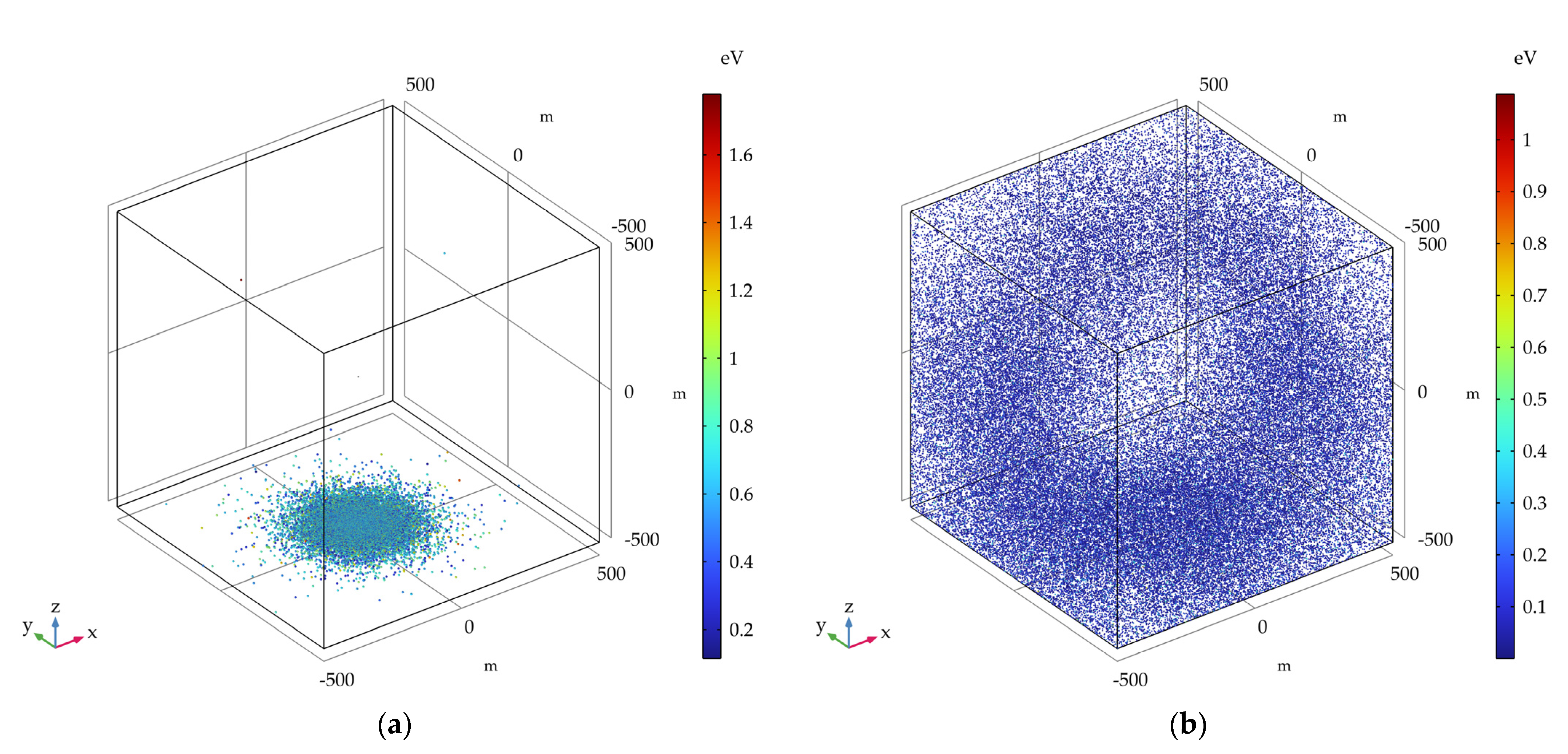
The simulation results of the influence of surface material outgassing on detection for different solar activities, geomagnetic activities, and altitudes were zero for all cases, except for the MM case, where there was a transmission probability of 0.0011% at 280 km. The simulation results in the MM case at 120 km and 320 km are shown in Figure 6. According to the simulation results and Table 5, it can be estimated that the number of outgassing particles entering the sampling port at 280 km in the MM case can reach 1.11 × 10¹³. According to the sampling port area, rocket speed, simulation time, and numerical density of various molecules in the background atmosphere, it can be calculated that the number of atmospheric particles entering the sampling port at 280 km in the MM case is 8.45 × 10¹⁴. Combining the simulation results and the above two calculation results, it can be concluded that the influence of surface material outgassing on detection is very small.

3.2. The Influence of Attitude Control Jet on Detection

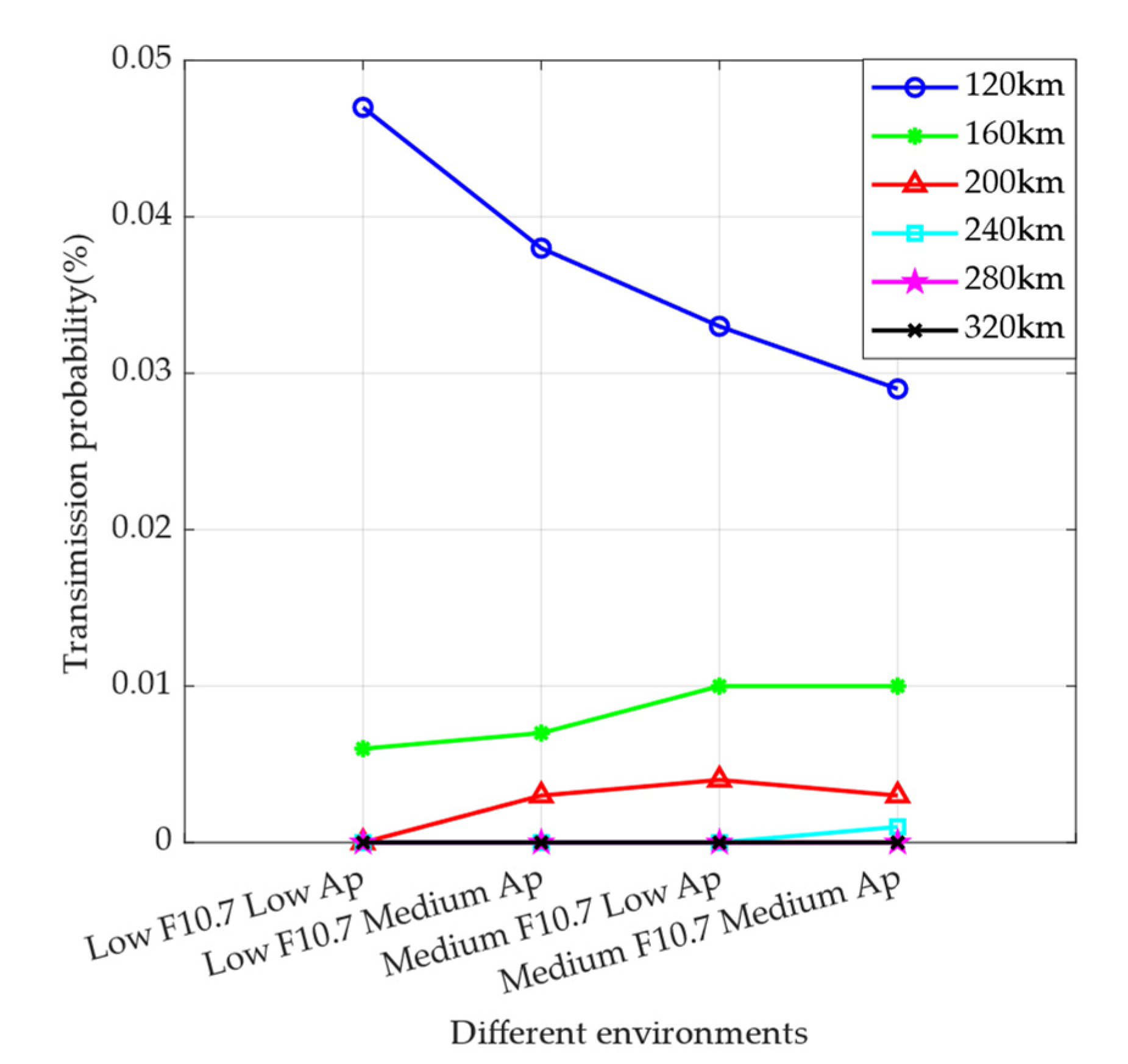
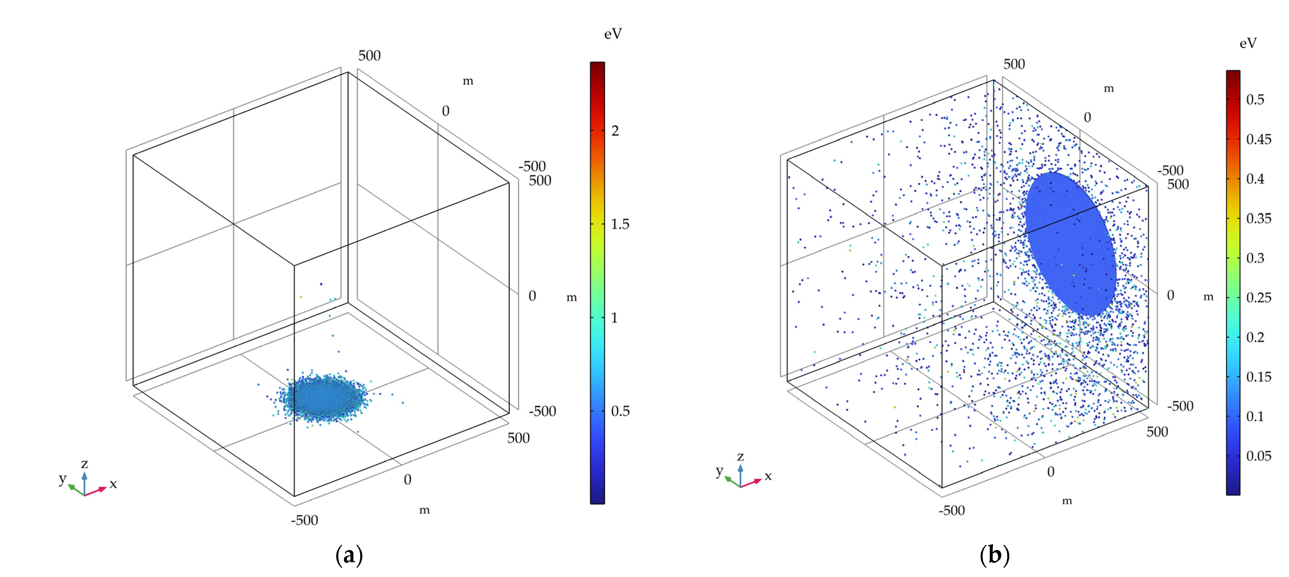
The simulation results of the influence of the attitude control jet on detection for different solar activity, geomagnetic activity, and altitude are shown in

Table 12. Simulation results of the attitude control jet for different solar activities, geomagnetic activities, and altitudes.

Altitude	LL	LM	ML	MM
120 km	0.047%	0.038%	0.033%	0.029%
160 km	0.006%	0.007%	0.010%	0.010%
200 km	0%	0.003%	0.004%	0.003%
240 km	0%	0%	0%	0.001%
280 km	0%	0%	0%	0%
320 km	0%	0%	0%	0%

and Figure 7, and the simulation results in the LL case at 120 km and 320 km are shown in Figure 8. According to the results, it can be observed that the transmission probability gradually decreases at 120 km as the solar activity and geomagnetic activity become intense, while the opposite situation is observed at 160 km, 200 km, and 240 km, where the transmission probability increases as the solar activity and geomagnetic activity become intense; above 240 km, the transmission probability is 0 and there is no trend.

From Table 4, Table 5, Table 6 and Table 7, it can be seen that the numerical density decreases as altitude increases. Additionally, the molecules’ average speed in the background atmosphere increases as temperature increases. However, the average collision frequency decreases according to Equation (3). Therefore, the lower the altitude, the more intense the collision. At the same altitude, the temperature increases due to intense solar activity or geomagnetic activity, and the numerical density of the background atmosphere increases; thus, the average collision frequency increases. The transmission probability decreases as the average collision frequency increases because the background atmosphere is dense and collisions are intense at 120 km, while the transmission probability increases as the average collision frequency increases because the background atmosphere is thin at 160 km, 200 km, and 240 km. Above 240 km, the background atmosphere is very thin, the average collision frequency is less than 1 Hz, and the transmission probability decreases to 0.

Based on the storage conditions of the gas used for attitude control in the mission, with a pressure of 42 MPa, a temperature of 303 K, and a volume of 6 dm³, the number of gas molecules used for attitude control was calculated to be 6.77 × 10²⁵. Based on the sampling port area, the average speed of the platform, the overall flight time, and the numerical density of various molecules in the background atmosphere, the number of atmospheric particles entering the sampling port was calculated to be 1.53 × 10¹⁸. Combining Table 12 with the above two calculation results, it was necessary to reduce the attitude control at low altitudes and decrease the transmission probability. Therefore, the jet-related parameters were optimized to decrease the transmission probability.

3.3. The Influence of Nozzle Outlet Cross-Sectional Area on Detection

3.3.1. N₂

According to the principle of the de Laval nozzle, changing the jet speed must change the outlet cross-sectional area of the nozzle. According to Equations (4) and (5), the speed of sound can be calculated to be about 355 m/s, and the maximum speed can reach 869 m/s after the acceleration of the de Laval nozzle.

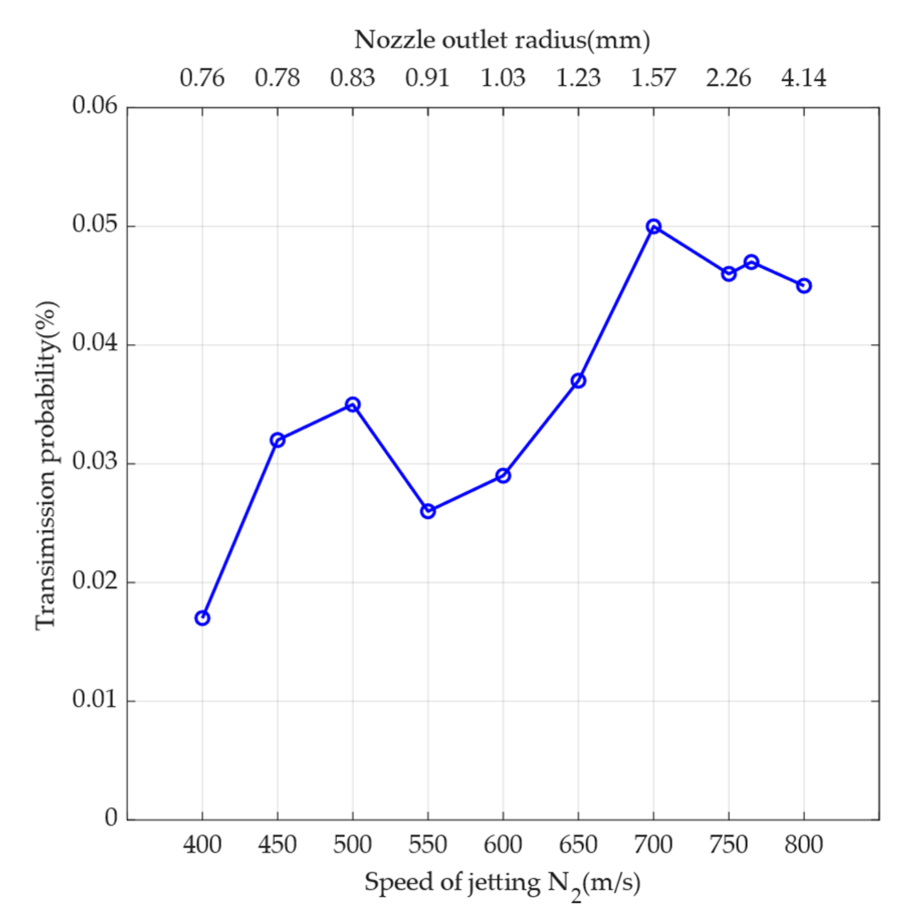
After fixing other parameters and changing the jet speed to 120 km in the LL case, the simulation results are shown in Figure 9. According to Figure 9, it can be observed that the transmission probability shows an overall increasing trend as the speed increases. However, there is a local decrease after 500 m/s and 700 m/s, respectively. From Figure 9, the transmission probability can be reduced by increasing the jet speed to 800 m/s, i.e., by increasing the nozzle outlet cross-sectional area to a radius of 4.14 mm. This can also increase the thrust at the same time to reduce the jet time.

3.3.2. He

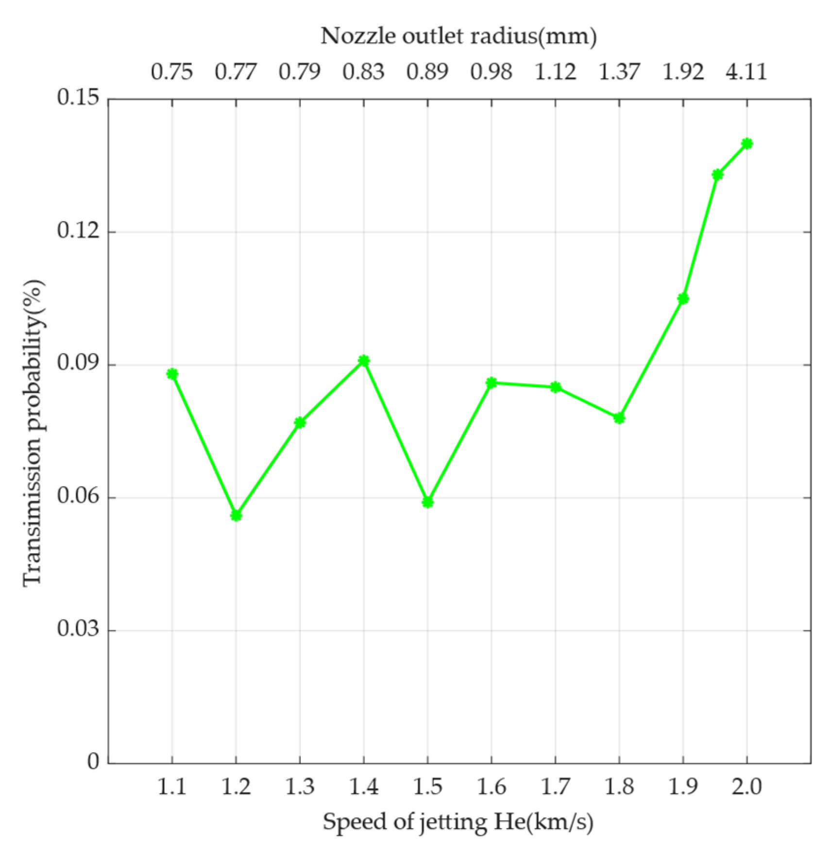
The inert gases N₂ or He are usually chosen as the working gas for cold gas propulsion. If the working gas is changed to He, the speed of sound is about 1022 m/s, and the maximum speed can reach 2051 m/s after acceleration by the de Laval nozzle. The simulation results are shown in Figure 10 for this situation. According to Figure 10, the transmission probability tends to oscillate and then increase as the speed increases; the transmission probability oscillates between 1100 and 1800 m/s and increases after 1800 m/s; the transmission probability of jetting He is higher than the transmission probability of jetting N₂ as a whole. Therefore, N₂ is more suitable for jetting.

3.3.3. N₂ Temperature

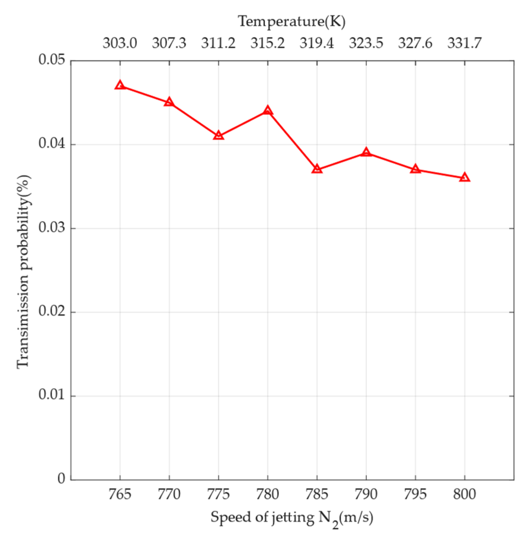
According to Equation (4), if the speed of sound is changed, the speed of jetting can be changed while the outlet cross-sectional area remains unchanged. Based on Equations (4) and (5), if the temperature of the gas is increased to 333 K, the mission design of 765 m/s can be increased to 801 m/s. The simulation results for this situation are shown in Figure 11. According to Figure 11, the jet speed increases with increasing temperature, and the overall transmission probability tends to decrease. Therefore, the temperature of the gas can be increased based on engineering needs.

3.4. The Influence of Nozzle Rotation Angle and Outlet Angle on Detection

3.4.1. Rotation Angle

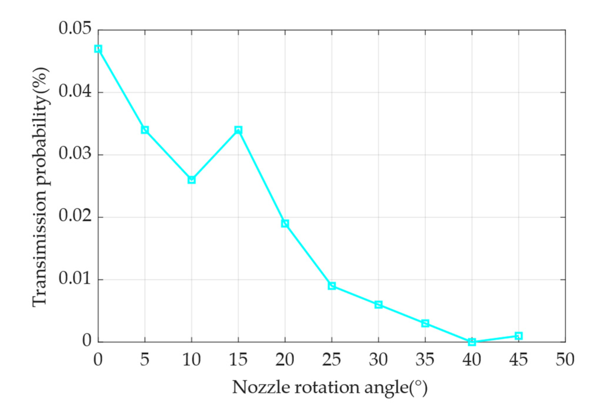
After fixing other parameters and increasing the nozzle rotation angle in the LL case to 120 km, the simulation results are shown in Figure 12. According to Figure 12, the larger the nozzle rotation angle, the smaller the transmission probability. When the nozzle rotation angle is greater than 25°, the transmission probability decreases by an order of magnitude. Additionally, when the nozzle rotation angle increases by more than 40°, the transmission probability basically decreases to zero. From Figure 12, it can be concluded that increasing the nozzle rotation angle can effectively reduce the transmission probability.

3.4.2. Outlet Angle

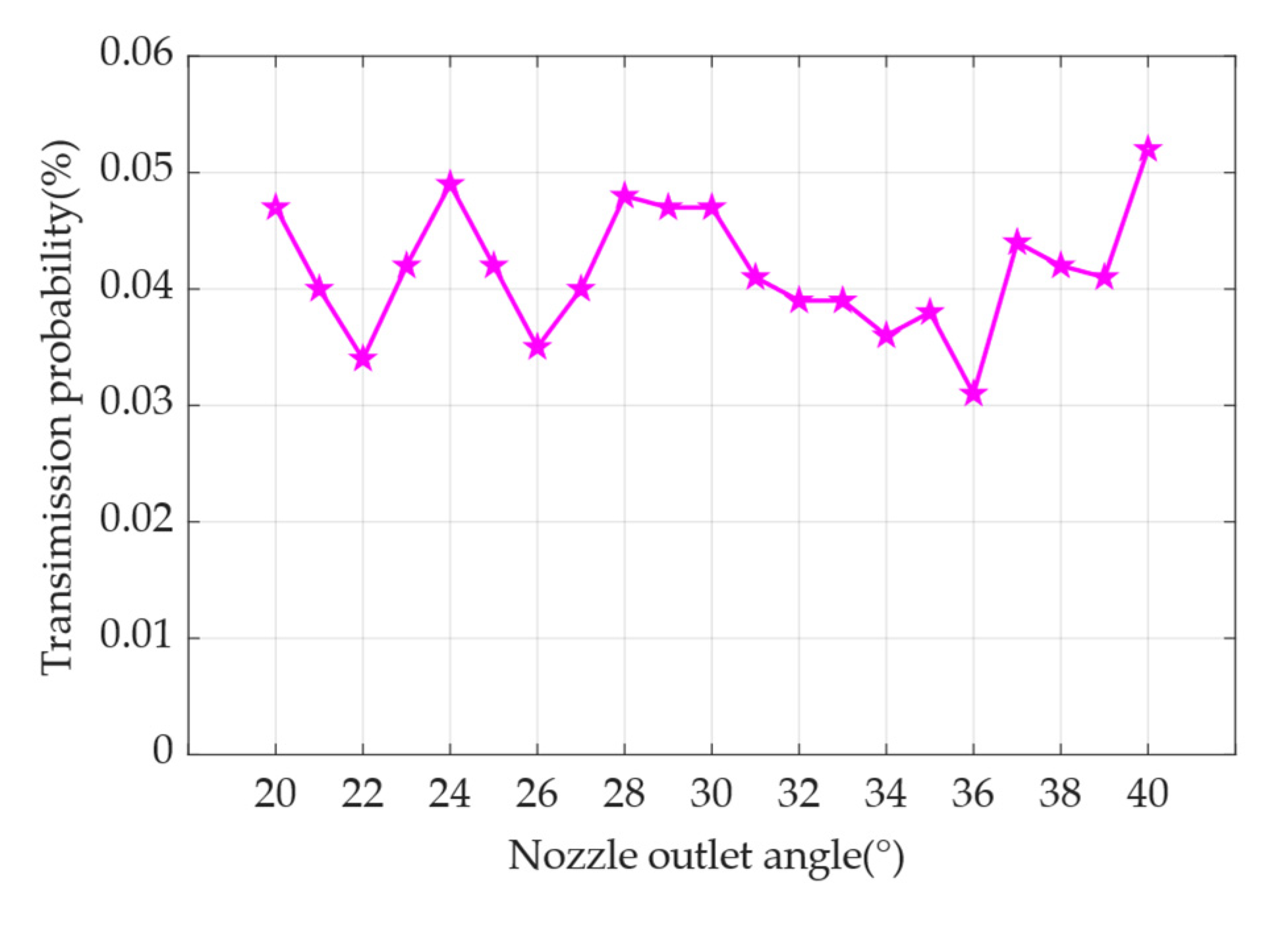
The simulation results are shown in Figure 13, with the other parameters fixed at 120 km in the LL case. According to Figure 13, the transmission probability oscillates as the outlet angle increases. The minimum transmission probability is 0.034% for 22°, and the maximum transmission probability is 0.052% for 40°. From Figure 13, the outlet angle can be increased in the range of 30° to 36°.

3.5. The Influence of Nozzle Center Height on Detection

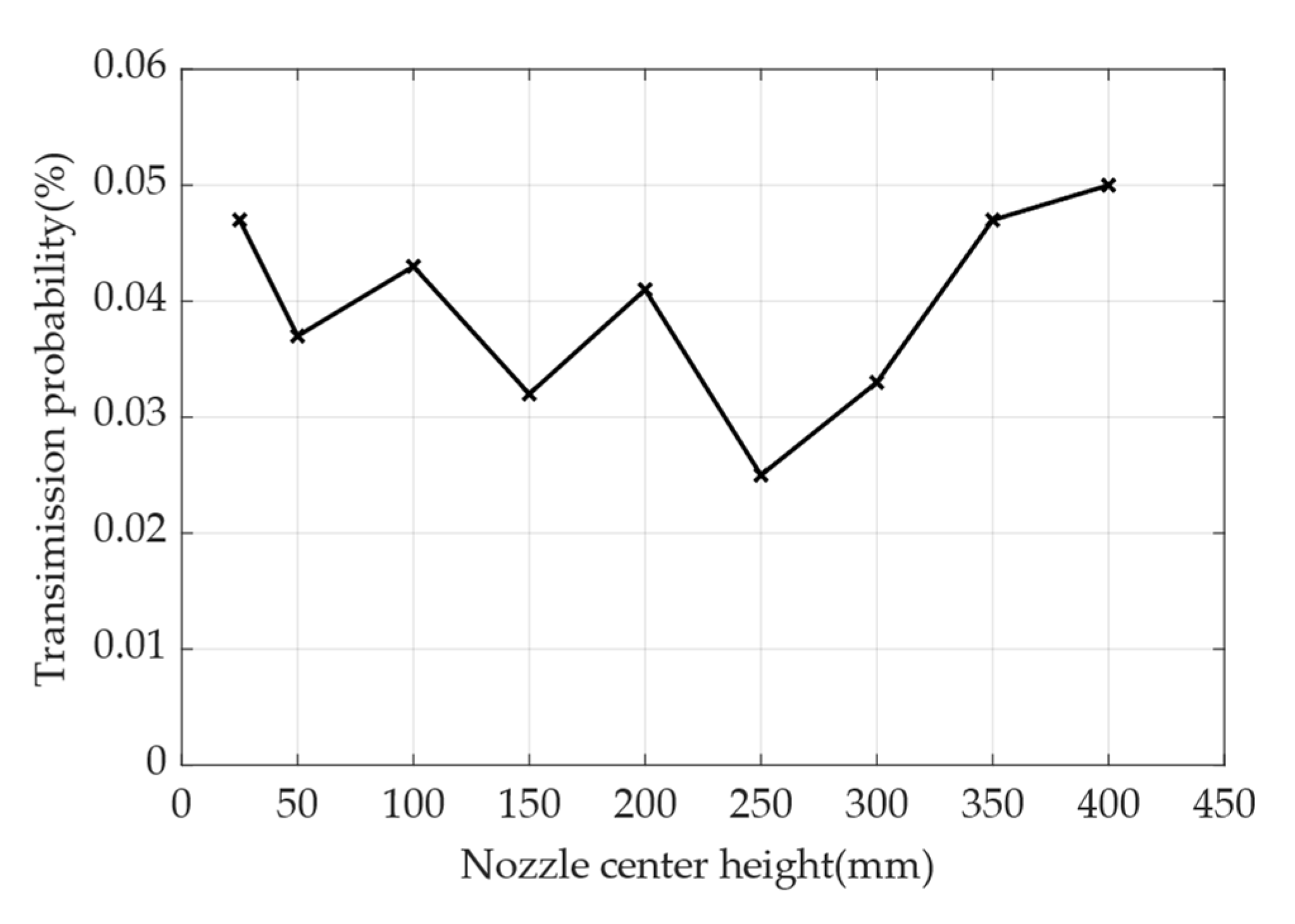
After fixing other parameters and changing the center height of the nozzle, the simulation results are shown in Figure 14. From Figure 14, it can be seen that the transmission probability with the increase of center height decreases and then increases. The decreasing interval shows oscillating falls, and the minimum transmission probability is 0.025% at 250 mm. Then, in increasing intervals, there is a maximum transmission probability of 0.050% at 400 mm. Therefore, the nozzle center height can be increased to a range of less than 250 mm to reduce the probability of transmission.

4. Conclusions

In this paper, the collision process between gas molecules from surface materials outgassing and the attitude control jet with the background atmosphere was modeled, simulated, and analyzed using the physical field simulation software COMSOL and the Monte Carlo method in the context of the Meridian Project sounding rocket mission. Using the model, it can be investigated whether the gas molecules of two cases can enter the sampling port of the mass spectrometer sensor for in-situ atmospheric detection, and the methods to reduce the transmission probability can be investigated by simulating and optimizing the parameters related to the jet and obtaining the following conclusions:

• A simulation model based on COMSOL and Monte Carlo was proposed to simulate and analyze the influence of surface material outgassing and attitude control jet on sounding rocket detection under different solar activity, geomagnetic activity, and altitude;
• Regardless of medium or low solar activity or medium or low geomagnetic activity, surface material outgassing has little influence on sounding rocket detection. However, a low-altitude attitude control jet has a greater influence on sounding rocket detection, which can be reduced by reducing the number of low-altitude attitude controls and decreasing the transmission probability;
• According to the simulation, the transmission probability can be reduced by increasing the cross-sectional area of the de Laval nozzle outlet or increasing the gas temperature for attitude control within the allowable range of the project. Increasing the nozzle’s rotation angle, the outlet angle within 36°, and the center height within 250 mm can decrease the transmission probability;
• Since the NRLMSISE-00 model is higher than the actual atmospheric measurement data, the actual transmission probability should be lower than the calculation results of the simulation.

References

- European Space Agency. Erasmus Experiment Archive. Available online: https://eea.spaceflight.esa.int/portal/?plid=4 (accessed on 1 March 2023).
- European Space Agency. ESA—Search. Available online: https://www.esa.int/esearch?q=sounding+rocket (accessed on 6 March 2023).
- Seibert, G. The History of Sounding Rockets and Their Contribution to European Space Research; ESA Publications Division: Noordwijk, The Netherlands, 2006. [Google Scholar]
- Wade, M. R-1. Available online: http://astronautix.com/r/r-1.html (accessed on 2 March 2023).
- Krebs, G.D. R-11A. Available online: https://space.skyrocket.de/doc_lau/r-11a.htm (accessed on 7 March 2023).
- Adkins, J. Sounding Rockets. Available online: http://www.nasa.gov/mission_pages/sounding-rockets/index.html (accessed on 1 March 2023).
- Japan Aerospace Exploration Agency. Sounding Rockets—ISAS. Available online: https://www.isas.jaxa.jp/en/missions/sounding_rockets/ (accessed on 1 March 2023).
- Suresh, B.N. History of Indian Launchers. Acta Astronaut. 2008, 63, 428–434. [Google Scholar] [CrossRef]
- Pandey, K.; Gupta, S.P. Altitude of Two-Stream Irregularities in Equatorial E Region Using Sounding Rocket Experiments from Thumba. J. Geophys. Res. Space Phys. 2020, 125, e2019JA027195. [Google Scholar] [CrossRef]
- Abe, T.; Kurihara, J.; Iwagami, N.; Nozawa, S.; Ogawa, Y.; Fujii, R.; Hayakawa, H.; Oyama, K. Dynamics and Energetics of the Lower Thermosphere in Aurora (DELTA)—Japanese Sounding Rocket Campaign. Earth Planets Space 2006, 58, 1165–1171. [Google Scholar] [CrossRef] [Green Version]
- Lyubimova, T.; Ivantsov, A.; Garrabos, Y.; Lecoutre, C.; Beysens, D. Faraday Waves on Band Pattern under Zero Gravity Conditions. Phys. Rev. Fluids 2019, 4, 064001. [Google Scholar] [CrossRef]
- Chernyshov, A.A.; Spicher, A.; Ilyasov, A.A.; Miloch, W.J.; Clausen, L.B.N.; Saito, Y.; Jin, Y.; Moen, J.I. Studies of Small-Scale Plasma Inhomogeneities in the Cusp Ionosphere Using Sounding Rocket Data. Phys. Plasmas 2018, 25, 042902. [Google Scholar] [CrossRef] [Green Version]
- Moshkov, A.V.; Pozhidaev, V.N. Vertical Distribution of a Demodulated Low-Frequency Field in the Disturbed Low-Latitude Ionosphere. J. Commun. Technol. Electron. 2018, 63, 118–122. [Google Scholar] [CrossRef]
- Li, D. Development of The Third Generation Sounding Rockets of China. Spacecr. Recovery Remote Sens. 1997, 18, 46–58. [Google Scholar]
- Jiang, X.; Liu, B.; Yu, S.; Chen, P.; Shi, H. Development Status and Trend of Sounding Rocket. Sci. Technol. Rev. 2009, 27, 101–110. [Google Scholar]
- Wang, C. New Chains of Space Weather Monitoring Stations in China. Space Weather 2010, 8, 1–5. [Google Scholar] [CrossRef]
- Wang, C.; Xu, J.; Lü, D.; Yue, X.; Xue, X.; Chen, G.; Yan, J.; Yan, Y.; Lan, A.; Wang, J.; et al. Construction Progress of Chinese Meridian Project Phase II. Chin. J. Space Sci. 2022, 42, 539–545. [Google Scholar] [CrossRef]
- Liu, W.; Michel, B.; Wang, C.; Xu, J.; Li, H.; Ren, L.; Liu, Z.; Zhu, Y.; Li, G.; Li, L.; et al. Progress of International Meridian Circle Program. Chin. J. Space Sci. 2022, 42, 584–587. [Google Scholar] [CrossRef]
- Wang, C.; Ren, L. Recent Development and Preliminary Results of Chinese Meridian Project. Chin. J. Space Sci. 2013, 33, 1–5. [Google Scholar] [CrossRef]
- Wang, C.; Wang, J.; Xu, J. Research Advances of the Chinese Meridian Project in 2020–2021. Chin. J. Space Sci. 2022, 42, 574–583. [Google Scholar] [CrossRef]
- Khamees, H.T. Average Intensity of SLVGB for Slant Path Propagation in Atmospheric Turbulent. Results Opt. 2021, 5, 100159. [Google Scholar] [CrossRef]
- Khamees, H.T. Laser Gaussian Beam Analysis of Structure Constant Depends on Kolmogorov in Turbulent Atmosphere for a Variable Angle of Wave Propagation. J. Laser Appl. 2022, 34, 022017. [Google Scholar] [CrossRef]
- Ketsdever, A.D.; Gimelshein, S. A Spacecraft’s Own Ambient Environment: The Role of Simulation-Based Research. In Proceedings of the 29th International Symposium on Rarefied Gas Dynamics, Xi’an, China, 13 July 2014; pp. 1394–1401. [Google Scholar]
- Justiz, C.R.; Sega, R.M.; Dalton, C.; Ignatiev, A. DSMC- and BGK-Based Calculations for Return Flux Contamination of an Outgassing Spacecraft. J. Thermophys. Heat Transf. 1994, 8, 802–803. [Google Scholar] [CrossRef]
- Manning, H.L.K.; Frank, N.J.; Bursack, J.; Johnson, B.W.; Benner, S.M.; Chen, P.T.C. Return Flux Experiment; REFLEX: Spacecraft Self-Contamination. In Proceedings of the Optical System Contamination: Effects, Measurements, and Control VII, Seattle, WA, USA, 9 July 2002; pp. 184–198. [Google Scholar]
- Soares, C.E.; Mikatarian, R.R. Mir Contamination Observations and Implications to the International Space Station. In Proceedings of the Optical Systems Contamination and Degradation II: Effects, Measurements, and Control, San Diego, CA, USA, 2 August 2000; pp. 55–65. [Google Scholar]
- Hässig, M. Investigation of Spacecraft Outgassing by Sensitive Mass Spectrometry. Spectrosc. Eur. 2011, 23, 20–23. [Google Scholar]
- Isobe, N.; Nakagawa, T.; Okazaki, S.; Sato, Y.; Ando, M.; Baba, S.; Miura, Y.; Miyazaki, E.; Kimoto, Y.; Ishizawa, J.; et al. Contamination Control for the Space Infrared Observatory SPICA. In Proceedings of the Space Telescopes and Instrumentation 2014: Optical, Infrared, and Millimeter Wave, Montréal, QC, Canada, 22 June 2014; pp. 1–11. [Google Scholar]
- Altwegg, K.; Balsiger, H.; Calmonte, U.; Hässig, M.; Hofer, L.; Jäckel, A.; Schläppi, B.; Wurz, P.; Berthelier, J.J.; De Keyser, J.; et al. In Situ Mass Spectrometry during the Lutetia Flyby. Planet. Space Sci. 2012, 66, 173–178. [Google Scholar] [CrossRef]
- Xie, L.; Zhang, X.; Zheng, Y.; Guo, D. The Effects of Spacecraft Charging and Outgassing on the LADEE Ion Measurements. J. Geophys. Res. Space Phys. 2017, 122, 5825–5834. [Google Scholar] [CrossRef]
- Schläppi, B.; Altwegg, K.; Balsiger, H.; Hässig, M.; Jäckel, A.; Wurz, P.; Fiethe, B.; Rubin, M.; Fuselier, S.A.; Berthelier, J.J.; et al. Influence of Spacecraft Outgassing on the Exploration of Tenuous Atmospheres with in Situ Mass Spectrometry. J. Geophys. Res. Space Phys. 2010, 115, 1–14. [Google Scholar] [CrossRef]
- Bird, G.A. Monte Carlo Simulation of Gas Flows. Annu. Rev. Fluid Mech. 1978, 10, 11–31. [Google Scholar] [CrossRef]
- Hall, D.F.; Arnold, G.S.; Simpson, T.R.; Suess, D.R.; Nystrom, P.A. Progresson Spacecraft Contamination Model Development. In Proceedings of the Optical Systems Contamination and Degradation II: Effects, Measurements, and Control, San Diego, CA, USA, 2 August 2000; pp. 138–156. [Google Scholar]
- Brieda, L. Molecular Contamination Modeling with CTSP. In Proceedings of the 30th International Symposium on Rarefied Gas Dynamics, Victoria, BC, Canada, 10 July 2016; pp. 1–8. [Google Scholar]
- Chang, C.W.; Kannenberg, K.; Chidester, M.H. Development of Versatile Molecular Transport Model for Modeling Spacecraft Contamination. In Proceedings of the Optical System Contamination: Effects, Measurements, and Control 2010 (SPIE), San Diego, CA, USA, 2 August 2010; pp. 1–8. [Google Scholar]
- Kimoto, Y. Contamination Control Research Activities for Space Optics in JAXA R&D. In Proceedings of the International Conference on Space Optics—ICSO 2014 (SPIE), Tenerife, Spain, 7 October 2014; pp. 1–6. [Google Scholar]
- Dirri, F.; Palomba, E.; Longobardo, A.; Zampetti, E.; Saggin, B.; Scaccabarozzi, D. A Review of Quartz Crystal Microbalances for Space Applications. Sens. Actuators Phys. 2019, 287, 48–75. [Google Scholar] [CrossRef]
- Abraham, N.S.; Hasegawa, M.M.; Straka, S.A. Development and Testing of Molecular Adsorber Coatings. In Proceedings of the Optical System Contamination: Effects, Measurements, and Control 2012, San Diego, CA, USA, 13 August 2012; Volume 8492, pp. 1–11. [Google Scholar]
- Faye, D.; Jakob, A.; Soulard, M.; Berlioz, P. Zeolite Adsorbers for Molecular Contamination Control in Spacecraft. In Proceedings of the Optical System Contamination: Effects, Measurements, and Control 2010, San Diego, CA, USA, 2 August 2010; pp. 1–14. [Google Scholar]
- Tseng, W.-L.; Lai, I.-L.; Ip, W.-H.; Hsu, H.-W.; Wu, J.-S. The 3D Direct Simulation Monte Carlo Study of Europa’s Gas Plume. Universe 2022, 8, 261. [Google Scholar] [CrossRef]
- Marschall, R.; Su, C.C.; Liao, Y.; Thomas, N.; Altwegg, K.; Sierks, H.; Ip, W.-H.; Keller, H.U.; Knollenberg, J.; Kührt, E.; et al. Modelling Observations of the Inner Gas and Dust Coma of Comet 67P/Churyumov-Gerasimenko Using ROSINA/COPS and OSIRIS Data: First Results. Astron. Astrophys. 2016, 589, A90. [Google Scholar] [CrossRef]
- Picone, J.M.; Hedin, A.E.; Drob, D.P.; Aikin, A.C. NRLMSISE-00 Empirical Model of the Atmosphere: Statistical Comparisons and Scientific Issues. J. Geophys. Res. Space Phys. 2002, 107, 1–16. [Google Scholar] [CrossRef]
- Emmert, J.T. Thermospheric Mass Density: A Review. Adv. Space Res. 2015, 56, 773–824. [Google Scholar] [CrossRef]
- Chen, M.; Xue, S.; Zhou, Z.; Liu, J.; Li, B. Outgassing Performance Research on CuCrZr. Chin. J. Vac. Sci. Technol. 2021, 41, 766–769. [Google Scholar] [CrossRef]
- Patrick, T.J. Outgassing and the Choice of Materials for Space Instrumentation. Vacuum 1973, 23, 411–413. [Google Scholar] [CrossRef]
- COMSOL Inc. COMSOL: Multiphysics Software for Optimizing Designs. Available online: https://www.comsol.com/ (accessed on 2 March 2023).
- Wong, C.M.; Moision, R.M.; Fowler, J.D.; Liu, D.L. Molecular Transport Modeling for Spaceborne Instrument Contamination Prediction. In Proceedings of the Systems Contamination—Prediction, Measurement, and Control 2014, San Diego, CA, USA, 18 August 2014; pp. 1–12. [Google Scholar]
- Qiao, J.; Yang, S.; Li, J.; Guo, X.; Wang, Y. Dynamic Simulation of Deposition Processes of Spacecraft Molecular Contamination. Teh. Vjesn.-Tech. Gaz. 2021, 28, 321–327. [Google Scholar] [CrossRef]
- Wong, C.M.; Labatete-Goeppinger, A.C.; Fowler, J.D.; Easton, M.P.; Liu, D.L. Outgassing Study of Spacecraft Materials and Contaminant Transport Simulations. In Proceedings of the Systems Contamination: Prediction, Control, and Performance 2016, San Diego, CA, USA, 31 August 2016; pp. 1–9. [Google Scholar]
- COMSOL Inc. COMSOL Help Desk. Available online: https://doc.comsol.com/6.1/docserver/VAADIN/themes/docserver/_self/helpdesk/helpdesk.html (accessed on 4 March 2023).
Figure 1.
Diagram of the incident molecular motion.
Figure 2.
Structure of the de Laval nozzle. The three straight arrows are the inlet, throat and outlet from left to right, where A* is the cross-sectional area of throat and the speed is 1 Ma at this point. The only curved arrow indicates the outlet angle θ.
Figure 3.
Relationship between Ma and A*/A(x). The x-axis represents the Mach number, which is the ratio of the jet speed to the local speed of sound (the blue line intersects the x-axis at , and the green line intersects the x-axis at ). The y-axis represents the ratio of the cross-sectional area of the throat to any cross-sectional area of the nozzle.
Figure 4.
Flowchart of building model.
Figure 5.
Structure of the model: (a) the sounding rocket platform; (b) the sensor sampling port of the mass spectrometer for in-situ atmospheric detection; (c) the outlet of the de Laval nozzle for the attitude control jet, which is the blue area; and (d) the collision domain used to simulate the collision process.
Figure 6.
Simulation results of surface material outgassing in the MM case: (a) 120 km; (b) 320 km.
Figure 7.
Simulation results of the attitude control jet under different environments. The x-axis represents the gradual intensification of solar activity and geomagnetic activity, where F10.7 represents the degree of solar activity and Ap represents the degree of geomagnetic activity. The y-axis represents the transmission probability, which is the ratio of the number of particles received at the sensor sampling port to the total number of particles.
Figure 8.
Simulation results of the attitude control jet in the LL case: (a) 120 km; (b) 320 km.
Figure 9.
Relationship between the speed of jetting N2 and transmission probability. The simulation results are indicated by circles in the line graph. The primary x-axis at the bottom indicates the speed of jetting N2, and the secondary x-axis at the top indicates the nozzle outlet radius at the corresponding speed. The y-axis indicates the transmission probability, which is the ratio of the number of particles received at the sensor sampling port to the total number of particles.
Figure 10.
Relationship between the speed of jetting He and transmission probability. The simulation results are indicated by stars in the line graph. The primary x-axis at the bottom indicates the speed of jetting He, and the secondary x-axis at the top indicates the nozzle outlet radius at the corresponding speed. The y-axis indicates the transmission probability, which is the ratio of the number of particles received at the sensor sampling port to the total number of particles.
Figure 11.
Relationship between speed of jetting N2 and transmission probability. The simulation results are indicated by triangles in the line graph. The primary x-axis at the bottom indicates the speed of jetting N2, and the secondary x-axis at the top indicates the temperature at the corresponding speed. The y-axis indicates the transmission probability, which is the ratio of the number of particles received at the sensor sampling port to the total number of particles.
Figure 12.
Relationship between nozzle rotation angle and transmission probability. The simulation results are indicated by squares in the line graph. The x-axis represents the nozzle rotation angle, which is the angle between the outer normal vector of the nozzle outlet and the x-axis in Figure 5. The y-axis represents the transmission probability, which is the ratio of the number of particles received at the sensor sampling port to the total number of particles.
Figure 13.
Relationship between nozzle outlet angle and transmission probability. The simulation results are indicated by pentagrams in the line graph. The x-axis represents the nozzle outlet angle, as shown in Figure 2 and Table 1. The y-axis represents the transmission probability, which is the ratio of the number of particles received at the sensor sampling port to the total number of particles.
Figure 14.
Relationship between nozzle center height and transmission probability. The simulation results are indicated by x-marks in the line graph. The x-axis represents the nozzle center height, as shown in Figure 5c, which is the location of the nozzle. The y-axis represents the transmission probability, which is the ratio of the number of particles received at the sensor sampling port to the total number of particles.