Article

Temporal Variation of NO2 and O3 in Rome (Italy) from Pandora and In Situ Measurements

by
Annalisa Di Bernardino
1,*,
Gabriele Mevi
2,
Anna Maria Iannarelli
2,
Serena Falasca
1,
Alexander Cede
3,
Martin Tiefengraber
3 and
Stefano Casadio
2,4
1
Physics Department, Sapienza University of Rome, 00185 Rome, Italy
2
SERCO Italia SpA, Frascati, 00044 Rome, Italy
3
LuftBlick, 6020 Innsbruck, Austria
4
ESA-ESRIN, 00044 Frascati, Italy
*
Author to whom correspondence should be addressed.
Atmosphere 2023, 14(3), 594; https://doi.org/10.3390/atmos14030594
Submission received: 20 February 2023 / Revised: 15 March 2023 / Accepted: 17 March 2023 / Published: 21 March 2023

Abstract

:
To assess the best measures for the improvement of air quality, it is crucial to investigate in situ and columnar pollution levels. In this study, ground-based measurements of nitrogen dioxide (NO2) and ozone (O3) collected in Rome (Italy) between 2017 and 2022 are analyzed. Pandora sun-spectrometers provided the time series of the NO2 vertical column density (VC-NO2), tropospheric column density (TC-NO2), near-surface concentration (SC-NO2), and the O3 vertical column density (VC-O3). In situ concentrations of NO2 and O3 are provided by an urban background air quality station. The results show a clear reduction of NO2 over the years, thanks to the recent ecological transition policies, with marked seasonal variability, observable both by columnar and in situ data. Otherwise, O3 does not show inter-annual variations, although a clear seasonal cycle is detectable. The results suggest that the variation of in situ O3 is mainly imputable to photochemical reactions while, in the VC-O3, it is triggered by the predominant contribution of stratospheric O3. The outcomes highlight the importance of co-located in situ and columnar measurements in urban environments to investigate physical and chemical processes driving air pollution and to design tailored climate change adaptation strategies.

1. Introduction

The World Health Organization (WHO) estimates that seven million people yearly die prematurely because of air pollution worldwide [1] and, despite the interest of the scientific community and technological advancement of recent years, nine out of ten people breathe air that exceeds the limits of outdoor pollutants provided by WHO [2].
Several studies have demonstrated that atmospheric pollution affects medium and small-sized cities [3,4], even if the problem is more evident in large urban areas and metropolises [5,6], where the uneven distribution of emissive sources, the complex arrangement of buildings, and the composite photochemical reactions seriously complicate the assessment of the air quality level [7]. Moreover, the dense geometry of buildings and streets reduces the ventilation at the pedestrian level, limiting the exchange of momentum and mass between the canyons and the free atmosphere, further worsening the air quality and, consequently, the urban livability and human comfort [8,9].
To improve ambient air quality and tackle atmospheric pollution, during the last few decades international government bodies have promulgated numerous regulations. Specifically, in Europe, the European Directive 1999/30/EC [10] and, more recently, the European Air Quality Directive 2008/50/EC [11] have established outdoor air quality standards for key pollutants. Regulated and monitored harmful atmospheric substances include nitrogen oxides (NOx), nitrogen dioxide (NO2), ozone (O3), sulfur dioxide (SO2), benzene (C6H6), carbon monoxide (CO), and particulate matter (PM). Among these, NO2 and O3 are recognized among the compounds most capable of producing adverse impacts on human health and ecosystems [12,13,14].
NO2 is chiefly emitted from the combustion of fossil fuels at high temperatures (as in motor vehicles), along with the combustion of natural sources (such as forest fires and volcanos). Moreover, it is produced as a secondary pollutant by the reaction of NO with excess oxygen, in turn generated by the oxidative decomposition of ammonia. It has a relatively short photochemical lifetime, ranging between 2 and 6 h during sunny summer days [15] and between 12 and 24 h in winter [16]. The seasonal variation of NO2 in the atmosphere is also strongly influenced by the meteorological conditions and by the solar zenith angle (SZA), which determines the solar radiation intensity. Nonetheless, thanks to the photochemical reactions occurring in the atmosphere and the short lifetime of NO2, its tropospheric concentration can be assumed closely related to local traffic sources. In fact, according to the report of Air Quality Europe 2022 [17], in Europe, road traffic contributes to about 37% of the total NO2 emissions. Moreover, the tropospheric reactions involving NO2 lead to the formation of strong oxidants, responsible for the conversion of NO2 to nitric acid and SO2. The latter substances are important sources of organic, nitrate, and sulphate particles, and contribute to the increase of atmospheric PMs.
Ozone is a reactive gas present in two layers of the atmosphere: the stratosphere and the troposphere. The stratospheric ozone protects the Earth from the Sun’s harmful ultraviolet radiation. Unlike the stratospheric O3, the ground-level (or tropospheric) ozone is a greenhouse gas causing adverse effects on human health and ecosystems. In urban areas, the concurrent presence of high levels of NOx and Volatile Organic Compounds (VOCs), which are the chemical precursors of O3, can give rise to the photolysis reactions of NO2 into NO and oxygen radicals [18,19]. The latter reacts with atmospheric oxygen molecules generating O3. It follows that the formation of tropospheric ozone is driven by the absolute concentrations of NOx and VOCs, the ratio between the latter two substances, the intensity of incoming solar radiation, and the air temperature, resulting in a clear diurnal and seasonal pattern. As an example, Lal and Subbaraya [20] showed that in Delhi (India) the O3 concentration starts increasing gradually after sunrise, attains maximum value during noontime, and then decreases, assuming minima during early morning hours. They observed the maximum O3 values during spring/summer due to the large availability of solar radiation. Moreover, due to the well-known chemical coupling of O3 and NOx, O3 and NO2 levels are inextricably linked by complex non-linear chemical reactions and are typically studied in conjunction. For instance, Karl et al. [19] focused on the O3-NO-NO2 triad, revealing that the downward flux of ozone is primarily due to the rapid conversion of NO to NO2, while Han et al. [21] studied the relationship between O3, NO, and NO2 in China finding a diurnal cycle of ground-level O3 with a mid-day peak and lower nighttime concentrations and highlighting a linear relationship between NO2 and NOx, as well as NO and NOx, and a polynomial relationship between O3 and NO2/NO.
The amount of trace gases in the atmosphere can be investigated through several in situ and remote sensing techniques. For instance, satellite remote sensing measurements allow the investigation of atmospheric chemical composition worldwide, also covering oceans and remote areas, but their spatial resolution is often too low to appreciate the heterogeneity of pollution in cities. Furthermore, the largest amount of tropospheric NO2 is typically located in the boundary layer close to the emission sources, i.e., in the atmospheric layer most difficult to reach through satellite measurements. It follows that ground-based remote sensing measurements are fundamental both to support the validation of satellite products and to retrieve columnar and surface amounts of trace gases. Moreover, for a comprehensive study of air quality, it is necessary to synergistically integrate satellite and columnar observations with in situ measurements, which allow the evaluation of the direct exposure of the population and therefore the impact of pollution on human health and society [22].
The Pandora sun–moon–sky spectrometer, developed by SciGlob Instruments and Services LLC [23], is among the state-of-the-art instruments for the monitoring of atmospheric trace gases [24]. It allows the high temporal resolution retrieval of total vertical column density (VC), tropospheric column density (TC), and near-surface concentration (SC) of several gases, such as NO2 and O3. The Pandonia Global Network (PGN) [25] is a joint activity between the European Space Agency and the National Aeronautics and Space Administration, aiming at providing the scientific community with real-time, standardized, calibrated, and verified air quality data and associated uncertainty values retrieved from Pandora instruments operating worldwide. Pandora measurements have been widely used for satellite data validation [26,27], for inter-comparison with other ground-based instruments [28,29], and for the investigation of spatial and temporal variability of air pollutants [30,31].
In this paper, we analyze the NO2 vertical and tropospheric columnar densities (VC-NO2 and TC-NO2, respectively), NO2 near-surface concentration (SC-NO2), and O3 vertical columnar density (TC-O3) collected by Pandora 2S sun-spectrometers, belonging to PGN, located in the urban area of Rome (Italy). Measurements from 2017 to 2022 are analyzed to (i) compare the columnar and near-surface Pandora measurements with in situ concentrations of NO2 and O3, differentiating weekdays and weekends; (ii) investigate the temporal variability of pollutants and therefore assess the effectiveness of recent emission abatement policies, and (iii) evaluate the variation of the NO2 peak as a function of the month of the year and of the hour of the day to provide useful suggestions to policymakers for the implementation of traffic restrictions during particular time slots.
This paper is structured as follows: Section 2 describes the material and methods, focusing on the description of the observation site, the instruments, the dataset, and the data processing. In Section 3, the main results are presented and discussed, also focusing on the weekday/weekend differences. Finally, the conclusions of the study are drawn in Section 4.

2. Materials and Methods

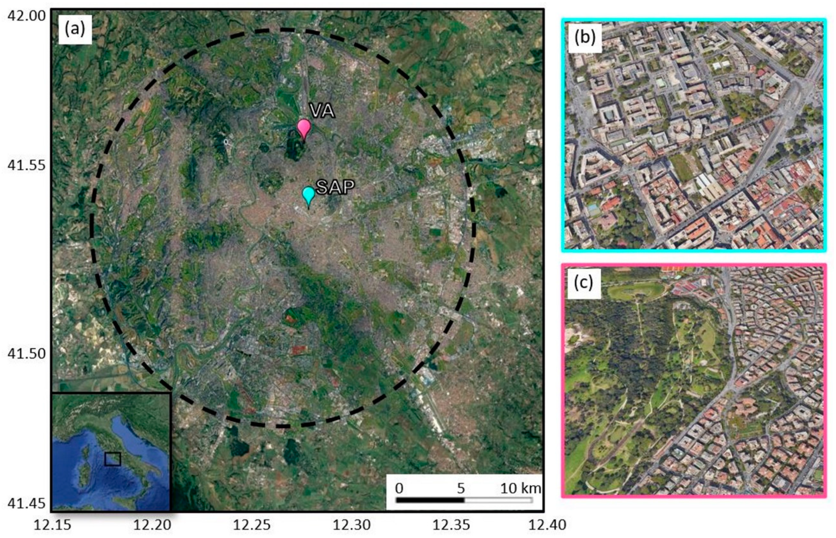
2.1. Description of Observation Site and Instruments

The Metropolitan City of Rome (Lat. 41.91° N, Lon. 12.48° E, Figure 1) has about 2.7 million inhabitants over approximately 1300 km2, resulting in one of the most populated European metropolitan areas. The urban center develops along the Tiber valley, about 27 km inland from the Tyrrhenian coast. Rome belongs to the Csa Köppen–Geiger climate classification, experiencing dry and hot summers and moderate wet and mild winters [32]. From the air quality point of view, the main pollutant sources are vehicular traffic and domestic heating, while the major industrial districts are located south of the city. Moreover, pollution levels are influenced by the two prevailing anemological regimes of the region: the drainage flow through the Tiber valley [33], which can favor the dispersion of the pollutants emitted in the city, and the sea breeze regime [31] that gives rise to Southwest winds during the day carrying clean air from the sea over the center of Rome. Finally, Rome is exposed to the frequent advection of Saharan dust transported through the Mediterranean Sea, responsible for the increase in the in situ and columnar amounts of PM. As highlighted by Ciardini et al. [34], the dust outbreaks follow a seasonal trend, with the maximum occurrence in the period April–June.
The Physics Department of Sapienza University of Rome (hereinafter, SAP), located in a densely built-up district in the center of Rome (Lat. 41.90° N, Lon. 12.51° E, 75 m. a.s.l.) has hosted since 2016 the main observation site of the Boundary-layer Air Quality-analysis Using Network of Instruments (BAQUNIN) atmospheric observatory [35,36]. Since 2017, SAP has hosted the PGN Pandora 2S sun-spectrometers (serial numbers #117 and #138, see Section 2.2). Here, the NO2 and O3 columnar densities and near-surface concentrations are investigated.
Furthermore, to also evaluate the levels of pollution near the ground, hourly in situ concentrations of NO2 and O3 collected at the Villa Ada station (Lat. 41.93° N, Lon. 12.51° E, 50 m. a.s.l., hereinafter, VA) have been considered. VA belongs to the air quality monitoring network managed by the Regional Agency for Environmental Protection (ARPA Lazio) and has been widely used for the investigation of air quality in the center of Rome [37,38,39]. The station is located on the edge of a large park in downtown Rome and therefore is not directly influenced by traffic emissions and could be considered representative of the urban background air quality conditions. The sensors for the measurements of NO2 and O3 (200 E and 400 E, respectively; Teledyne API, San Diego, CA, USA) are checked quarterly, as required by the Italian Legislative Decree 30 March 2017 GU n. 96 [40]. ARPA Lazio provides concentrations in μg/m3 and here values are converted in moles per cubic meter (mol/m3) in order to be compared to near-surface concentrations (for NO2 1 mol/m3 = 2.17 × 10⁻⁴ μg/m3, for O3 1 mol/m3 = 2.08 × 10⁻⁴ μg/m3).
VA is about 3.5 km north of SAP and, as both stations are located in the center of Rome, they can be used to characterize urban pollution levels.

2.2. The Pandora Dataset

The PGN retrieval schemes for NO2, O3, and other trace gases from direct sun measurements, including the so-called Algorithm Theoretical Baseline Document and the guidelines for the correct use of PGN products, are detailed in [41,42]. The radiance spectra underpass several correction/adjustment procedures, such as dark signal, non-linearity, latency, flat field, temperature, sensitivity, and wavelength corrections before the retrieval of geophysical quantities [40]. VC is defined as the total column amount of the studied gas between the altitude of the instrument and the top of the atmosphere. VCs are measured in direct Sun observation mode, in which the sampled air mass is a circular cone with its apex at the entrance of the instrument and extending into the direction of the Sun. This means that, for Northern Hemispheric locations, the measurements sample air towards the east in the morning, south around noon, and west in the afternoon. The VC-NO2 and VC-O3 data are produced by the retrieval codes nvs3 and out2, respectively, and processors 1–8 [43].
The PGN instruments can operate in the Multi-Axis Differential Optical Absorption Spectroscopy (MAX-DOAS) measurements mode. It consists of spectral measurements of scattered sunlight under different viewing elevation angles, and it is suitable for the determination of trace gas columns within the lower troposphere [44]. The MAX-DOAS algorithm exploits measurements from five pointing zenith angles (0, 60, 75, 88, 89 degrees) at a fixed azimuth direction. Since the algorithm is fully parameterized, no elaborate radiative transfer calculations are needed and, hence, real-time data delivery is still given. Currently, SCs and TCs are produced by the retrieval code nvh3 and processor 1–8 [43]. Details about the retrieval schemes can be found in [41,45]. The VCs and TCs (column amounts) are expressed in moles per square meter (mol/m2), while SCs are given in moles per cubic meter (mol/m3).
The Pandora time series considered in this paper is created by merging the Pan#117 dataset (from January 2017 to September 2019 and from 11 September 2020 to date) with that of Pan#138 (from September 2019 to 11 September 2020). In order to inter-calibrate the instruments and create a robust dataset with a verified self-consistency, two testing phases in which Pan#117 and Pan#138 were co-located in the same site were designed. Pan#117 and Pan#138 operated together at SAP from 28 August to 18 September 2019 and from 24 July and 11 September 2020. The comparison has been carried out for both periods and for all the variables under investigation. Data are screened following the procedure detailed in Section 2.3.
For instance, Figure 2 shows the scatter plots between Pan#138 (y-axis) and Pan#117 (x-axis) VC-NO2 (panel a), TC-NO2 (panel b), SC-NO2 (panel c), and VC-O3 (panel d) data collected in the inter-calibration period of 2020. As depicted, albeit with a few outliers where the measurement is clearly detached from the ideal fitting line, the retrievals from the two instruments are self-consistent, with excellent correlation (R > 0.97), negligible mean bias (MB < 4.01 × 10⁻⁶ mol/m2), and very small root-mean-square of differences (RMSE < 4.41 × 10⁻⁴ mol/m2) and therefore the data can be used to create a single dataset.
The merged dataset is used to evaluate the inter-annual variability (from 2017 to 2022) of TC-NO2, VC-NO2, SC-NO2, and TC-O3 at SAP (see Figures S1–S8).

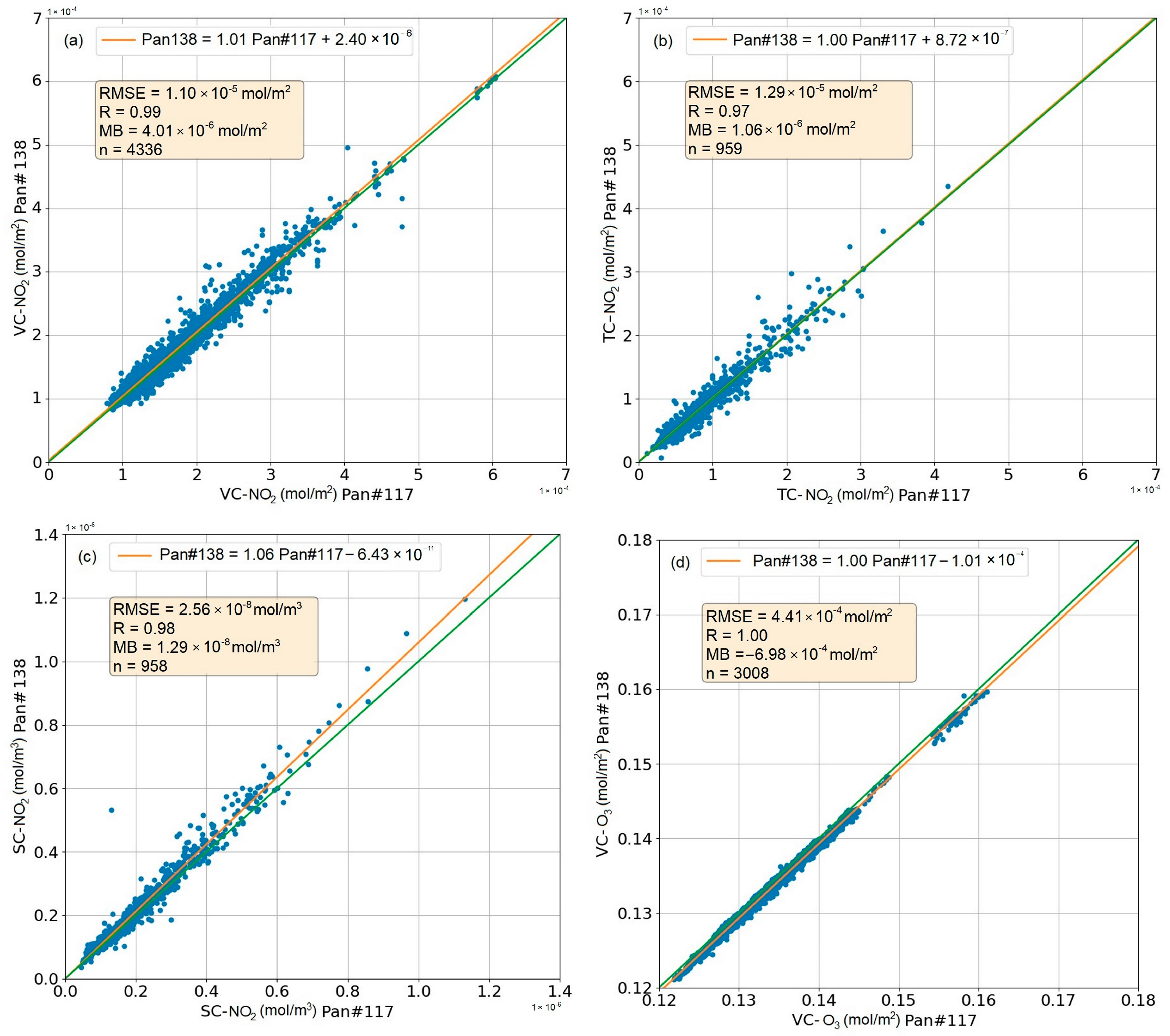
2.3. Data Processing

The screening of PGN NO2 and O3 products is carried out following a three-step procedure: first, data points assigned with data quality levels “high” and “medium” are selected. The segmentation is applied automatically by the data processing software and is based on thresholds of selected retrieval parameters (e.g., the root-mean-square of spectral fitting residuals or wavelength shift). Secondly, the data are screened by requiring a percentage uncertainty smaller than 10% for VC-NO2 and 40% for TC-NO2, SC-NO2, and VC-O3. For direct Sun measurements, the combined, which considers uncertainties with different correlation lengths in time, is used. This includes, amongst others, measurement uncertainty (random uncertainty), cross-section temperature effects, and uncertainties in the estimation of the reference gas content (systematic uncertainty). However, as a rigorous uncertainty budget for MAX-DOAS measurements is very challenging and not provided by PGN, only the measurement uncertainty is considered here. Thirdly, the data retrieved for SZA greater than 80 degrees were discarded.
The VA dataset, being provided as quality-checked by ARPA Lazio, has only been subjected to a visual inspection to exclude any gross errors, such as negative values.
Then, the Pandora and ARPA data were classified as “weekdays”, collected from Monday to Friday, and “weekends”, collected on Saturdays, Sundays, and national holidays. The aim of this division is to take into account the differences in the NO2 and O3 diurnal cycle produced by the traffic reduction during weekends.
Finally, the PGN and ARPA NO2 data are grouped according to their measurement fractional hour in steps of one hour between 00:00 UTC and 23:00 UTC. For each hourly bin, the data average is computed, considering only the time bins in which at least 5 measurements have passed the screening process. This procedure allows for the creation of NO2 VC, TC, and SC plots, as a function of the month of the year and of the hour of the day, using weekdays and weekends data (see Figures S1–S8).

3. Results and Discussion

As discussed in the previous sections, PGN and ARPA Lazio provide columnar and in situ measures, respectively. It is therefore natural to expect differences between the datasets, due to the different working principles of the instruments. Nonetheless, the synergistic use of Pandora and in situ data allows the in-depth investigation of the physical and chemical processes driving the transport and dispersion of pollutants.

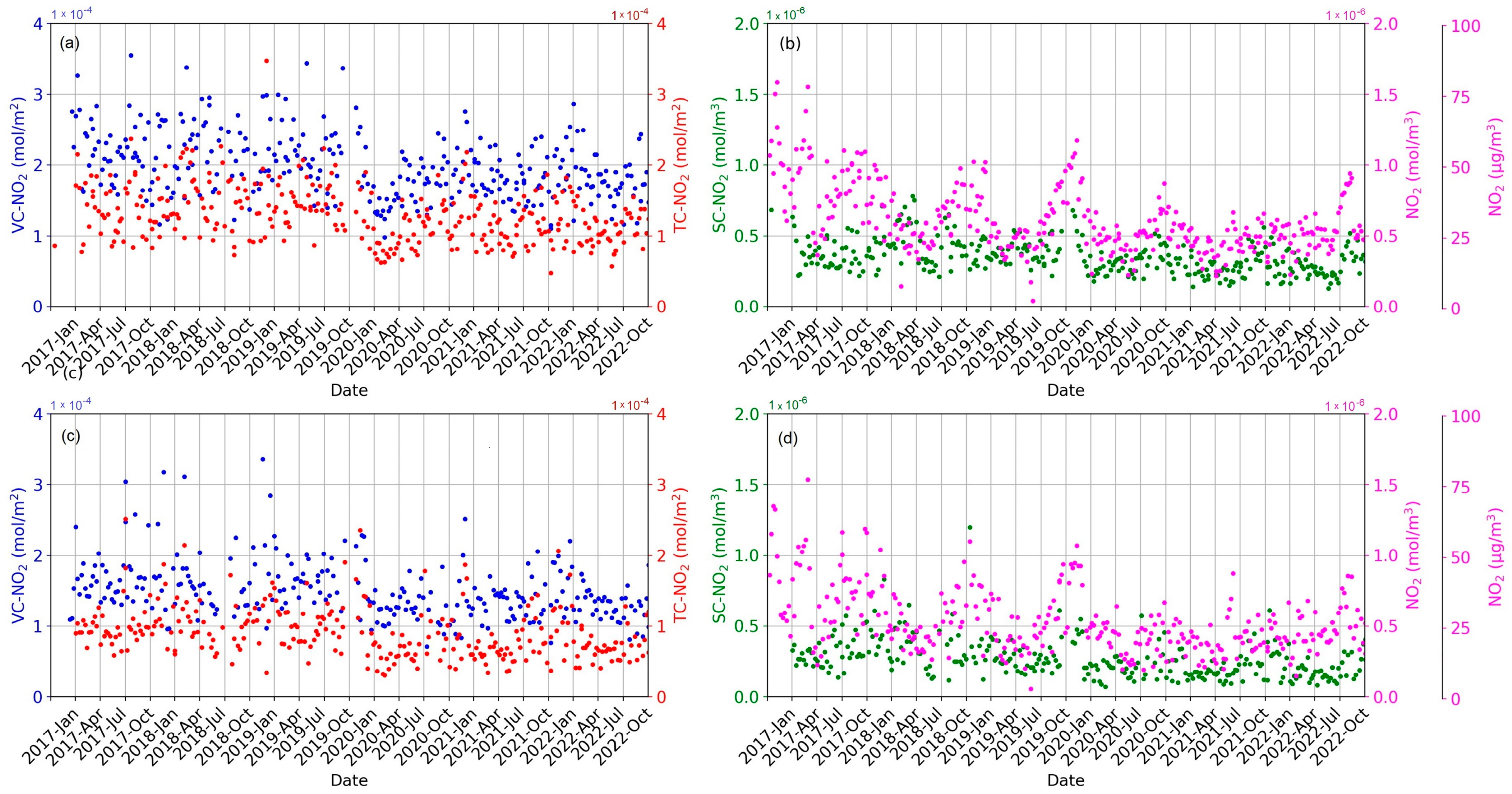
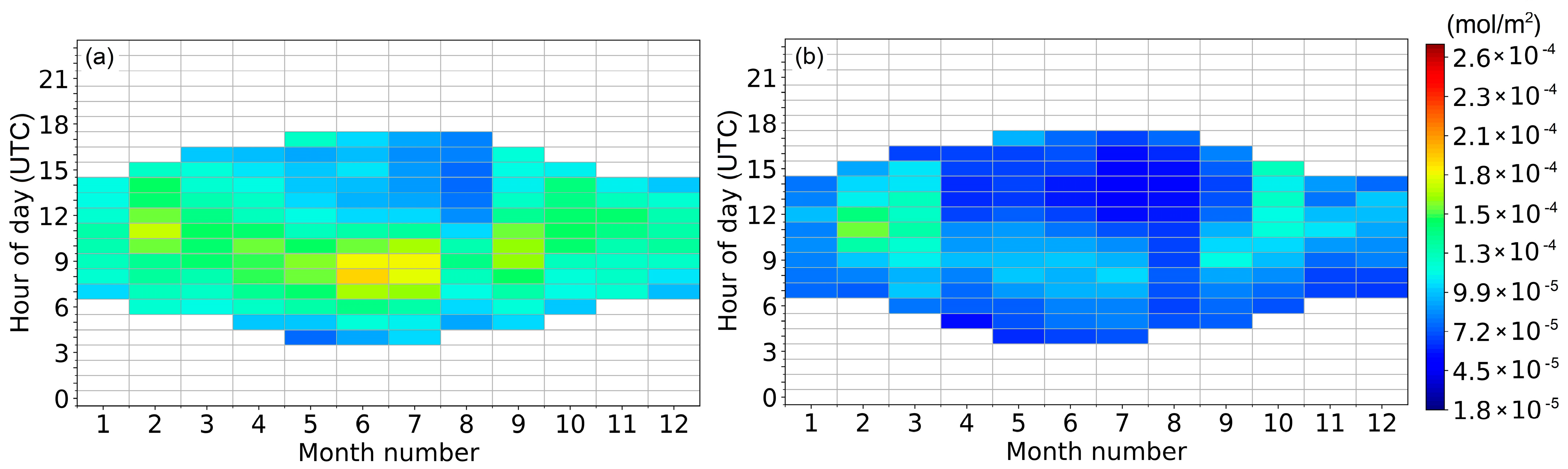
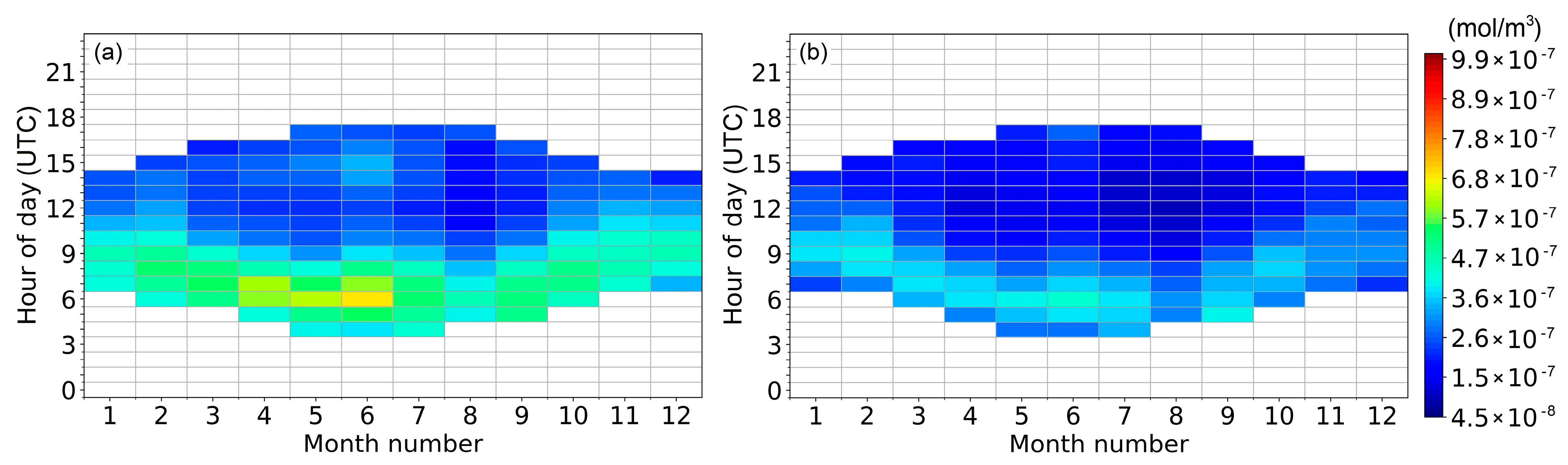
3.1. Nitrogen Dioxide Temporal Variation

Figure 3 depicts the weekly average time series of VC-NO2 and TC-NO2 for weekdays (panel a) and weekends (panel b) and SC-NO2 and in situ NO2 concentrations for weekdays (panel c) and weekends (panel d). It is worth emphasizing that Pandora’s observations are collected only during daylight hours and are screened following the procedure described in Section 2.3, while the VA in situ air quality station operates continuously during the day and night, regardless of weather conditions. Therefore, the weekly averages are computed over a different number of samples and different time ranges.
The plots show some peculiar features, mainly linked to (i) seasonal cyclicality and (ii) inter-annual trends.
For what concerns the seasonal cycle, all the NO2 components assume the highest values during winter, although the seasonal variability is more marked in the in situ and near-surface concentrations rather than in the columnar densities. VC-NO2 and TC-NO2 rarely exceed 3.0 × 10⁻⁴ mol/m2 both on weekdays and weekends although, in the latter case, the values are lower because of the more limited traffic. The trends of VC-NO2 and TC-NO2 agree with [46], who analyzed Pandora data from different locations worldwide, also considering cities at latitudes comparable to Rome. Furthermore, the monthly variation agrees with [29], who studied the NO2 measurements carried out by Pandora and Brewer in Rome, highlighting that the VC-NO2 maxima are recorded in winter due to greater atmospheric stability, reduced tropospheric mixing, oxidation processes, and longer NO2 lifetime as a consequence of the reduced winter irradiance [47].
The seasonal cycle is more evident when observing the in situ and near-surface measurements, as they are more directly affected by the local emissions and photochemical reactions. In Rome, during the cold months, SC-NO2 and in situ NO2 assume quite high values (between 0.2 and 0.8 mol/m3 for SC-NO2 and between 0.4 and 1.6 mol/m3 for in situ NO2). On the contrary, during spring and, above all, summer, the weekly average is lower (about 0.2–0.3 mol/m3 for SC-NO2 and in situ NO2).
The seasonal variations of near-surface and in situ NO2 concentrations are in agreement with [29,48]. Diémoz et al. [29] found a pronounced seasonal variation of SC-NO2 in Rome, with minima in August due to the summer holidays and, therefore, to the closure of industrial and commercial activities, and maxima during winter, attributable to several concomitant factors. First, during winter, the NO2 amount is affected by the increase in anthropogenic emissions because of domestic heating and by slower photochemical reactions [16,49]. Furthermore, the conditions of persistent atmospheric stability and the possible presence of a thermal inversion layer reduce the vertical mixing, inhibiting the dispersion of pollutants [50]. Finally, the atmospheric boundary layer height, which is significantly lower in winter, influences the wind pattern, limiting the dilution of harmful substances in a smaller atmospheric volume and, thus, exacerbating their accumulation close to the ground [38,51]. Voiculescu et al. [48] analyzed the NO2 concentrations measured by traffic stations in the city of Braila (Romania). The seasonal trend is comparable with the one found in Rome, although they highlighted a more marked summer NO2 reduction. This dissimilarity can be attributed to the different extents of the cities analyzed. Braila, in fact, is a small urban center, with a population equal to 8% of that of Rome and an extension of about 2.5%. The anthropogenic sources and the pollutant background of the two cities are therefore not strictly comparable.
Moreover, the time series from 2017 to 2022 show a general decreasing trend of all the columnar and surface components of NO2. This aspect, already discussed by [29,39], can be related to the policies implemented by the Italian and international governance aimed at the progressive tendency towards the replacement of petrol vehicles in favor of hybrid automobiles. Moreover, the access of highly polluting vehicles to the city center has been limited, promoting the use of public transport, as well as cycling and walking. The decreasing trend is more evident in in situ and near-surface data than in columnar values, the latter being more influenced by photochemical reactions and transport.
Finally, Figure 3 highlights the strong effect of the SARS-CoV-2 pandemic on NO2: during the first half of 2020 (i.e., when strict restrictions on private and public travel were implemented in Italy to face the spread of the pandemic), the VC, TC, SC, and in situ amounts of NO2 halved, as also highlighted by [22,52]. Interestingly, the decreasing trend, which began in 2020 because of the pandemic, is still ongoing, although the restrictions on mobility have now been completely lifted. In fact, the NO2 level, after a rapid increase in mid-2020 due to the removal of travel restrictions, has settled at levels lower than that of the pre-pandemic period. This trend has to be further investigated and verified in the next few years, also examining the peculiar conditions affecting Rome in concomitance with the observed maxima and minima. Furthermore, although the NO2 variation is evident both on weekdays and weekends, suggesting independence from meteorological parameters, it would be interesting to analyze the relationship between pollution levels and meteorological variables such as wind intensity, air temperature, and incoming solar radiation. Nonetheless, if confirmed, it would represent an important milestone for the improvement of air quality in Rome, and it would suggest that the pandemic and the related lockdowns might have changed the lifestyle of Roman citizens, improving the quality of urban life. In fact, the introduction of remote working for a non-negligible fraction of citizens could lead to a significant reduction in urban traffic, although a deeper investigation is required to estimate the magnitude of this effect.

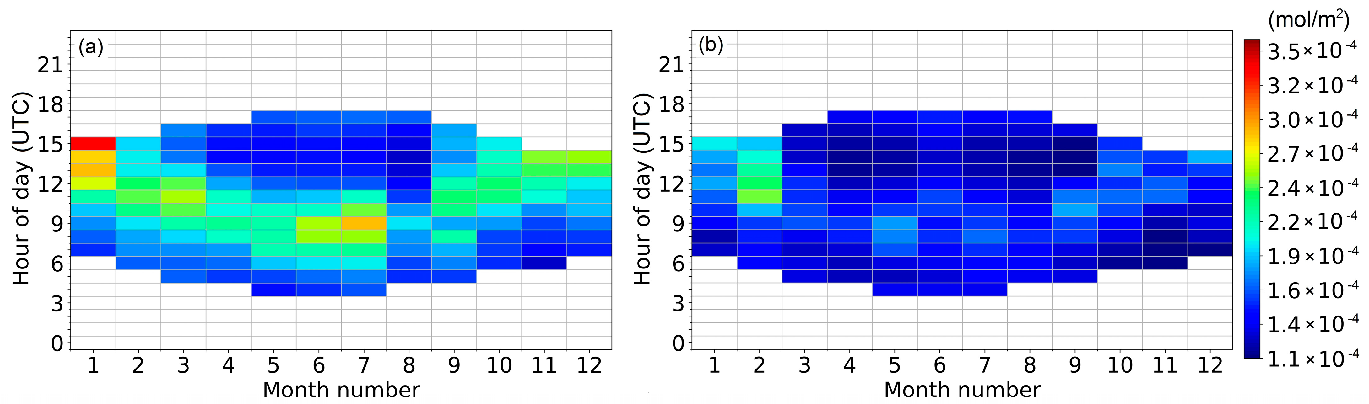
3.2. Analysis of NO2 Daily Peak

Figure 4, Figure 5, Figure 6 and Figure 7 show the VC, TC, SC, and in situ NO2 values as a function of the month of the year and of the hour of the day for workdays and weekends. The results are averaged over the period under investigation, i.e., from 2017 to 2022.
The most relevant feature is the seasonal variation of the NO2 peak value correlated to the Sun illumination over the year. In fact, both during weekdays and weekends, the VC (Figure 4) and TC (Figure 5) peaks are observed at about 13:00 UTC between November and January, and at about 8:00 UTC for June and July. For SC (Figure 6), the peaks follow the same seasonal trend, but the highest values occur approximately three hours before that of columnar contents due to the proximity of the emission sources.
In fact, since the near-surface and the in situ concentration of NO2 are closely linked to local emissions, in the urban area of Rome a morning peak between 07:00 and 09:00 UTC and a second peak between 20:00 and 22:00 UTC, higher than the morning one, are expected [51]. Anyway, Pandora measurements stop just before sunset: during summer, they are limited to about 18:00 UTC while, in the winter months, due to the shorter duration of daytime hours, the measurements typically end at 15:00 UTC, not catching the afternoon peak. Nonetheless, a slight increase in SC-NO2 in the evening hours during the warm months is still noticeable on both weekdays and weekends. The double daily peak is clearly observable from in situ concentrations (Figure 7) provided by the Villa Ada station, which operates routinely, carrying out measurements throughout the day.
The observed diurnal and seasonal variations agree with [48], who observed two diurnal peaks for the NO2 surface concentration at 07:00 UTC and 18:00 UTC, more evident during wintertime, associated with atmospheric dynamics and peaks in vehicular traffic. In fact, as reported by [53], the double peak daily cycle of NO2 is observable in the NO2 concentrations, but not in its vertical fluxes. It suggests that the amount of atmospheric NO2 is mainly driven by the dynamics of the atmospheric boundary layer, and therefore to its development, also in relation to local weather conditions, and only secondarily to the volume of traffic.
Moreover, Figures S1–S8 show NO2 VC, TC, SC, and in situ as a function of time of day and month of the year separately for each year analyzed. The reduction of NO2 over the years, already discussed in Section 3.1, is evident in all the NO2 components, but is more marked in near-surface and in situ NO2, corroborating the idea that the decreasing trend is attributable to the correct implementation of local emission abatement measures.
The described features are visible during both weekdays and weekends, although during weekends the absolute concentrations are lower. The low values recorded during August have no physical–chemical motivation, as they are related to lower vehicular flows due to the summer holidays.

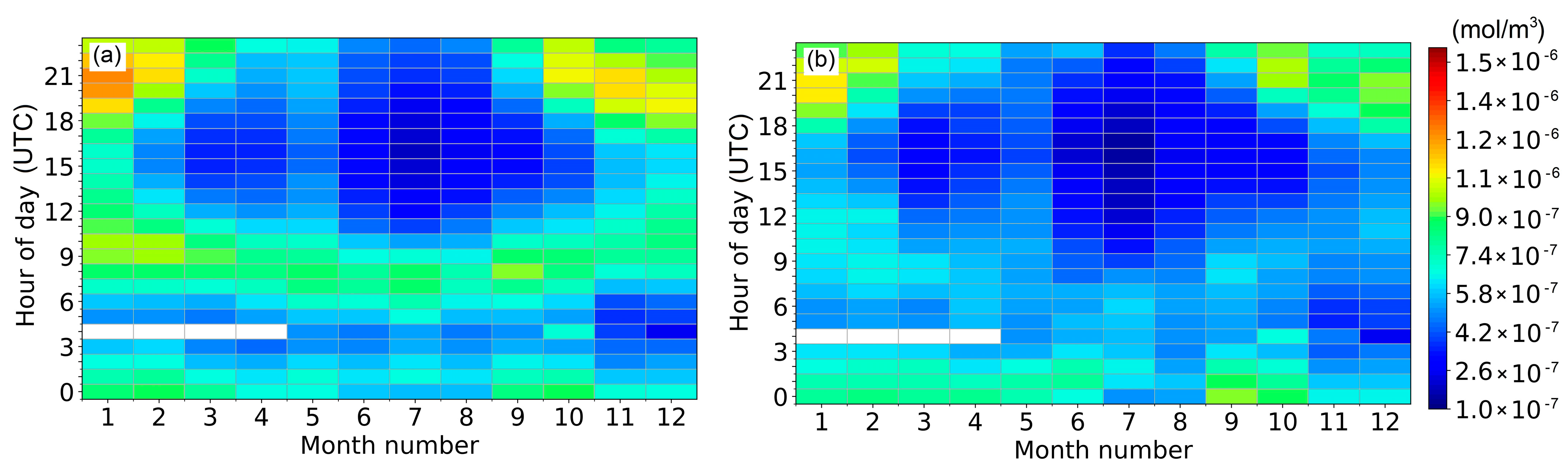
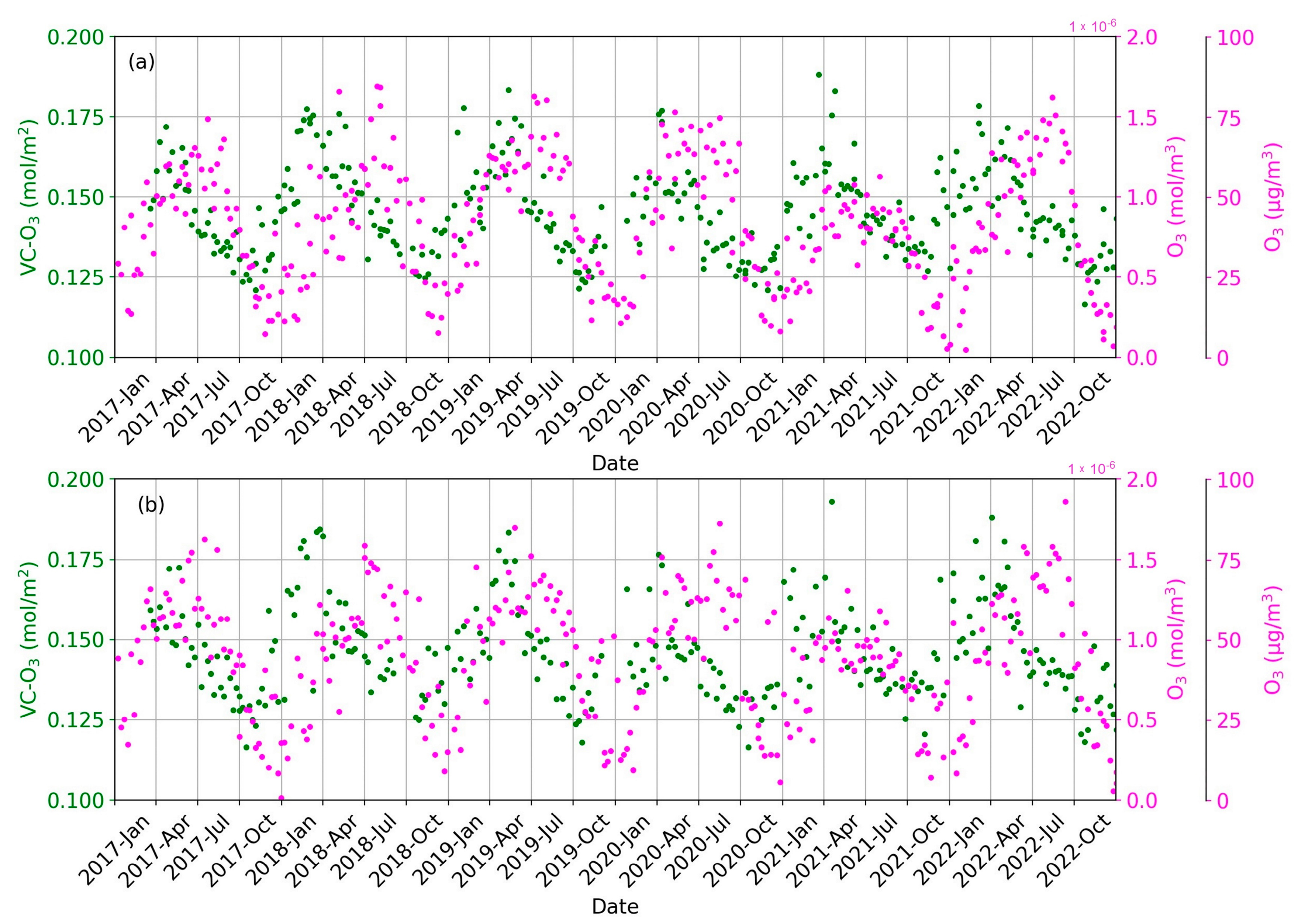
3.3. Ozone Temporal Variation

Figure 8 shows the time series of VC-O3 from Pandora at SAP and the in situ concentration of O3 from the VA station for weekdays (panel a) and weekends (panel b).
Both the vertical density and the in situ concentration of O3 show a clear seasonal cycle, with maxima during summertime and minima during winter. VC-O3 ranges between about 0.12 and 0.19 mol/m2, while the in situ concentration spans between 0.1 × 10⁻⁶ and 1.9 × 10⁻⁶ mol/m3. Although the seasonal variability is clear both from the in situ O3 and VC-O3, a temporal shift of the maxima/minima is noted. This is due to the different processes driving the accumulation and transport of O3 in the atmosphere. In fact, the variability of VC-O3 is mainly associated with the processes occurring in the stratosphere, where most of the O3 is present, and where the VC-O3 is regulated by the balance between the transport associated with the diabatic mean circulation of the stratosphere, or Brewer–Dobson circulation, and photochemical loss [39]. Otherwise, in situ O3, which, unlike stratospheric ozone, is a harmful air pollutant, is essentially linked to the variation of local emissions and photochemical reactions. VC-O3 typically reaches its lowest level during November and December (when transport is dominant), rapidly increasing up to its highest density in spring (when transport decreases and photochemical loss dominates with the increase of solar radiation) and then decreasing during the summer and autumn. Although the spring peak of O3 stratosphere–troposphere exchange has often been observed, recent articles point out that the exchange is not actually limited to just this season [54].
These results agree with [55], who analyzed the diurnal and seasonal cycle of VC-O3 in southern Italy through satellite data and MAX-DOAS ground-based measurements, highlighting the increase of VC-O3 between autumn and spring and the rapid summer decrease. Antòn et al. [56] analyzed the variability of TC-O3 over Portugal, identifying an increase between winter and early spring. In their case, April represents the end of the buildup period, from which the decreasing phase of TC-O3 begins, in agreement with our results and with other studies focused on the northern hemisphere (e.g., [57]). Furthermore, the intense incoming solar radiation during summer favors the titration of O3 by NO and determines the increase of the O3 in situ concentration. On the other hand, in winter, the photochemical reactions are inhibited by the reduced duration of the hours of sunshine and the frequent presence of clouds/rainfalls, resulting in lower levels of O3. Moreover, the processes occurring in the boundary layer and the surface ozone concentrations can be influenced by the vertical transport of stratospheric ozone.
The analysis of long-term time series and the discrimination among weekdays and weekends do not show significant variations in both vertical density and the in situ concentration of O3. The reduction of in situ O3 measured during the summer of 2021 is due to the lower in situ concentrations of NO2, as shown in Figure 3. The absence of the simultaneous reduction in VC-O3 suggests that in situ O3 is mainly determined by local sources and that VC-O3 is driven by transport and stratospheric processes, providing additional and fundamental information for understanding the variations of atmospheric O3 in the framework of climate change [58].

4. Conclusions

In this study, ground-based measurements of NO2 and O3 collected in the center of Rome (Italy) between 2017 and 2022 are analyzed to investigate the inter-annual variability. To study in detail the processes occurring in the atmospheric boundary layer and their relationship with tropospheric and stratospheric pollution levels, both columnar and in situ measurements are considered. Pandora sun-spectrometers provided the time series of VC-NO2, TC-NO2, SC-NO2, and TC-O3, while an urban background air quality station provided the in situ concentrations of NO2 and O3.
The results show that both columnar and in situ amounts of NO2 are decreasing. Possible causes could be the reduction of local emissions thanks to the transition towards electric and hybrid vehicles, as well as the change in the habits of citizens established after the pandemic period.
By observing the hourly and monthly variations of VC-NO2, TC-NO2, SC-NO2 and in situ NO2 for weekdays and workdays for each year of the period under investigation, no inter-annual variations in the time of diurnal NO2 peaks are found, suggesting that the photochemical processes and the NO2 transport mechanisms have remained unchanged over the period analyzed. This corroborates the idea that the decrease of NO2 is attributable to the reduction of local emissions. Furthermore, this suggests that specific traffic calming actions or restricted traffic zones could be implemented during the hours of NO2 peaks.
Otherwise, O3 does not show inter-annual variations, although a marked seasonal cycle is evident. Close to the ground, this variability is attributable to photochemical reactions while, in the columnar density, it might be related to the predominant contribution of stratospheric ozone. The different processes regulating the accumulation and transport of O3 result in a time lag between the peaks of TC-O3 and in situ O3.
Moreover, the evidenced reduction for columnar and in situ NO2 and the constant O3 levels require a more in-depth investigation, also analyzing the absolute concentrations of NOx and VOCs, meteorological parameters, and variations in local emissions, among other factors.
Finally, the analysis of the time series suggests that the policies implemented in recent years and the change in habits caused by the pandemic, such the introduction of remote working, are leading to the reduction of emissions and, therefore, of the NO2 level. With a view to further improve air quality in terms of NO2 and O3, it is crucial to also consider the potential contribution of green infrastructures, such as urban trees [59,60]. Furthermore, the perfect agreement between the data collected by Pandora and the in situ air quality station underlines the importance of the availability of instrumentation in urban environments allowing for the integration of in situ measurements with columnar ones. In fact, the state-of-the-art instrumentation used in this study will soon allow the retrieval of other atmospheric products (such as TC-O3, SC-O3, and formaldehyde), allowing for the study of air pollution in the boundary layer and in the troposphere, investigating the dynamics that govern the transport/accumulation/removal of harmful substances and, therefore, providing useful and cutting-edge tools for assessing the best climate change adaptation measures.

Supplementary Materials

The following supporting information can be downloaded at: https://www.mdpi.com/article/10.3390/atmos14030594/s1, Figure S1: Hourly and monthly variation of VC-NO2 for workdays during 2017 (upper left panel), 2018 (upper right panel), 2019 (central left panel), 2020 (central right panel), 2021 (lower left panel), and 2022 (lower right panel). Figure S2: Hourly and monthly variation of VC-NO2 for weekends during 2017 (upper left panel), 2018 (upper right panel), 2019 (central left panel), 2020 (central right panel), 2021 (lower left panel), and 2022 (lower right panel). Figure S3: Hourly and monthly variation of TC-NO2 for workdays during 2017 (upper left panel), 2018 (upper right panel), 2019 (central left panel), 2020 (central right panel), 2021 (lower left panel), and 2022 (lower right panel). Figure S4: Hourly and monthly variation of TC-NO2 for weekends during 2017 (upper left panel), 2018 (upper right panel), 2019 (central left panel), 2020 (central right panel), 2021 (lower left panel), and 2022 (lower right panel). Figure S5: Hourly and monthly variation of SC-NO2 for workdays during 2017 (upper left panel), 2018 (upper right panel), 2019 (central left panel), 2020 (central right panel), 2021 (lower left panel), and 2022 (lower right panel). Figure S6: Hourly and monthly variation of SC-NO2 for weekends during 2017 (upper left panel), 2018 (upper right panel), 2019 (central left panel), 2020 (central right panel), 2021 (lower left panel), and 2022 (lower right panel). Figure S7: Hourly and monthly variation of in situ NO2 for workdays during 2017 (upper left panel), 2018 (upper right panel), 2019 (central left panel), 2020 (central right panel), 2021 (lower left panel), and 2022 (lower right panel). Figure S8: Hourly and monthly variation of in situ NO2 for weekends during 2017 (upper left panel), 2018 (upper right panel), 2019 (central left panel), 2020 (central right panel), 2021 (lower left panel), and 2022 (lower right panel).

Author Contributions

Conceptualization, A.D.B., S.C. and A.M.I.; methodology, A.D.B., S.C. and A.M.I.; software, G.M. and A.D.B.; validation, G.M., A.C. and M.T.; formal analysis, A.D.B., G.M., S.C. and A.M.I.; investigation, A.D.B. and G.M.; resources, G.M. and S.C.; data curation, A.C., M.T., G.M., A.M.I., S.C. and A.D.B.; writing—original draft preparation, A.D.B.; writing—review and editing, A.D.B., A.M.I., G.M., S.F., A.C., M.T. and S.C.; visualization, G.M. and A.D.B.; supervision, S.C.; project administration, S.C.; funding acquisition, S.C. All authors have read and agreed to the published version of the manuscript.

Funding

This research was supported by BAQUNIN Project team, funded by ESA through the contract ID 4000126749/19/I-NS. Serena Falasca was funded by MUR (Ministero dell’Università e della Ricerca of Italy) under PON “Ricerca e Innovazione” 2014–2020 (D.M. 1062/2021).

Institutional Review Board Statement

Not applicable.

Informed Consent Statement

Not applicable.

Data Availability Statement

The Pandora PGN datasets analyzed during the current study are available at https://www.pandonia-global-network.org/ (accessed on 20 March 2023). In situ air quality datasets are available at http://www.arpalazio.net/main/aria/sci/basedati/chimici/chimici.php (accessed on 20 March 2023).

Acknowledgments

The authors gratefully acknowledge Angelika Dehn and Philippe Goryl from ESA EOP-GMQ SPPA for their scientific and financial support. The authors thank PGN, a bilateral project supported with funding from the National Aeronautics and Space Administration (NASA) and ESA, for providing columnar densities and near-surface concentrations of NO2 and O3 and ARPA Lazio for providing in situ concentrations of NO2 and O3.

Conflicts of Interest

The authors declare no conflict of interest.

References

  1. WHO Regional Office for Europe. WHO Global Air Quality Guidelines: Particulate Matter (PM2.5 and PM10), ozone, Nitrogen Dioxide, Sulfur Dioxide and Carbon Monoxide. World Health Organization. Regional Office for Europe. 2021. Available online: https://apps.who.int/iris/handle/10665/345329 (accessed on 30 January 2023).
  2. Kuehn, B.M. WHO: More than 7 million air pollution deaths each year. JAMA 2014, 311, 1486. [Google Scholar] [CrossRef]
  3. Ancelet, T.; Davy, P.K.; Trompetter, W.J.; Markwitz, A. Sources of particulate matter pollution in a small New Zealand city. Atmos. Pollut. Res. 2014, 5, 572–580. [Google Scholar] [CrossRef] [Green Version]
  4. Williams, A.G.; Chambers, S.D.; Conen, F.; Reimann, S.; Hill, M.; Griffiths, A.D.; Crawford, J. Radon as a tracer of atmospheric influences on traffic-related air pollution in a small inland city. Tellus B 2016, 68, 30967. [Google Scholar] [CrossRef] [Green Version]
  5. Ponomarev, N.; Yushkov, V.; Elansky, N. Air Pollution in Moscow Megacity: Data Fusion of the Chemical Transport Model and Observational Network. Atmosphere 2021, 12, 374. [Google Scholar] [CrossRef]
  6. Karuppasamy, M.B.; Natesan, U.; Karuppannan, S.; Chandrasekaran, L.N.; Hussain, S.; Almohamad, H.; Al Dughairi, A.A.; Al-Mutiry, M.; Alkayyadi, I.; Abdo, H.G. Multivariate Urban Air Quality Assessment of Indoor and Outdoor Environments at Chennai Metropolis in South India. Atmosphere 2022, 13, 1627. [Google Scholar] [CrossRef]
  7. Yang, J.; Shi, B.; Shi, Y.; Marvin, S.; Zheng, Y.; Xia, G. Air pollution dispersal in high density urban areas: Research on the triadic relation of wind, air pollution, and urban form. Sustain. Cities Soc. 2020, 54, 101941. [Google Scholar] [CrossRef]
  8. Nardecchia, F.; Di Bernardino, A.; Pagliaro, F.; Monti, P.; Leuzzi, G.; Gugliermetti, L. CFD analysis of urban canopy flows employing the V2F model: Impact of different aspect ratios and relative heights. Adv. Meteorol. 2018, 2018, 2189234. [Google Scholar] [CrossRef]
  9. Miao, C.; Yu, S.; Zhang, Y.; Hu, Y.; He, X.; Chen, W. Assessing outdoor air quality vertically in an urban street canyon and its response to microclimatic factors. J. Environ. Sci. 2023, 124, 923–932. [Google Scholar] [CrossRef]
  10. European Union. Council Directive 1999/30/EC of 22 April 1999 Relating to Limit Values for Sulphur Dioxide, Nitrogen Dioxide and Oxides of Nitrogen, Particulate Matter and Lead in Ambient Air; Official Journal of the European Communities, En Series. 1999. Available online: http://data.europa.eu/eli/dir/1999/30/oj (accessed on 15 March 2023).
  11. European Union. Directive 2008/50/EC of the European Parliament and of the Council of 21 May 2008 on Ambient Air Quality and Cleaner Air for Europe; Official Journal of the European Communities, En Series. 2008. Available online: http://data.europa.eu/eli/dir/2008/50/oj (accessed on 15 March 2023).
  12. Karlsson, P.E.; Klingberg, J.; Engardt, M.; Andersson, C.; Langner, J.; Karlsson, G.P.; Pleijel, H. Past, present and future concentrations of ground-level ozone and potential impacts on ecosystems and human health in northern Europe. Sci. Total Environ. 2017, 576, 22–35. [Google Scholar] [CrossRef]
  13. Huo, M.; Yamashita, K.; Chen, F.; Sato, K. Spatial-Temporal Variation in Health Impact Attributable to PM2. 5 and Ozone Pollution in the Beijing Metropolitan Region of China. Atmosphere 2022, 13, 1813. [Google Scholar] [CrossRef]
  14. Kumari, S.; Lakhani, A.; Kumari, K.M. First observation-based study on surface O3 trend in Indo-Gangetic Plain: Assessment of its impact on crop yield. Chemosphere 2020, 255, 126972. [Google Scholar] [CrossRef] [PubMed]
  15. Beirle, S.; Boersma, K.F.; Platt, U.; Lawrence, M.G.; Wagner, T. Megacity emissions and lifetimes of nitrogen oxides probed from space. Science 2011, 333, 1737–1739. [Google Scholar] [CrossRef] [PubMed]
  16. Beirle, S.; Platt, U.; Wenig, M.; Wagner, T. Weekly cycle of NO2 by GOME measurements: A signature of anthropogenic sources. Atmos. Chem. Phys. 2003, 3, 2225–2232. [Google Scholar] [CrossRef] [Green Version]
  17. Air Quality Europe 2022 Report. Available online: https://www.eea.europa.eu/publications/air-quality-in-europe-2022/sources-and-emissions-of-air (accessed on 31 January 2023).
  18. Sharma, S.; Sharma, P.; Khare, M. Photo-chemical transport modelling of tropospheric ozone: A review. Atmos. Environ. 2017, 159, 34–54. [Google Scholar] [CrossRef]
  19. Karl, T.; Lamprecht, C.; Graus, M.; Cede, A.; Tiefengraber, M.; Vila-Guerau de Arellano, J.; Gurarie, D.; Lenschow, D. High urban NOx triggers a substantial chemical downward flux of ozone. Sci. Adv. 2023, 9, eadd2365. [Google Scholar] [CrossRef] [PubMed]
  20. Lal, S.; Naja, M.; Subbaraya, B.H. Seasonal variations in surface ozone and its precursors over an urban site in India. Atmos. Environ. 2000, 34, 2713–2724. [Google Scholar] [CrossRef]
  21. Han, S.; Bian, H.; Feng, Y.; Liu, A.; Li, X.; Zeng, F.; Zhang, X. Analysis of the relationship between O3, NO and NO2 in Tianjin, China. Aerosol Air Qual. Res. 2011, 11, 128–139. [Google Scholar] [CrossRef] [Green Version]
  22. Campanelli, M.; Iannarelli, A.M.; Mevi, G.; Casadio, S.; Diémoz, H.; Finardi, S.; Dinoi, A.; Castelli, E.; di Sarra, A.; Di Bernardino, A.; et al. A wide-ranging investigation of the COVID-19 lockdown effects on the atmospheric composition in various Italian urban sites (AER–LOCUS). Urban Clim. 2021, 39, 100954. [Google Scholar] [CrossRef]
  23. SciGlob Instruments and Services LLC. Available online: https://sciglob.com/ (accessed on 7 February 2023).
  24. Herman, J.; Cede, A.; Spinei, E.; Mount, G.; Tzortziou, M.; Abuhassan, N. NO2 column amounts from ground-based Pandora and MFDOAS spectrometers using the direct-sun DOAS technique: Intercomparisons and application to OMI validation. J. Geophys. Res. 2009, 114, D13307. [Google Scholar] [CrossRef] [Green Version]
  25. Pandonia Global Network. Available online: https://www.pandonia-global-network.org/ (accessed on 31 January 2023).
  26. Thompson, A.M.; Stauffer, R.M.; Boyle, T.P.; Kollonige, D.E.; Miyazaki, K.; Tzortziou, M.; Herman, J.R.; Abuhassan, N.; Jordan, C.E.; Lamb, B.T. Comparison of near-surface NO2 pollution with pandora total column NO2 during the Korea-United States ocean color (KORUS OC) campaign. J. Geophys. Res. Atmos. 2019, 124, 13560–13575. [Google Scholar] [CrossRef]
  27. Judd, L.M.; Al-Saadi, J.A.; Szykman, J.J.; Valin, L.C.; Janz, S.J.; Kowalewski, M.G.; Esker, H.J.; Veefkind, J.P.; Cede, A.; Mueller, M.; et al. Evaluating Sentinel-5P TROPOMI tropospheric NO2 column densities with airborne and Pandora spectrometers near New York City and Long Island Sound. Atmos. Meas. Tech. 2020, 13, 6113–6140. [Google Scholar] [CrossRef]
  28. Wang, S.; Pongetti, T.J.; Sander, S.P.; Spinei, E.; Mount, G.H.; Cede, A.; Herman, J. Direct Sun measurements of NO2 column abundances from Table Mountain, California: Intercomparison of low-and high-resolution spectrometers. J. Geophys. Res. Atmos. 2010, 115, D13305. [Google Scholar] [CrossRef] [Green Version]
  29. Diémoz, H.; Siani, A.M.; Casadio, S.; Iannarelli, A.M.; Casale, G.R.; Savastiouk, V.; Cede, A.; Tiefengraber, M.; Müller, M. Advanced NO2 retrieval technique for the Brewer spectrophotometer applied to the 20-year record in Rome, Italy. Earth Syst. Sci. Data 2021, 13, 4929–4950. [Google Scholar] [CrossRef]
  30. Tzortziou, M.; Herman, J.R.; Cede, A.; Loughner, C.P.; Abuhassan, N.; Naik, S. Spatial and temporal variability of ozone and nitrogen dioxide over a major urban estuarine ecosystem. J. Atmos. Chem. 2015, 72, 287–309. [Google Scholar] [CrossRef]
  31. Di Bernardino, A.; Iannarelli, A.M.; Casadio, S.; Mevi, G.; Campanelli, M.; Casasanta, G.; Cede, A.; Tiefengraber, M.; Siani, A.M.; Spinei, E.; et al. On the effect of sea breeze regime on aerosols and gases properties in the urban area of Rome, Italy. Urban Clim. 2021, 37, 100842. [Google Scholar] [CrossRef]
  32. Beck, H.E.; Zimmermann, N.E.; McVicar, T.R.; Vergopolan, N.; Berg, A.; Wood, E.F. Present and future Köppen-Geiger climate classification maps at 1-km resolution. Sci. Data 2018, 5, 180214. [Google Scholar] [CrossRef] [Green Version]
  33. Petenko, I.; Mastrantonio, G.; Viola, A.; Argentini, S.; Coniglio, L.; Monti, P.; Leuzzi, G. Local circulation diurnal patterns and their relationship with large-scale flows in a coastal area of the Tyrrhenian Sea. Bound.-Layer Meteorol. 2011, 139, 353–366. [Google Scholar] [CrossRef]
  34. Ciardini, V.; Di Iorio, T.; Di Liberto, L.; Tirelli, C.; Casasanta, G.; di Sarra, A.; Fiocco, G.; Fuà, D.; Cacciani, M. Seasonal variability of tropospheric aerosols in Rome. Atmos. Res. 2012, 118, 205–214. [Google Scholar] [CrossRef]
  35. Iannarelli, A.M.; Di Bernardino, A.; Casadio, S.; Bassani, C.; Cacciani, M.; Campanelli, M.; Casasanta, G.; Cadau, E.; Diémoz, H.; Mevi, G.; et al. The Boundary Layer Air Quality-Analysis Using Network of Instruments (BAQUNIN) Supersite for Atmospheric Research and Satellite Validation over Rome Area. Bull. Am. Meteorol. Soc. 2022, 103, E599–E618. [Google Scholar] [CrossRef]
  36. Boundary-Layer Air Quality-Analysis Using Network of Instruments Atmospheric Observatory. Available online: https://www.baqunin.eu/ (accessed on 30 January 2023).
  37. Fabrizi, R.; Bonafoni, S.; Biondi, R. Satellite and ground-based sensors for the urban heat island analysis in the city of Rome. Remote Sens. 2010, 2, 1400–1415. [Google Scholar] [CrossRef] [Green Version]
  38. Gariazzo, C.; Silibello, C.; Finardi, S.; Radice, P.; Piersanti, A.; Calori, G.; Cecinato, A.; Perrino, C.; Nussio, F.; Cagnoli, M.; et al. A gas/aerosol air pollutants study over the urban area of Rome using a comprehensive chemical transport model. Atmos. Environ. 2007, 41, 7286–7303. [Google Scholar] [CrossRef]
  39. Di Bernardino, A.; Iannarelli, A.M.; Diémoz, H.; Casadio, S.; Cacciani, M.; Siani, A.M. Analysis of two-decade meteorological and air quality trends in Rome (Italy). Theor. Appl. Climatol. 2022, 149, 291–307. [Google Scholar] [CrossRef] [PubMed]
  40. Italian Legislative Decree 30 March 2017 GU n. 96. Available online: https://www.gazzettaufficiale.it/eli/id/2017/04/26/17A02825/sg (accessed on 30 January 2023).
  41. Cede, A. Manual for Blick Software Suite Version 12. 2019. Available online: https://www.pandonia-global-network.org/wp-content/uploads/2019/11/BlickSoftwareSuite_Manual_v1-7.pdf (accessed on 30 January 2023).
  42. Cede, A.; Tiefengraber, M.; Gebetsberger, M.; Kreuter, A. LuftBlick_FRM4AQ_PGNUserGuidelines_RP_2019009_v1. Available online: https://www.pandonia-global-network.org/wp-content/uploads/2020/01/LuftBlick_FRM4AQ_PGNUserGuidelines_RP_2019009_v1.pdf (accessed on 30 January 2023).
  43. Cede, A.; Tiefengraber, M.; Gebetsberger, M.; Spinei Lind, E. Pandonia Global Network Data Products Readme Document. Available online: https://www.pandonia-global-network.org/wp-content/uploads/2022/12/PGN_DataProducts_Readme_v1-8-6.pdf (accessed on 20 February 2023).
  44. Hönninger, G.; von Friedeburg, C.; Platt, U. Multi axis differential optical absorption spectroscopy (MAX-DOAS). Atmos. Chem. Phys. 2004, 4, 231–254. [Google Scholar] [CrossRef] [Green Version]
  45. Spinei, E.; Tiefengraber, M.; Müller, M.; Cede, A.; Berkhout, S.; Dong, Y.; Nowak, N. Simple retrieval of atmospheric trace gas vertical concentration profiles from multi-axis DOAS observations. 2020; in preparation. [Google Scholar]
  46. Herman, J.; Abuhassan, N.; Kim, J.; Kim, J.; Dubey, M.; Raponi, M.; Tzortziou, M. Underestimation of column NO2 amounts from the OMI satellite compared to diurnally varying ground-based retrievals from multiple PANDORA spectrometer instruments. Atmos. Meas. Tech. 2019, 12, 5593–5612. [Google Scholar] [CrossRef] [Green Version]
  47. Shah, V.; Jacob, D.J.; Li, K.; Silvern, R.F.; Zhai, S.; Liu, M.; Lin, J.; Zhang, Q. Effect of changing NOx lifetime on the seasonality and long-term trends of satellite-observed tropospheric NO2 columns over China. Atmos. Chem. Phys. 2020, 20, 1483–1495. [Google Scholar] [CrossRef] [Green Version]
  48. Voiculescu, M.; Constantin, D.E.; Condurache-Bota, S.; Călmuc, V.; Roșu, A.; Dragomir Bălănică, C.M. Role of meteorological parameters in the diurnal and seasonal variation of NO2 in a Romanian urban environment. Int. J. Environ. Res. Public Health 2020, 17, 6228. [Google Scholar] [CrossRef]
  49. Anand, J.S.; Monks, P.S. Estimating daily surface NO2 concentrations from satellite data—A case study over Hong Kong using land use regression models. Atmos. Chem. Phys. 2017, 17, 8211–8230. [Google Scholar] [CrossRef] [Green Version]
  50. Cattani, G.; di Bucchianico, A.D.M.; Dina, D.; Inglessis, M.; Notaro, C.; Settimo, G.; Viviano, G.; Marconi, A. Evaluation of the temporal variation of air quality in Rome, Italy from 1999 to 2008. Ann. Ist. Super. Sanità 2010, 46, 242–253. [Google Scholar]
  51. Pichelli, E.; Ferretti, R.; Cacciani, M.; Siani, A.M.; Ciardini, V.; Di Iorio, T. The role of urban boundary layer investigated with high-resolution models and ground-based observations in Rome area: A step towards understanding parameterization potentialities. Atmos. Meas. Tech. 2014, 7, 315–332. [Google Scholar] [CrossRef] [Green Version]
  52. Bassani, C.; Vichi, F.; Esposito, G.; Montagnoli, M.; Giusto, M.; Ianniello, A. Nitrogen dioxide reductions from satellite and surface observations during COVID-19 mitigation in Rome (Italy). Environ. Sci. Pollut. Res. 2021, 28, 22981–23004. [Google Scholar] [CrossRef] [PubMed]
  53. Karl, T.; Graus, M.; Striednig, M.; Lamprecht, C.; Hammerle, A.; Wohlfahrt, G.; Held, A.; von der Heyden, L.; Deventer, M.J.; Krismer, A.; et al. Urban eddy covariance measurements reveal significant missing NOx emissions in Central Europe. Sci. Rep. 2017, 7, 2536. [Google Scholar] [CrossRef] [PubMed] [Green Version]
  54. Cristofanelli, P.; Bonasoni, P.; Tositti, L.; Bonafe, U.; Calzolari, F.; Evangelisti, F.; Sandrini, S.; Stohl, A. A 6-year analysis of stratospheric intrusions and their influence on ozone at Mt. Cimone (2165 m above sea level). J. Geophys. Res. Atmos. 2006, 111, D03306. [Google Scholar] [CrossRef] [Green Version]
  55. Pettinari, P.; Donateo, A.; Papandrea, E.; Bortoli, D.; Pappaccogli, G.; Castelli, E. Analysis of NO2 and O3 Total Columns from DOAS Zenith-Sky Measurements in South Italy. Remote Sens. 2022, 14, 5541. [Google Scholar] [CrossRef]
  56. Antón, M.; Bortoli, D.; Costa, M.J.; Kulkarni, P.S.; Domingues, A.F.; Barriopedro, D.; Serrano, A.; Silva, A.M. Temporal and spatial variabilities of total ozone column over Portugal. Remote Sens. Environ. 2011, 115, 855–863. [Google Scholar] [CrossRef]
  57. Schmalwieser, A.W.; Schauberger, G.; Janouch, M. Temporal and spatial variability of total ozone content over Central Europe: Analysis in respect to the biological effect on plants. Agric. For. Meteorol. 2003, 120, 9–26. [Google Scholar] [CrossRef]
  58. Barnes, P.W.; Williamson, C.E.; Lucas, R.M.; Robinson, S.A.; Madronich, S.; Paul, N.D.; Borman, J.F.; Bais, A.F.; Sulzberger, B.; Wilson, S.R.; et al. Ozone depletion, ultraviolet radiation, climate change and prospects for a sustainable future. Nat. Sustain. 2019, 2, 569–579. [Google Scholar] [CrossRef] [Green Version]
  59. Fusaro, L.; Mereu, S.; Salvatori, E.; Agliari, E.; Fares, S.; Manes, F. Modeling ozone uptake by urban and peri-urban forest: A case study in the Metropolitan City of Rome. Environ. Sci. Pollut. Res. 2018, 25, 8190–8205. [Google Scholar] [CrossRef]
  60. Kašpar, V.; Zapletal, M.; Samec, P.; Komárek, J.; Bílek, J.; Juráň, S. Unmanned aerial systems for modelling air pollution removal by urban greenery. Urban For. Urban Green. 2022, 78, 127757. [Google Scholar] [CrossRef]
Figure 1. (a) Geographical map of the area under investigation. The black dashed line depicts the urban center of Rome, and cyan and magenta markers show the positions of the Sapienza (SAP) and Villa Ada (VA) stations. (b) Aerial photograph of the area surrounding Sapienza (SAP). (c) Aerial photograph of the area surrounding Villa Ada (VA).
Atmosphere 14 00594 g001
Figure 2. Pan#138 vs. Pan#117 scatter plots for the period 24 July—11 September 2020 (a) VC-NO2, (b) TC-NO2, (c) SC-NO2, and (d) VC-O3. The reported statistical parameters are root-mean-square of differences (RMSE), linear Pearson correlation coefficient (R), mean bias (MB), and number of valid retrievals (n). Orange lines indicate the linear fit between the two instruments, while green lines indicate the ideal fit y = x .
Atmosphere 14 00594 g002
Figure 3. Weekly average time series of VC-NO2 and TC-NO2 for (a) weekdays and (b) weekends and SC-NO2 and in situ NO2 concentration for (c) weekdays and (d) weekends. VC-NO2, TC-NO2, and SC-NO2 are measured at Sapienza (SAP) from Pandora. In situ NO2 concentrations are measured at the Villa Ada (VA) station.
Atmosphere 14 00594 g003
Figure 4. Hourly and monthly variation of VC-NO2 for (a) weekdays and (b) weekends over the period 2017–2022.
Atmosphere 14 00594 g004
Figure 5. Hourly and monthly variation of TC-NO2 for (a) weekdays and (b) weekends over the period 2017–2022.
Atmosphere 14 00594 g005
Figure 6. Hourly and monthly variation of SC-NO2 for (a) weekdays and (b) weekends over the period 2017–2022.
Atmosphere 14 00594 g006
Figure 7. Hourly and monthly variation of in situ NO2 for (a) weekdays and (b) weekends over the period 2017–2022.
Atmosphere 14 00594 g007
Figure 8. Weekly average time series of VC-O3 and in situ O3 concentration for (a) weekdays and (b) weekends. VC-O3 is measured at Sapienza (SAP) from Pandora. In situ O3 concentration is measured at the Villa Ada (VA) station.
Atmosphere 14 00594 g008
Disclaimer/Publisher’s Note: The statements, opinions and data contained in all publications are solely those of the individual author(s) and contributor(s) and not of MDPI and/or the editor(s). MDPI and/or the editor(s) disclaim responsibility for any injury to people or property resulting from any ideas, methods, instructions or products referred to in the content.

