Article

Apportionment of PM2.5 Sources across Sites and Time Periods: An Application and Update for Detroit, Michigan

1
Department of Biostatistics, University of Michigan, Ann Arbor, MI 48109, USA
2
Department of Environmental Health Sciences, University of Michigan, Ann Arbor, MI 48109, USA
*
Author to whom correspondence should be addressed.
Atmosphere 2023, 14(3), 592; https://doi.org/10.3390/atmos14030592
Submission received: 14 February 2023 / Revised: 9 March 2023 / Accepted: 15 March 2023 / Published: 20 March 2023
(This article belongs to the Special Issue The Michigan-Ontario Ozone Source Experiment (MOOSE))

Abstract

:
Identifying sources of air pollutants is essential for informing actions to reduce emissions, exposures, and adverse health impacts. This study updates and extends apportionments of particulate matter (PM2.5) in Detroit, MI, USA, an area with extensive industrial, vehicular, and construction activity interspersed among vulnerable communities. We demonstrate an approach that uses positive matrix factorization models with combined spatially and temporally diverse datasets to assess source contributions, trend seasonal levels, and examine pandemic-related effects. The approach consolidates measurements from 2016 to 2021 collected at three sites. Most PM2.5 was due to mobile sources, secondary sulfate, and secondary nitrate; smaller contributions arose from soil/dust, ferrous and non-ferrous metals, and road salt sources. Several sources varied significantly by season and site. Pandemic-related changes were generally modest. Results of the consolidated models were more consistent with respect to trends and known sources, and the larger sample size should improve representativeness and stability. Compared to earlier apportionments, contributions of secondary sulfate and nitrate were lower, and mobile sources now represent the dominant PM2.5 contributor. We show the growing contribution of mobile sources, the need to update apportionments performed just 5–10 years ago, and that apportionments at a single site may not apply elsewhere in the same urban area, especially for local sources.

1. Introduction

Identifying the sources of ambient air pollutants is essential for undertaking actions to reduce the emissions, exposures, and health effects associated with pollutant exposure [1,2,3,4]. Approaches used to derive the source apportionments that provide this understanding include the use of receptor models [5,6,7,8] that apportion particulate matter (PM2.5) to source categories that include, as examples: soil/dust and other geological/crustal materials [9,10]; secondary pollutants containing sulfate and nitrate; road wear [11]; traffic and woodsmoke associated with organic and elemental carbon (OC, EC) [12]; ocean-derived aerosols associated with sodium chloride [13]; and incinerator and other industrial emissions associated with refractory and heavy metals [14,15,16,17,18]. Contributions from such sources can vary over both time and space, reflecting the locations, emission rates, and compositions of both local and distant sources, as well as meteorological factors that affect transport, formation, and fate of pollutants. Examples of notable changes that have reduced emissions include use of low- and ultra-low-sulfur fuels (phased in from about 2006–2014), adoption of diesel particulate filters (after 2017), retirement of aging coal and oil boilers (2000 to present, often replaced by gas turbines after 2015), and gradual electrification of the vehicle fleet (ongoing). These long-term trends are modified by economic and construction cycles (e.g., increased activity and emissions during warmer seasons and economic upturns) and seasonal patterns that govern agricultural and biogenic emissions as well as wildland fires. Both long-term and seasonal changes may limit the relevance of apportionments performed just a decade ago. Further, due to spatial variability, appointments obtained using receptor modeling and chemical speciation data collected at a single location may not apply at other locations, even in the same urban area, unless the data are broadly representative of the distribution and impact of emission sources. Unfortunately, sites that measure and speciate PM are sparsely situated, and, often, only a single location in an urban area is available. In consequence, most apportionments using receptor modeling have been based on monitoring data collected at a single site, even in large urban areas, and the understanding of intraurban spatial differences is limited.
This study’s goals are to assess and contrast annual and seasonal apportionments of PM2.5 at multiple sites in an urban area, to examine recent trends, including those related to the pandemic that affected both traffic and industry, and to contrast apportionments obtained using several modeling approaches. The study area focuses on Detroit, MI, USA, an area with long-standing environmental justice issues due to the density of industry, the high fraction of African-American, Hispanic, and Arab-American populations, and the generally poorer health of these communities, including elevated rates of asthma and other pollutant-related diseases, relative to rates in nearby areas. The area has been in nonattainment for the SO2 (since 2013) and the ozone (since 2018) National Ambient Air Quality Standards. Local epidemiological studies have linked air pollution to allergic airway disease [19], cardiovascular and respiratory mortality [20], adverse birth outcomes [21], asthma and lung function [22,23]. Health surveillance data show considerably elevated rates of asthma and asthma-related deaths [24].
Prior studies in Detroit have identified traffic-related emissions, secondary sulfate, and secondary nitrate as the top PM2.5 sources, but the estimated contributions have varied greatly. For example, an analysis of 1999–2002 data collected at two schools (Mayberry in Southwest Detroit and Keith in Eastside Detroit) showed that secondary sulfate comprised 66.3 and 60.1% of PM2.5 at the two sites, respectively, and that motor vehicles contributed 30.9 and 23.4% [25]. Secondary nitrate was not identified as a contributor. Four more recent studies have reported fairly consistent results at Allen Park, a site ~7 km southwest of Detroit: 27–33% of PM2.5 was secondary sulfate; 21–28% was secondary nitrate; and 19–38% was vehicle-related [16,26,27,28]. At Dearborn, a heavily industrialized area adjacent to Detroit, 2002–2005 data were used to estimate secondary sulfate, secondary nitrate, and mobile contributions of 23, 20, and 22%, respectively [27]; a subsequent short-term (29 days) study in 2007 shifted these contributions to 34, 7, and 5%, respectively [17]. Notably, none of these studies used recent data, and none addressed spatial differences within the airshed.

2. Materials and Methods

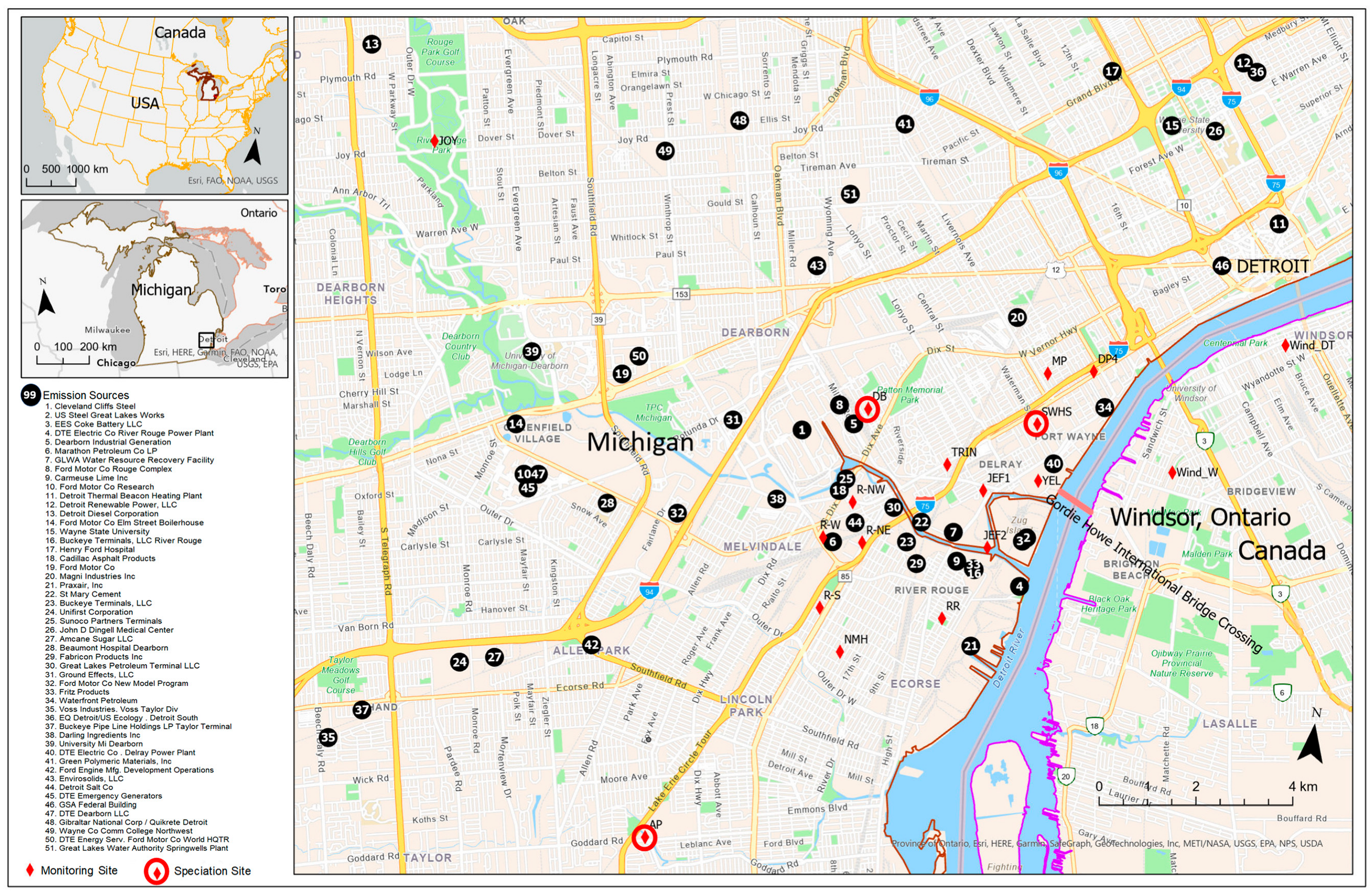
2.1. Study Area and Monitoring Sites

Detroit is a US Midwestern city with a population of 660,000 located in the 9-county Detroit–Ann Arbor–Flint Combined Statistical Area (CSA) that has a population of 5,428,000 persons [29]. Detroit’s many residential neighborhoods are interspersed among heavy and light industry, e.g., vehicle manufacturing, steel and coke production, petroleum refining, cement and asphalt plants, water and wastewater treatment, power plants, recycling and waste treatment/disposal, truck and train traffic, intermodal and logistics facilities, commercial activities, and extensive construction/demolition activities, including a major new international bridge crossing. The 2019 Michigan Air Emission Reporting System (MAERS) lists 328 facilities reporting air emissions within 50 km of the study area (for facilities emitting > 1 ton/year of conventional pollutants plus methane). Collectively, these sources emit 2148, 16,137, and 18,150 tons/year of PM, SO2, and NOx, respectively; considering sources within 5 km, 76 facilities emit 904, 7784, and 6765 tons/year, respectively, based on 2019 data. Historically, emissions were much higher, even as recently as 2000 or 2010. Figure 1 shows locations of major point sources, the largest of which include two steel plants and a coke battery. Major sources that have been shuttered in recent years include the 358 MW(e) DTE River Rouge power plant that was phased out from 2002 through 2016 by switching from coal to natural gas until retirement in 2021 (2010–2014 emissions averaged 25, 10,443, and 3416 tons/year for PM, SO2, and NOx, respectively); the 550 MW(e) DTE Trenton Channel power plant, another coal-fired unit that reduced emissions over the 2013–2016 period and which was scheduled to be retired in 2022 (2010–2014 emissions averaged 646, 20,824, and 4409 tons/year for the three pollutants, respectively); and the Greater Detroit Resource Recovery Authority waste incinerator (4000 ton/day capacity) that closed in early 2019 (2010–2014 emissions averaged 22, 141, and 1162 tons/year, respectively). Other major sources that shut down earlier include the Mistersky Power Plant (2004, 154 MW(e), oil, gas); the Conners Creek Power Plant (1988, 240 MW(e), coal, gas); and the Wyandotte Municipal Power Plant (73 MW(e), 2017, coal, gas, tire-derived fuel). Reduced emissions of SO2 and NOx from other sources in the region and nationally have furthered lower levels of secondary sulfate and nitrate.
Southwest Detroit’s air quality monitoring network is mapped in Figure 1. Three monitoring sites were selected due to their proximity, the PM2.5 components measured, the completeness of the monitoring record, and the diversity of nearby sources. The Allen Park (AP) monitor is ~8 km southwest and often upwind of Detroit’s main industrial area. The site is located in a small city (18.1 km2; population of 28,237) [29]) that has some manufacturing activity [30]. The monitor (AQS ID: 26-163-0001; lat/long: 42.228611/−83.20833) is designated as a “population-oriented” site and is 190 m southwest of interstate highway I-75 that has moderately high vehicle volume (86,099 vehicles/day, annual average daily traffic, AADT) and high truck volume (16,476 vehicles/day, commercial annual average daily traffic, CAADT) [31]. The monitor is in a small field near some forested land, several enclosed wastewater tanks, and light commercial and trucking facilities. Data from this site have been used to assess mobile source contributions [32].
The Dearborn (DB) monitor, 9.9 km northeast of AP site, is designated a “maximum concentration” site (AQS ID: 26-163-0033; lat/long: 42.306674/−83.148754). Adjacent to Detroit, Dearborn is a densely populated city (62.8 km2; population of 108,420) [29] with considerable industrial and commercial activity. The monitoring site lies between highways I-94 (1.85 km to the north; AADT and CAADT of 92,030 and 12,215 vehicles/day, respectively) and I-75 (2.3 km to the southeast; 86,099 and 16,476 vehicles/day) [31]. Major industry within 1 km includes automobile assembly (Ford), steel and coke production (Cleveland Cliffs and River Rouge Complex), coal- and gas-fired electric utilities, and the Detroit wastewater treatment facility (which includes multiple sludge dryers and incinerators); industry within 2.5 km includes a refinery, cement and asphalt plants, and many logistics facilities. A salt mine ([33], Figure 1) is ~2 km from the site, along with materials handling facilities, metal processors and recyclers, and other industries.
The third site, called Southwestern High School (SWHS; AQS ID: 26-163-0015; lat/long: 42.302786/−83.10653), is 3.6 km east of DB and also is a “maximum concentration” site. The site is 245 m south of Fort Street (7436 and 1121 vehicles/day, AADT and CAADT, respectively), 0.2 km south of M-85 (7436 and 1109 vehicles/day), and 0.3 km south of I-75 [31]. Notably, the site is adjacent to a very large construction area that will become the inspection and customs terminal for the new Gordie Howe International Bridge (construction phase from 2018–2024). This site recorded the highest SO2 concentration in the area, leading to the area’s designation as non-attainment for the SO2 National Ambient Air Quality Standard.

2.2. Sample Collection and Data Cleaning

PM2.5 samples for chemical speciation were collected every third day at AP and every sixth day at DB and SWHS. We focus on a 6-year period from 1 January 2016 to 31 December 2021. Following protocols in the Speciation Trends Network [34], Met One SASS and URG samplers were used to collect filter samples, which were analyzed for elements using X-ray fluorescence on Teflon filters, ions by ion chromatography on nylon filters, and elemental (EC) and organic carbon (OC) by thermal optical transmittance (TOT) on quartz filters. We also obtained PM2.5 measurements using two Federal Reference Methods (FRM). Data were obtained from US EPA and the Michigan Department of the Environment, Great Lakes and Energy (EGLE).
Several steps were used to clean and impute data. We checked for reasonable ranges and possible outliers of each parameter by examining the highest values. As described in the Supplemental Materials (SM), some missing Na+ data were imputed, and a small number of observations were considered outliers or possibly erroneous and were removed. The number of daily observations in the final dataset was 693, 353, and 347 at AP, DB, and SWHS, respectively.

2.3. Descriptive Analyses

Descriptive statistics were calculated for each parameter for the full study period as well as stratified by season (winter as December to February; spring as March to May; summer as June to August; fall as September to November) and calendar year for selected pollutants. Seasonal trends were displayed using 3-month running averages. Trends over the study period, differences in concentrations between the three sites, and differences between before and during the pandemic lockdown were examined by comparing full-year periods (19 March 2019–19 March 2020; 20 March 2020 to 20 March 2021) to avoid seasonal effects. The analyses used density plots and t- and Mann–Whitney U tests given the nonnormality of the data (based on Shapiro–Wilk normality tests). Additional descriptive statistics and analyses are in the Supplementary Materials (Table S2, Figures S2–S4).

2.4. Positive Matrix Factorization

PM2.5 at the three sites was apportioned using positive matrix factorization (PMF), which identifies and quantifies contributions of sources based on the chemical composition of sources and ambient monitoring data. US EPA PMF version 5.0 [35,36] was used with parameters and procedures that followed recent literature [26,28,37,38,39]. The SI describes both PMF and the procedures. Modeling used two approaches. The first and “conventional” approach developed separate PMF models for the 6-year record at each site. The second approach consolidated data across the three sites, developed a single set of source profiles that applied to the three sites, and estimated all factor loadings in a single analysis. Otherwise, parameters and data treatment were similar to the first approach. To implement this approach, dates for the second and third sites were displaced by 5 and 10 years, respectively (thus obtaining a unique date for each observation), the three datasets (one per site) were concatenated (allowing the PMF program to run without modification), PMF models were estimated, and then the correct dates were restored. This approach, called approach 2, is motivated by three potential advantages: it incorporates both temporal (across the 6 years) and spatial variation (across the 3 sites) in pollutant levels; the derived profiles apply to all sites and thus should facilitate comparisons across sites; and the larger sample size should increase robustness. The method has two potential disadvantages. First, factor profiles might vary spatially and change over time; however, nearby sites likely have similar conditions and the model should be able to handle some variation. Second, a source factor that is unique to one location might erroneously obtain a non-zero contribution at another location since source contributions are estimated for all factors at all sites. These concerns were evaluated by contrasting results for the two approaches.
In both approaches, the number of factors selected was guided by the literature and separation of source types. PMF models with 6 to 10 factors were tested, and the final selection was based on the clearest interpretation of sources. The 7-factor models were most informative. Models with fewer factors were difficult to interpret as species were often shared between factors, while models with more factors often split similar sources into several profiles. The seven factors were classified as follows: secondary sulfate, including SO42−, S, and NH4+; secondary nitrate with NH4+ and NO3; vehicles/mobile sources with EC and OC, for which EC tends to denote diesel particulate matter from pyrolysis [32,40,41] and OC reflects combustion products from gasoline vehicles and other fossil fuels, biofuels, and open burning [32,42]; iron/ferrous metals (Fe, Zn); salt with Na+ and Cl; soil/crustal material (Al, Ca, Si); and non-ferrous metals industry with Cu and other metals. In some 8-factor models, a combination of elemental sulfur with crustal/dust elements suggested a mixture of soil/dust and deposited sulfate that was subsequently suspended from unpaved roads [14,43].
Apportionments comparing pre-pandemic and pandemic periods were estimated using PMF models with three approaches: approach 1 used two PMF models at each site, one for each period; approach 2A used a single model that combined the two periods and the three sites; and approach 3 used an individual model at each site that combined the two periods. These approaches have different strengths and weaknesses; e.g., approach 1 allows the greatest flexibility but results may not be comparable if profiles change; approach 2A is similar to approach 2 described earlier that used a longer duration (6-year period); and approach 3 facilitates comparisons between time periods but not sites. In each case, predicted normalized daily factor contributions from the PMF model (mean contribution of each factor is 1) were multiplied by the factor profiles to obtain daily predictions of PM2.5 and potential source contributions [39,44,45]. Seasonal apportionments were calculated as the average of daily predictions in the season; this was also confirmed using PMF models developed for that season. The seasonal variation was displayed using trend plots and 3-month running averages calculated using daily predictions of source contributions from the PMF models.

3. Results

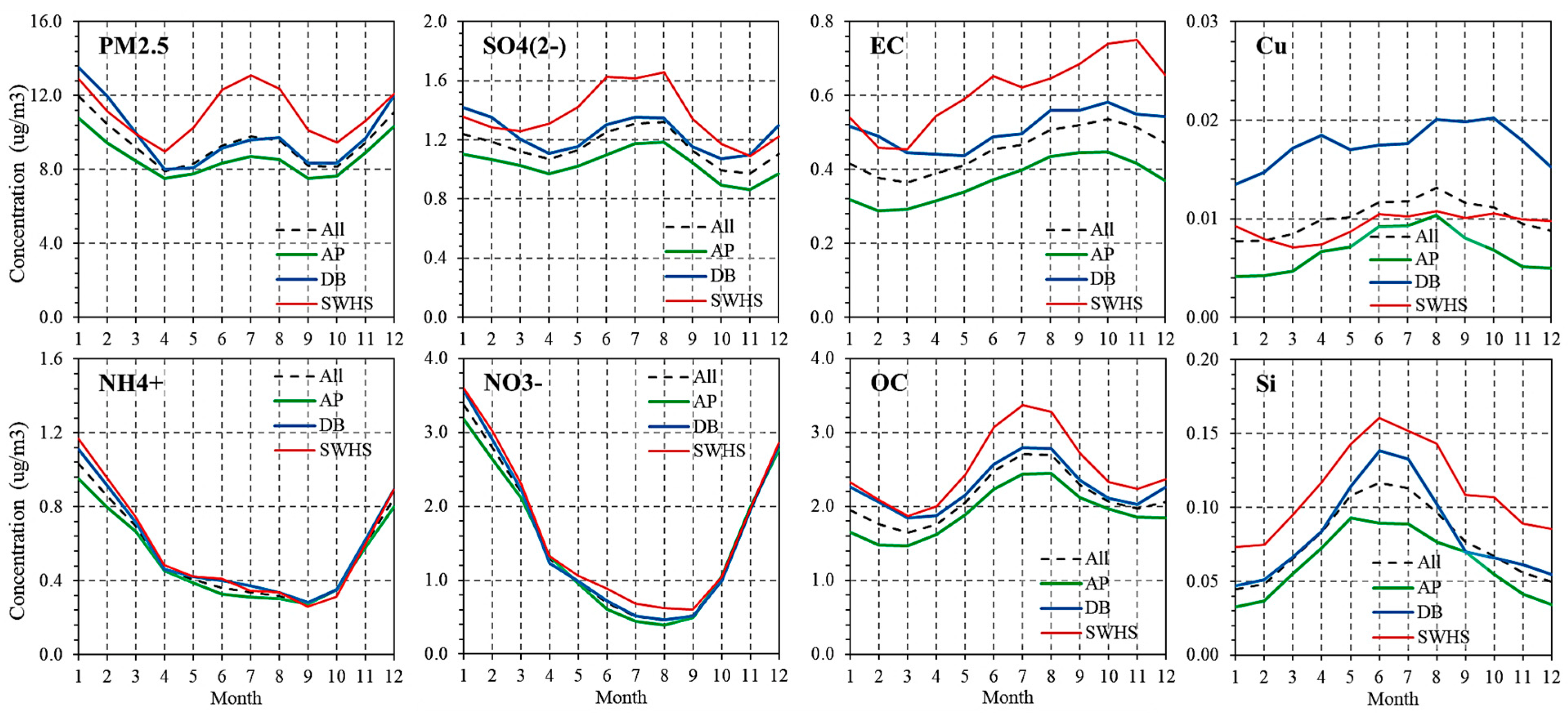
3.1. Summary, Seasonal, and Annual Trends

Summary statistics for key variables (PM2.5, NH4+, NO3, SO42−, S, EC, and OC) at the three sites are shown in Table 1; statistics for other species are in Table S2. Over the study period, 24 h PM2.5 levels (± standard deviation) averaged 8.6 ± 4.8, 9.9 ± 5.4, and 10.8 ± 5.5 µg/m3 at the AP, DB, and SWHS sites, respectively (N = 693, 353, and 347). In addition to having the highest PM2.5 level, the SWHS site had the highest levels of NH4+, NO3, SO42−, S, EC, and OC; DB had intermediate levels; and AP had the lowest levels. Differences between the ‘low’ AP site and the two other sites were statistically significant for most of these species except NO3 in the AP–DB comparisons and NH4+ in the AP–SWHS comparisons (Table S3). Only small differences or gradients in concentrations in the area are expected for secondary pollutants such as SO42− that arise from mostly distant sources (e.g., the many power plants in the Ohio River Valley); local emissions may cause the variation observed.
Over the 6-year study period, annual average levels of PM2.5 varied about 10% (coefficient of variation), and the levels in 2020 fell by 0.9 and 1.4 µg/m3 from 2019 levels at the AP and SWHS sites, respectively (Table 2), suggesting a pandemic-related effect of the lockdown (examined in Section 3.4). Several pollutants showed strong seasonal variation (Figure 2). PM2.5 levels at the three sites were bimodal, with winter and summer peaks, especially at SWHS, which has had some of the highest PM2.5 levels in Michigan in recent years, potentially reflecting industry, fugitive dust, and construction activity. NH4+ and NO3 peaked in winter, while Si, Al, and other crustal elements peaked in summer, likely reflecting entrained soil and dust. OC trends were bimodal and similar to PM2.5. Other species with systematic but less pronounced variation included EC (highest in fall); SO42− and S (highest in summer) [15]; and SO42− (small winter peak). In addition, Cu showed a summer peak at AP, although DB had considerably higher Cu levels without much seasonality, suggesting the influence of different sources at these sites.

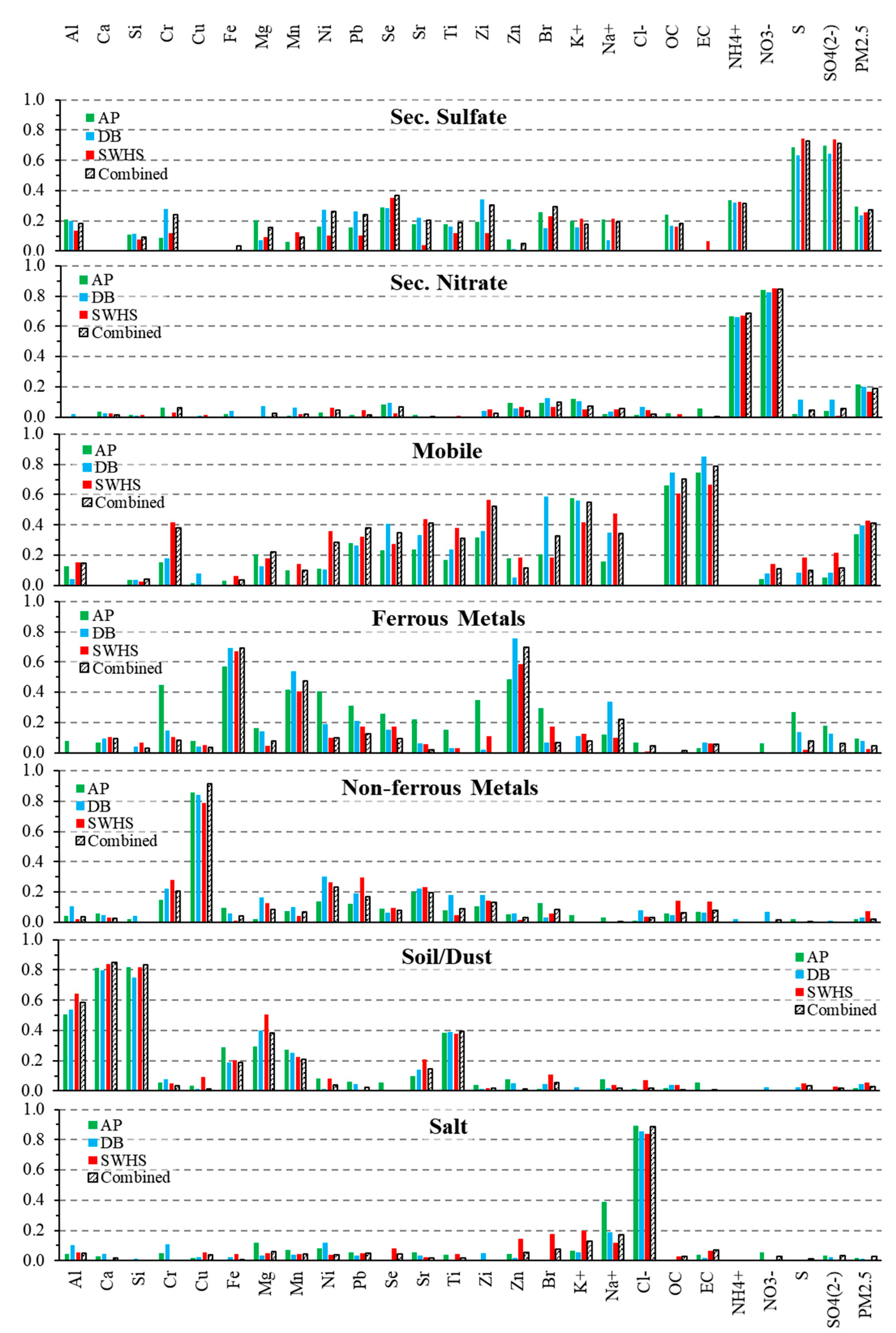
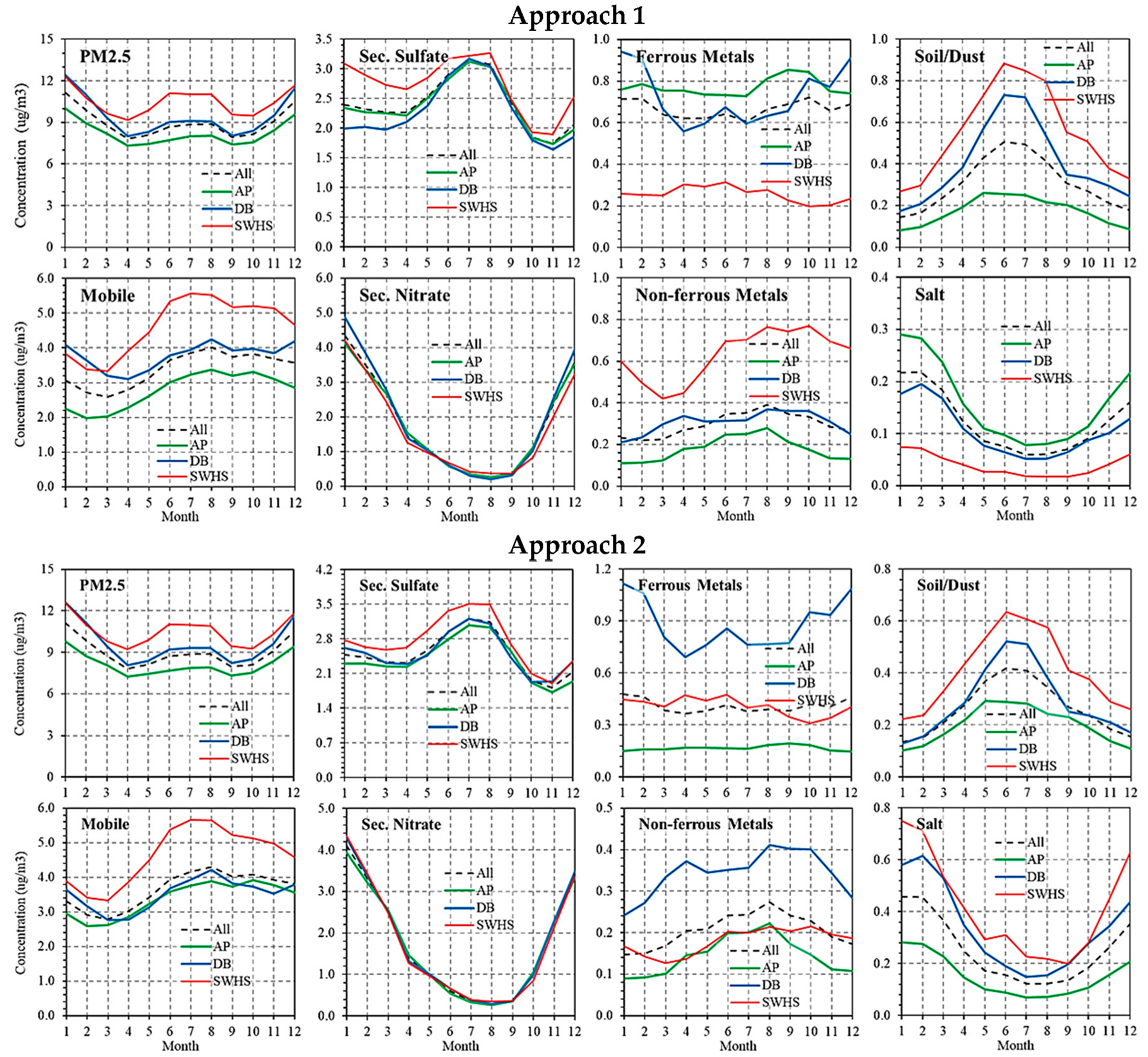
3.2. Comparison of Profiles and PMF Approaches

Differences among the profiles for the PMF models are shown in Figure 3, which displays four sets of profiles for the seven source types: three sets are from the PMF models analyzing AP, DB, and SWHS sites separately (approach 1); and the fourth set is from the consolidated dataset (approach 2). In some cases, small differences in profiles can affect apportionment results. The following discusses differences among the profiles and compares them to literature profiles (84 literature profiles are tabulated in Table S5). Literature- and PMF-derived profiles may not match due to local conditions, the reactivity of species, and gaps and issues of representativeness in the available profiles. This particularly applies to heavy-duty diesel vehicle exhaust and nonroad gasoline exhaust sources [46] that are highly relevant for Detroit.
Secondary sulfate and nitrate had similar profiles across the three sites. The secondary sulfate profile was dominated by SO42−, S, and NH4+; some OC was included, as observed in other PMF studies [27,38,46,47], likely reflecting organic matter in polluted urban air that condenses on sulfate particles [27] and possibly low-volatility organic matter formed in acidic particle environments [48]. Secondary nitrate had a simple profile, characterized by NH4+ and NO3. Nitrate precursors include ammonia (NH3) from animal feeding, fertilizer use [49] and some industrial processes [50], and nitrogen oxides (NOx) from mobile sources, power generation, industry, and other combustion sources [51]. Mobile source profiles were dominated by EC, OC, and K+; the SWHS profile had more S, SO42−, Zn, Cr, and Ni than the other two sites. Literature profiles relevant to mobile source exhaust emissions contain considerable EC, OC, and other species but little K+, which is typically a marker for waste or wood combustion, some metals industries (e.g., sintering furnaces), cement, and road dust. This suggests that the mobile contribution at SWHS included both exhaust emissions as well as some suspended road and cement dust, which is consistent with the highway and bridge construction activities described earlier. In addition, this site is near the Detroit River and the Port of Detroit and possibly affected by ship and train emissions. The salt profiles were similar and simple, consisting of Na+ and Cl, with some Mg; the profiles differed in amount of Na+ and some trace metals.
The ferrous and non-ferrous metals profiles showed the greatest differences among sites and approaches. Ferrous profiles were dominated by Fe and Zn, with smaller levels of Mn and other metals. Other species in the profile varied by site: AP included high levels of Cr, Ni, and Zi; DB and SWHS sites (and approach 2) were generally similar. Fe arises from iron smelting and steel manufacturing. Zn has many of the same as well as additional sources, e.g., municipal incinerators [51,52,53]. Given the distance between AP and local metal industries, the AP profile likely represents a mixture of ferrous industries and some entrained soil and dust. Literature profiles for the ferrous industries are diverse: profiles for furnaces, steel desulfurization, shredding, and heat-treating show Fe; many show K, Cl, Mg, S, SO42−, OC, and EC; and some show crustal elements Ca and Ca (but little Si) [52]. Profiles for non-ferrous metals were dominated by Cu, with smaller contributions from other metals (e.g., Cr, Ni, Pb). The SWHS profile included higher levels of Pb compared to the other sites, possibly reflecting soil entrainment and demolition activities. Profiles developed in approach 2 maintained these metals but had smaller contributions. Similarly, nonferrous profiles in the literature are diverse and include processing and production of different metals. The Detroit profiles appear consistent with profiles for Cu and perhaps Pb processing. Most of the literature profiles for nonferrous metals also include Cl, S, SO42−, Si, and Zn, and some included Na.

3.3. Long-Term and Seasonal Apportionments

The estimated long-term apportionments from the two PMF approaches are listed in Table 3. Orange shading in the table highlights an apportionment at a site that exceeds 25% of the average apportionment across the three sites; blue shading represents a 25% decrease from the average. Such changes were observed for several of the local sources categories, e.g., mobile, ferrous metals, and non-ferrous metals. The other source categories, i.e., secondary nitrate and sulfate, soil/dust, and salt, showed only small differences from the three-site mean. This suggests the importance of spatial variability for local industrial and mobile sources, i.e., monitor placement can significantly affect apportionments.
Figure 4 shows seasonal trends of the apportionments, which generally follow patterns of the pollutant levels observed earlier (Figure 2), e.g., winter peaks for secondary nitrate and salt and summer peaks for secondary sulfate, soil/dust, and mobile sources. These patterns, some of which have been described previously [15,27,54], reflect climatic influences on pollutant formation, use of salt for deicing roads in winter, and seasonal shifts in meteorology and prevailing winds, e.g., the prevailing winds arise from the SW except in spring, when winds from most sectors have similar likelihood. (Figures S12–S13 show annual and seasonal wind roses.) The non-ferrous metals factor shows yet another pattern, peaking in the summer or fall, potentially representing entrained dust from metal processing facilities. The other source factors had less seasonal variation.
Mobile sources were the largest single contributor to PM2.5 levels at each site, accounting for 2.8–4.3 µg/m3 (34–42%) of PM2.5 depending on site and PMF approach. The estimated contribution was highest at SWHS, which is relatively close to an arterial road and a major (I-75) highway. However, the large GHIB construction site and associated non-road sources may dominate mobile source contributions at this site, which is supported by seasonal trends that show the highest contributions during the summer/fall construction season (Figure 4). Starting in 2018 (Michigan side only), this 6-year $5.7 billion project entailed widening and reconstruction of 3 km of I-75 with nine new bridges, ramps, and service lanes, and, at the bridge/terminal site itself, demolition, grubbing, clearing, backfill, installation of 105,000 wick drains (20 m depth), fill placement (over 1 million cubic yards), installation of foundation shafts, and extensive aboveground work, including construction of 2.5 km of main roads, the 68 hectare port of entry facility (with a 30,318 m2 terminal/customs building), 36 primary inspection lanes, and the cable-stayed bridge spanning 853 m (https://www.gordiehoweinternationalbridge.com/en/project-overview, accessed on 16 December 2022). Similar activities commenced in 2015 on the Canadian side of the Detroit River, 2 km SE of the SWHS site. These activities are performed using diesel-powered vehicles and equipment and entail considerable earth moving, concrete cutting, and other sources of fugitive emissions.
Levels of secondary nitrate and sulfate were similar at the three sites, jointly contributing 4.2–4.4 µg/m3 (43–51%) of PM2.5. The two PMF approaches yielded similar results for these pollutants. As noted, distant sources likely contributed most of the sulfate, with nearby SO2 sources causing local variation; the small SO42− gradient observed (e.g., average of 0.3 µg/m3 higher at SWHS compared to AP) follows the SO2 concentration trend. Notably, nearly all the local coal-fired facilities operated without scrubbers. While these facilities are being scaled back, retired, or replaced with gas turbines, when operating, plumes from these sources would likely reach the nearby monitors too quickly for much conversion of SO2 to SO42−. There are many other coal facilities in Michigan, the Ohio River Valley [25], and further afield in Indiana and Pennsylvania that have sizable SO2 emissions and likely cause most of the sulfate in the region [55], although their emissions also have been declining in recent years.
Apportionments for the other source categories showed several differences between the two PMF approaches (Table 3). Based on the separate models (approach 1), ferrous metals contributed 0.72–0.77 µg/m3 at AP and DB but only 0.22 µg/m3 at SWHS; approach 2 provided the highest contribution at DB (0.88 µg/m3) and the lowest at AP (0.17 µg/m3). The results from approach 2 are consistent with known sources, e.g., the DB site is 0.5 km ENE and typically downwind of the large Cleveland Cliffs steel complex (source 1 in Figure 1). The area has many other steel and ferrous metal processing industries. The SWHS site is 1.55 km NNE of the Zug Island complex, the area’s second largest steel mill (US Steel/National Steel, source 2 on Figure 1); however, its activity and emissions have been considerably curtailed since 2010. (Tables S6–S8 show emission rates at major sources in the region). The AP site, which had the lowest ferrous metals contribution, is 8.1–9.5 km SE and generally upwind of these sources. While now shuttered, ferrous industries had operated further south and closer to AP, a possible reason why the composition of entrained soil and dust may resemble the ferrous metals profile, although entrained materials tend to be particles larger than PM2.5.
For non-ferrous metals sources, approach 1 provided a relatively large contribution at SWHS (0.75 µg/m3) that peaked in summer and fall, but low levels elsewhere (<0.17 µg/m3); approach 2 provided DB the highest contribution (0.34 µg/m3) and small contributions elsewhere (<0.18 µg/m3), with some increases in summer and fall. Again, approach 2 was consistent with locations of known industries. There are many potential sources of Cu, e.g., smelting and roasting of copper, lead and other metals (not in Detroit in recent years), nonferrous and secondary metals processing and recycling, oil refining, sintering furnaces, vehicle tire and brake wear, sewage sludge incineration, and iron casting [51,56]. Another possible source is brush wear on electric motors, including those used in air sampling [57]. More sensitive measurements that include additional elements might help separate these sources; e.g., Sb typically accompanies Cu when associated with tire and brake wear.
For salt, apportionments also depended on the approach, although the predicted contributions were small. Approach 1 had the highest contribution (0.16 µg/m3) at AP; approach 2 increased predictions at DB and SWHS to 0.34 and 0.43 µg/m3, respectively. All three sites showed strong and similar seasonal patterns consistent with aerosolized salt from road deicing, i.e., peaks in mid- and late winter [27], which would not be expected from ocean-derived aerosols at this inland location.
The highest soil/dust contributions were found at SWHS, adjacent to the large construction area for the international bridge; even so, the levels were modest (<0.75 µg/m3). This factor was dominated by crustal elements Ca, Si, and Al, with smaller amounts of Fe, Mg, Mn, and Ti, which can represent several sources, primarily soil (mostly local but occasionally regional or intercontinental) and dust, and possibly vehicle-related emissions, e.g., exhaust and brake and tire wear [27,46]. The area contains many materials handling facilities that store, process, and transport scrap metal, aggregates, cement, salt, and other commodities. Siltation and wind- and truck-entrained dust are frequently observed near these facilities, but these are mostly larger particles not expected to contribute to PM2.5.
In summary, the two PMF approaches provided similar seasonal trends and comparable apportionments when averaged across the three sites (Table 3). However, on a site-to-site basis, the results differed for several factors, most notably for ferrous and non-ferrous metals, soil/dust, and salt. Apportionments obtained using approach 2 were more consistent with the proximity of the monitoring sites to known local sources. Overall, the comparison suggests that the results obtained for the consolidated datasets in approach 2 are easier to evaluate and more consistent than the results of separate models for each site.

3.4. Changes during the Pandemic

Only a few of the pollutants across the three sites showed statistically significant changes in mean or median levels between 1-year periods before and during the pandemic (Table S4). Changes in PM2.5 levels were small and none approached statistical significance. One change common across the three sites was a decrease in median EC levels during the pandemic (Mann–Whitney tests, p ≤ 0.05); however, changes in means were modest and generally not statistically significant, and black carbon, a closely related pollutant, did not change (except at AP). A richer although qualitative interpretation of changes is shown by the monthly trends and density plots for the two periods (Figures S2–S7, respectively), as well as the PMF apportionments for the two periods, which are summarized in Table 4 and discussed below. The SI discusses additional changes in the pollutant levels and PMF results and presents the PMF profiles for each approach (Figures S8–S11).
During the pandemic, mobile source contributions decreased slightly at AP and DB and more substantially at SWHS (based on approaches 2A and 3), possibly reflecting the slowdown from on-road and non-road mobile sources (e.g., train, ship, construction equipment) associated with local commercial, industrial, and transport sectors, including intermodal, port, and logistics centers. However, mobile contributions during the 2-year period (approaches 2A and 3) remained similar to those estimated for the 6-year period (approach 2, Table 3). The drop in mobile source contributions at SWHS may reflect a slowdown in construction activity at the bridge site. Secondary nitrate showed little change over the 2 years, although levels increased by 9–20% compared to the 6-year analysis (comparing methods 2 and 2A). Secondary sulfate increased at DB (approaches 2A and 3), although levels at the three sites were 34–37% lower than the 6-year results, reflecting the continuing long-term decline in SO2 emissions. The mostly small changes in secondary pollutants over the 2-year period suggest that emissions from many local and regional sources (e.g., power plants) remained unchanged, at least during the earlier phase of the pandemic, or that changes were indistinguishable given meteorological variability. In contrast, the smaller and local sources showed relatively large changes. Contributions from ferrous metals decreased at all sites and for all approaches, and contributions were 23–49% lower than in the 6-year analysis. This pattern suggests a short-term slowdown in industrial and manufacturing activity in addition to the long-term downward trend. Nonferrous metals decreased at AP and DB but increased at SWHS. Similarly, soil/dust decreased at AP and DB (except for approach 1) but increased at SWHS. The soil/dust increase at SWHS likely reflects extensive construction activity along I-75 in 2020.
The apportionments showed some differences by site and PMF approach, as expected. Approach 1 yielded apportionments for the smaller sources (e.g., ferrous metals) that fluctuated widely between pre-pandemic and pandemic periods, and differences from 6-year results (Table 3) were sometimes large. This approach used a single year of data in each model and the composition of some profiles shifted, although the main species for each factor remained constant. Generally, smaller changes occurred at AP, which had twice the number of samples (due to AP’s 1-in-3 day sampling schedule compared to 1-in-6 elsewhere). Together, these observations suggest that larger sample sizes are needed to reduce statistical variability. The results show several other patterns. Approaches 2A and 3 provided similar results and yielded apportionments for pre-pandemic and pandemic years that had small to moderate differences; this consistency may reflect the design of these approaches, which was intended to examine temporal changes. Most of the apportionments show that contributions from mobile sources at SWHS and from ferrous metal and nonferrous metals sources at all three sites diminished during the pandemic; these changes appear to reflect actual pandemic-induced effects, although fluctuations due to meteorological variability cannot entirely be ruled out. While effects might be sensitive to the data subset and other factors, most changes were small and PM2.5 levels remained unchanged.
Many studies have considered changes in pollutant levels associated with the pandemic lockdown, and a review of 114 studies broadly suggested that PM2.5 and NO2 levels tended to decrease during the lockdown period, especially in polluted areas in Asia, while O3 levels tended to increase; changes in SO42− and CO were more variable [58]. Our analysis in southwest Detroit shows several changes in source contributions to PM2.5 but no significant change in the average (or median) PM2.5 concentration. We also show that such assessments should account for both short- and long-term changes (including seasonal variation), use robust methods, and recognize that trends might differ locally within a region or for portions of the pandemic period.

4. Discussion

4.1. Comparison to the Literature

PM2.5 apportionments in the Detroit area over the past 20+ years are summarized in Table 5. (The table omits studies with very short duration, e.g., [59].) Because PM2.5 levels have been declining, contributions from different sources are discussed in terms of concentrations (not relative fractions or percentages) to avoid a shifting baseline. Where possible, concentrations were derived from the cited studies.
We found that mobile sources, which contributed an estimated 2.76–4.31 µg/m3 (34 to 42% of PM2.5), represent the largest single contributor at the three sites. The mobile source profiles emphasized EC and OC, although some K+ was included, which has been associated with biomass combustion ([25]; Table S5). The seasonal variation in EC and OC levels was modest (Figure 2), as noted earlier [27,54], and somewhat moderated in the mobile source plot (Figure 4). Several earlier studies in Detroit have obtained comparable results, identifying specific mobile sources, e.g., highways [16], truck, rail, and ship traffic at the Port of Detroit, and traffic on the Ambassador Bridge near the DB and SWHS sites [27]. Extensive on-road vehicular and train traffic has been observed near the DB site, including throughout the night [17], and heavy-duty diesel traffic at the bridge and nearby arterials and residential streets is common, in part due to road closures associated with construction activity. The most recent prior apportionment in Detroit used 2001–2014 data from the AP monitor and a nine-factor PMF model to estimate vehicle contributions of 2.02 µg/m3 (21% of PM2.5) [28]. The lowest estimate of vehicle contributions, 1.27 µg/m3, used 2007 DB data and a 10-factor PMF model [17]; the large number of factors may have decreased the contribution. The highest estimate, 6.40 µg/m3, used 1999–2002 data at a residential neighborhood 0.38 km NNE of I-75 near an arterial with regular truck traffic (lat/long: 42.31656/−83.09365) and a seven-factor model [25]. Because this analysis did not include nitrate, secondary nitrate may have been assigned to vehicles; further, the soil/dust/crustal estimate was small and again possibly transferred to vehicles. The mobile source profiles in the earlier studies differed by inclusion of K+, Al, Cu, Fe, and Pb, which can increase the estimated contribution due to dust and soil entrainment. While our profile included some K+ (except at SWHS in the separate models), we maintained a separate soil/dust profile. Notably, the four studies that separated diesel and gasoline vehicles showed large PM2.5 contributions from gasoline vehicles; e.g., diesel and gasoline vehicles contributed 2.16 and 4.24 µg/m3, respectively, in a seven-factor model using 1999–2002 data from SW Detroit [25], the highest estimate for gasoline vehicles among studies that separated vehicle types. Lower estimates were obtained at AP, 0.67 and 2.53 µg/m3 for diesel and gasoline vehicles, respectively, using an eight-factor PMF model and 2000–2005 data [27].
We found that secondary sulfate was the second most important source of PM2.5, contributing 2.27–2.67 µg/m3. Literature estimates for this pollutant vary widely, from 3.17 to 11.00 µg/m3. Notably, all of these estimates exceed those in the present study. The lowest contribution was estimated at AP using a nine-factor PMF model and 2001 to 2014 data [28]; the highest was at Eastside Detroit using a five-factor PMF model and 1999 to 2002 data [25]; this analysis that did not include species that contribute to secondary nitrate, e.g., NH4+ and NO3, which likely inflated the sulfate estimate.
Prior estimates of secondary nitrate contributions also have ranged widely, from 1.61 to 4.49 µg/m3. The lowest was at DB using a 10-factor PMF model and 2007 data [17]. Using AP data, Milando et al. [28] obtained results similar to the present study. Three studies using older data (2000–2006) reported high contributions (3.89–4.49 µg/m3). Our results reflect a nearly 50% decrease in measured nitrate levels over the past two decades; e.g., nitrate at AP averaged 2.67 and 3.21 µg/m3 in 2002 and 2004 but only 1.61 and 1.43 µg/m3 in 2019 and 2020.
The ferrous metals contribution at DB was 0.88 µg/m3, considerably higher than at SWHS and AP (approach 2). Notably, all prior studies in Detroit identified a ferrous (or “metals”) source, with a large range of contributions (0.02–3.63 µg/m3). Non-ferrous metals contributions ranged from 0.15 to 0.34 µg/m3 (approach 2), spanning the 0.29 µg/m3 estimated at AP using a nine-factor model and 2001–2014 data [28]. No other prior study in Detroit separated non-ferrous metals; rather, they were combined with Fe in a broader “metals” category.
We estimated only small contributions from salt, <0.28 µg/m3 (approach 2). Levels in earlier studies span our results, ranging from 0.19 µg/m3 from a 10-factor PMF model using 2007 data [17] to 0.72 µg/m3 from an eight-factor PMF model using 2000–2005 data [27]. Earlier studies also reported a wide range of soil/dust contributions, ranging from a low of 0.02 µg/m3 estimated using a seven-factor PMF model, 1999–2002 data, and La, Ce, and P as tracers (Si and Ca were not included in this analysis) [25] to a high of 2.14 µg/m3 using an eight-factor model and 2000–2005 data [27]. The profile for the latter estimate was likely inflated as it included significant levels of Fe, EC, and S, which we attributed to other sources (mainly ferrous metals and mobile sources).

4.2. Emissions Inventories

State and national emission inventories have reported substantial reductions in many pollutants in recent decades, as shown in Table 6 for Wayne County, which encompasses Detroit. (Tables S6–S8 list emissions for the 50 largest facilities in the county.) As noted earlier, different inventories may not be fully comparable, and comparisons between years can reflect changes in methodology. Over the past 20 years, SO2 and NOx emissions from mobile and stationary sources have been cut dramatically; longer-term trends show yet larger reductions (Figure S14). PM2.5 and PM10 trends are complex and have more uncertainty. For mobile sources, the NEI shows large reductions in PM2.5 and PM10 from 2000 to 2017. This applies to both on-road and non-road emissions, which have roughly comparable emission rates in Detroit. Stationary sources in MAERS show seven- and three-fold reductions from 2000 to 2010 in PM2.5 and PM10 emissions, respectively, followed by modest increases in PM2.5 emissions; PM10 emissions stay largely unchanged. The PM2.5 increase in MAERS reflects greater emissions at coke and steel facilities. (The other NEI source categories do not show these changes.) The largest PM2.5 emission sources in the 2017 NEI include natural gas (1007 tons/year in Wayne County), miscellaneous non-industrial (741 tons/year), commercial cooking (645 tons/year), mining (467 tons/year), wood (471 tons/year), ferrous metals (392 tons/year), paved road dust (335 tons/year), construction dust (212 tons/year), petroleum refinery (84 tons/year), and waste disposal (84 tons/year).
The emission inventory information suggests potentially important source categories for apportionments. The PMF models reflected the significance of emissions from mobile sources, ferrous (steel and coke) metals, soils/dust (construction, paved road, unpaved road), and other sources; however, we could not distinguish incinerator, refinery, cooking, wood, and several other categories. At the same time, limitations of inventories should be recognized: they do not account for pollutant dispersion and fate, formation of secondary pollutants, and regional pollutant sources. Further, mobile and nonpoint emissions are determined at a county level, and uncertainties can be large, especially for PM. Inventories are updated only periodically. For these reasons, we saw little correlation between annual changes in inventories and monitoring data.
The PMF results highlight the importance of secondary sulfate and nitrate, pollutants that form from both local and regional emissions of SO2 and NO2 precursors at rates that depend on levels of oxidants, insolation, ammonia, temperature, humidity, and other factors. Secondary particulate carbon can also form from reactive organic gases emitted by mobile and stationary sources, forest fires, and biogenic sources. Levels of secondary pollutants resulting from local precursor emissions can be estimated using chemical transport modeling as well as older and simpler methods, e.g., Modeled Emission Rates for Precursors (MERPs, essentially a ratio of local to regional emissions of precursors [60]) and offset ratios representing a fraction of precursor emissions for use in dispersion models to estimate PM2.5 (e.g., 1 and 10% of the NOx and SO2 emission rates) [61]. These methods have application-specific parameters, conditions that preclude their use (e.g., complex terrain, proximity to large pollutant sources that impact atmospheric chemistry, complex meteorology) and sometimes large uncertainties. The variation in secondary nitrate and especially sulfate across the three sites (Table 1 and Table 3) suggests an impact from local sources. As suggested above, this impact could be obtained by conversion of only a small fraction of local SO2 and NOx emissions, which have been abundant in the study area.

4.3. Study Limitations

This study has several limitations. First, the three monitoring sites yielded some differences in trends and apportionments, particularly for smaller contributors (e.g., ferrous and non-ferrous metal industries), suggesting that additional sites may be needed to obtain results that are representative. Second, identification of sources and estimates of their contributions may be incomplete and uncertain for many reasons, e.g., not having unique or sufficient tracers for each source type, not identifying some sources, and possibly merging several types of sources in a factor. Incorporating more sensitive measurements, additional species and possibly size-specific information can help resolve sources [43]. PMF results can be sensitive to the number of factors, selected species, and data and time periods used. Some results were sensitive to the PMF approach and profiles, providing strong motivation for pooling data across sites and time periods. The daily data used may not capture short-term changes, especially from industrial sources [16]; this may also limit the ability to incorporate meteorological information that might help resolve some sources. Future work might utilize hybrid approaches, e.g., potential source contribution function (PSCF) and concentration weighted trajectory (CWT) models, to provide additional information regarding the location of potential sources that contribute to high air pollutant concentrations [62].

5. Conclusions

PM2.5 concentrations at three nearby sites in an urban and industrial area were apportioned to seven source classes using PMF models over a recent 6-year period and over 1-year periods to examine potential pandemic-related effects. The largest contributor to PM2.5 was mobile sources, which included both on-road vehicles and non-road sources, such as construction equipment. The next largest sources were secondary sulfate and nitrate, which have been declining over recent decades. Strong seasonal trends were observed for secondary nitrate, soil/dust, and road salt. While several pandemic-related impacts were suggested, e.g., reduced contributions from mobile sources at one site (SWHS) and reduced contribution from metal sources throughout the region, changes were small, possibly obscured by meteorological variability, and PM2.5 levels did not change significantly. PM2.5 contributions estimated for local sources depended on the location of the monitoring site, which indicates the importance of placing sites downwind of major sources as well as the need for multiple sites in Detroit and other large and complex airsheds in order to derive apportionments that reflect exposures in different areas. We found that apportionments derived using a PMF modeling approach that combined data across sites and time periods yielded results that were both more consistent and comparable, a result of incorporating both spatial and temporal variation, a larger sample size, and common profiles. No downsides to this approach were identified.
The long-term decline in levels of secondary sulfate and nitrate affects large swaths of the USA and potentially other countries, and suggests that apportionments of PM2.5 will increasingly reflect contributions from local sources, especially mobile sources, which have become the dominant source of PM2.5 in Detroit and likely in many other urban and industrial areas. This trend may increase site-to-site variability within an airshed, even as PM2.5 concentrations fall. In addition to the need to update apportionments, our analysis demonstrates that PMF models using pooled datasets can facilitate assessment of air quality trends and pollution sources.

Supplementary Materials

The following supporting information can be downloaded at: https://www.mdpi.com/article/10.3390/atmos14030592/s1: 1. PMF background; 2. Discussion of pandemic-related changes in pollutant levels, trends, and apportionments; 3. Supplemental figures and tables, including summary statistics, correlations, facility emissions, density plots, wind roses, PMF profiles, source profiles, and emission trends. References [8,26,27,37,38,39,62,63,64,65,66,67,68,69,70] are cited in Supplementary Materials.

Author Contributions

Conceptualization, S.B.; methodology, S.B.; software, Z.Y.; validation, S.B., Z.Y. and T.X.; formal analysis, Z.Y. and S.B., investigation, Z.Y.; resources, S.B.; data curation, Z.Y. and S.B.; writing—original draft preparation, Z.Y.; writing—review and editing, S.B. and T.X.; visualization, S.B. and M.K.I.; supervision, S.B.; project administration, S.B. All authors have read and agreed to the published version of the manuscript.

Funding

Funding supporting this research was obtained from the State of Michigan in grant 00E02952/AQDGG2020P2 provided by the US Environmental Protection Agency (EPA) entitled “The Southeast Michigan Chemical Source Signature (CHESS) Experiment”. Additional support was provided by grants P30ES017885 and R01ES032389 from the National Institute of Environmental Health Sciences, National Institutes of Health, and the City of Detroit/State of Michigan in a grant entitled “Air Monitoring for the Gordie Howe International Bridge.” The content is solely the responsibility of the authors and does not necessarily represent the official views of the sponsors.

Data Availability Statement

Data utilized in this study are freely available from the US Environmental Protection Agency and the Michigan Department of Environment, Great Lakes and Energy; specialized requests may also be directed to the corresponding author.

Acknowledgments

We acknowledge assistance of Eduardo Olaguer, Shelley Jeltema, Susan Kilmer, and Navnit Ghuman at the Michigan Department of Environment, Great Lakes and Energy.

Conflicts of Interest

The authors declare no conflict of interest.

References

  1. Hopke, P.K.; Croft, D.; Zhang, W.; Lin, S.; Masiol, M.; Squizzato, S.; Thurston, S.W.; van Wijngaarden, E.; Utell, M.J.; Rich, D.Q. Changes in the acute response of respiratory diseases to PM2.5 in New York State from 2005 to 2016. Sci. Total Environ. 2019, 677, 328–339. [Google Scholar] [CrossRef] [PubMed]
  2. Pun, V.C.; Kazemiparkouhi, F.; Manjourides, J.; Suh, H.H. Long-Term PM2.5 Exposure and Respiratory, Cancer, and Cardiovascular Mortality in Older US Adults. Am. J. Epidemiol. 2017, 186, 961–969. [Google Scholar] [CrossRef] [PubMed] [Green Version]
  3. Xing, Y.F.; Xu, Y.H.; Shi, M.-H.; Lian, Y.X. The impact of PM2.5 on the human respiratory system. J. Thorac. Dis. 2016, 8, E69–E74. [Google Scholar] [CrossRef] [PubMed]
  4. Yang, L.; Li, C.; Tang, X. The Impact of PM2.5 on the Host Defense of Respiratory System. Front. Cell Dev. Biol. 2020, 8, p. 91. Available online: https://www.frontiersin.org/articles/10.3389/fcell.2020.00091 (accessed on 16 December 2022).
  5. Cooper, J.A.; Watson, J.G. Receptor Oriented Methods of Air Particulate Source Apportionment. J. Air Pollut. Control Assoc. 1980, 30, 1116–1125. [Google Scholar] [CrossRef]
  6. Watson, J.G. Overview of Receptor Model Principles. J. Air Pollut. Control Assoc. 1984, 34, 619–623. [Google Scholar] [CrossRef] [Green Version]
  7. Watson, J.G.; Zhu, T.; Chow, J.C.; Engelbrecht, J.; Fujita, E.M.; Wilson, W.E. Receptor modeling application framework for particle source apportionment. Chemosphere 2002, 49, 1093–1136. [Google Scholar] [CrossRef] [Green Version]
  8. Chow, J.C.; Watson, J.G. Review of PM2.5 and PM10 Apportionment for Fossil Fuel Combustion and Other Sources by the Chemical Mass Balance Receptor Model. Energy Fuels 2002, 16, 222–260. [Google Scholar] [CrossRef]
  9. Pekney, N.J.; Davidson, C.I.; Robinson, A.; Zhou, L.; Hopke, P.; Eatough, D.; Rogge, W.F. Major Source Categories for PM2.5 in Pittsburgh using PMF and UNMIX. Aerosol Sci. Technol. 2006, 40, 910–924. [Google Scholar] [CrossRef] [Green Version]
  10. Pekney, N.J.; Davidson, C.I.; Zhou, L.; Hopke, P.K. Application of PSCF and CPF to PMF-Modeled Sources of PM2.5 in Pittsburgh. Aerosol Sci. Technol. 2006, 40, 952–961. [Google Scholar] [CrossRef] [Green Version]
  11. Farahani, V.J.; Soleimanian, E.; Pirhadi, M.; Sioutas, C. Long-term trends in concentrations and sources of PM2.5–bound metals and elements in central Los Angeles. Atmos. Environ. 2021, 253, 118361. [Google Scholar] [CrossRef]
  12. Liu, B.; Wu, J.; Zhang, J.; Wang, L.; Yang, J.; Liang, D.; Dai, Q.; Bi, X.; Feng, Y.; Zhang, Y.; et al. Characterization and source apportionment of PM2.5 based on error estimation from EPA PMF 5.0 model at a medium city in China. Environ. Pollut. 2017, 222, 10–22. [Google Scholar] [CrossRef]
  13. Isley, C.F.; Nelson, P.F.; Taylor, M.P.; Stelcer, E.; Atanacio, A.J.; Cohen, D.D.; Mani, F.S.; Maata, M. Reducing mortality risk by targeting specific air pollution sources: Suva, Fiji. Sci. Total Environ. 2018, 612, 450–461. [Google Scholar] [CrossRef]
  14. Peré-Trepat, E.; Kim, E.; Paatero, P.; Hopke, P.K. Source apportionment of time and size resolved ambient particulate matter measured with a rotating DRUM impactor. Atmos. Environ. 2007, 41, 5921–5933. [Google Scholar] [CrossRef]
  15. Hwang, I.; Hopke, P.K. Comparison of Source Apportionment of PM2.5 Using PMF2 and EPA PMF Version 2. Asian J. Atmos. Environ. 2011, 5, 86–96. [Google Scholar] [CrossRef] [Green Version]
  16. Duvall, R.M.; Norris, G.A.; Burke, J.M.; Olson, D.A.; Vedantham, R.; Williams, R. Determining spatial variability in PM2.5 source impacts across Detroit, MI. Atmos. Environ. 2012, 47, 491–498. [Google Scholar] [CrossRef]
  17. Pancras, J.P.; Landis, M.S.; Norris, G.A.; Vedantham, R.; Dvonch, J.T. Source apportionment of ambient fine particulate matter in Dearborn, Michigan, using hourly resolved PM chemical composition data. Sci. Total Environ. 2013, 448, 2–13. [Google Scholar] [CrossRef]
  18. Chow, J.C.; Watson, J.G. Guideline on Speciated Particulate Monitoring. Report prepared for US Environmental Protection Agency, Research Triangle Park, NC, by Desert Research Institute, Reno, NV. 1998. Available online: https://www3.epa.gov/ttnamti1/files/ambient/pm25/spec/drispec.pdf (accessed on 16 December 2022).
  19. Morishita, M.; Keeler, G.J.; Wagner, J.G.; Marsik, F.J.; Timm, E.J.; Dvonch, J.T.; Harkema, J.R. Pulmonary Retention of Particulate Matter is Associated with Airway Inflammation in Allergic Rats Exposed to Air Pollution in Urban Detroit. Inhal. Toxicol. 2004, 16, 663–674. [Google Scholar] [CrossRef]
  20. Zhou, J.; Ito, K.; Lall, R.; Lippmann, M.; Thurston, G. Time-Series Analysis of Mortality Effects of Fine Particulate Matter Components in Detroit and Seattle. Environ. Health Perspect. 2011, 119, 461–466. [Google Scholar] [CrossRef]
  21. Le, H.Q.; Batterman, S.A.; Wirth, J.J.; Wahl, R.L.; Hoggatt, K.J.; Sadeghnejad, A.; Hultin, M.L.; Depa, M. Air pollutant exposure and preterm and term small-for-gestational-age births in Detroit, Michigan: Long-term trends and associations. Environ. Int. 2012, 44, 7–17. [Google Scholar] [CrossRef] [Green Version]
  22. Lewis, T.C.; Metitiri, E.E.; Mentz, G.B.; Ren, X.; Carpenter, A.R.; Goldsmith, A.M.; Wicklund, K.E.; Eder, B.N.; Comstock, A.T.; Ricci, J.M.; et al. Influence of viral infection on the relationships between airway cytokines and lung function in asthmatic children. Respir. Res. 2018, 19, 228. [Google Scholar] [CrossRef] [PubMed] [Green Version]
  23. Lewis, T.C.; Metitiri, E.E.; Mentz, G.B.; Ren, X.; Goldsmith, A.M.; Eder, B.N.; Wicklund, K.E.; Walsh, M.P.; Comstock, A.T.; Ricci, J.M.; et al. Impact of community respiratory viral infections in urban children with asthma. Ann. Allergy Asthma Immunol. 2019, 122, 175–183.e2. [Google Scholar] [CrossRef] [PubMed]
  24. Wasilevich, E.; Lyon-Callo, S.; Rafferty, A.; Dombkowski, K. Detroit—The Epicenter of Asthma Burden. Epidemiology of Asthma in Michigan. 2008. Available online: https://www.michigan.gov/-/media/Project/Websites/mdhhs/Folder1/Folder72/14_Ch12_Detroit_Epicenter_of_Asthma.pdf (accessed on 12 December 2022).
  25. Hammond, D.M.; Dvonch, J.T.; Keeler, G.J.; Parker, E.A.; Kamal, A.S.; Barres, J.A.; Yip, F.Y.; Brakefield-Caldwell, W. Sources of ambient fine particulate matter at two community sites in Detroit, Michigan. Atmos. Environ. 2008, 42, 720–732. [Google Scholar] [CrossRef]
  26. Buzcu-Guven, B.; Brown, S.G.; Frankel, A.; Hafner, H.R.; Roberts, P.T. Analysis and Apportionment of Organic Carbon and Fine Particulate Matter Sources at Multiple Sites in the Midwestern United States. J. Air Waste Manag. Assoc. 2007, 57, 606–619. [Google Scholar] [CrossRef]
  27. Gildemeister, A.E.; Hopke, P.K.; Kim, E. Sources of fine urban particulate matter in Detroit, MI. Chemosphere 2007, 69, 1064–1074. [Google Scholar] [CrossRef] [PubMed]
  28. Milando, C.; Huang, L.; Batterman, S. Trends in PM2.5 emissions, concentrations and apportionments in Detroit and Chicago. Atmos. Environ. 2016, 129, 197–209. [Google Scholar] [CrossRef] [PubMed] [Green Version]
  29. U.S. Census Bureau QuickFacts: United States. 2022. Available online: https://www.census.gov/quickfacts/fact/table/waynecountymichigan,detroitcitymichigan,US/PST045221 (accessed on 26 August 2022).
  30. Allen Park, MI|Data USA. 2022. Available online: https://datausa.io/profile/geo/allen-park-mi (accessed on 13 February 2023).
  31. Traffic Volume 2016–2021, Department of Transportation. 2022. Available online: https://gis-mdot.opendata.arcgis.com/search?q=traffic (accessed on 26 August 2022).
  32. Shah, S.D.; Cocker, D.R.; Miller, J.W.; Norbeck, J.M. Emission Rates of Particulate Matter and Elemental and Organic Carbon from In-Use Diesel Engines. Environ. Sci. Technol. 2004, 38, 2544–2550. [Google Scholar] [CrossRef] [Green Version]
  33. Zhang, K.; Batterman, S. Near-road air pollutant concentrations of CO and PM2.5: A comparison of MOBILE6.2/CALINE4 and generalized additive models. Atmos. Environ. 2010, 44, 1740–1748. [Google Scholar] [CrossRef]
  34. US EPA. Chemical Speciation Network—Parameters Reported to the Air Quality System (AQS) [Other Policies and Guidance]. 2017. Available online: https://www.epa.gov/amtic/chemical-speciation-network-parameters-reported-air-quality-system-aqs (accessed on 26 August 2022).
  35. Manousakas, M.; Papaefthymiou, H.; Diapouli, E.; Migliori, A.; Karydas, A.G.; Bogdanovic-Radovic, I.; Eleftheriadis, K. Assessment of PM2.5 sources and their corresponding level of uncertainty in a coastal urban area using EPA PMF 5.0 enhanced diagnostics. Sci. Total Environ. 2017, 574, 155–164. [Google Scholar] [CrossRef] [Green Version]
  36. Wang, Q.; He, X.; Huang, X.H.H.; Griffith, S.M.; Feng, Y.; Zhang, T.; Zhang, Q.; Wu, D.; Yu, J.Z. Impact of Secondary Organic Aerosol Tracers on Tracer-Based Source Apportionment of Organic Carbon and PM 2.5: A Case Study in the Pearl River Delta, China. ACS Earth Space Chem. 2017, 1, 562–571. [Google Scholar] [CrossRef]
  37. Brown, S.G.; Eberly, S.; Paatero, P.; Norris, G.A. Methods for estimating uncertainty in PMF solutions: Examples with ambient air and water quality data and guidance on reporting PMF results. Sci. Total Environ. 2015, 518–519, 626–635. [Google Scholar] [CrossRef] [Green Version]
  38. Li, Z.; Hopke, P.K.; Husain, L.; Qureshi, S.; Dutkiewicz, V.A.; Schwab, J.J.; Drewnick, F.; Demerjian, K.L. Sources of fine particle composition in New York city. Atmos. Environ. 2004, 38, 6521–6529. [Google Scholar] [CrossRef]
  39. Norris, G.; Duvall, R.; Brown, S.; Bai, S. Positive Matrix Factorization (PMF) 5.0 Fundamentals and User Guide; US Environmental Protection Agency: Washington, DC, USA, 2014; p. 136. [Google Scholar]
  40. Birch, M.E. Elemental Carbon (Diesel Particulate): Method 5040. NIOSH Manual of Analytical Methods (NMAM). 1999. Available online: https://www.cdc.gov/niosh/docs/2003-154/pdfs/5040.pdf (accessed on 27 August 2022).
  41. Schauer, J.J. Evaluation of elemental carbon as a marker for diesel particulate matter. J. Expo. Sci. Environ. Epidemiol. 2003, 13, 443–453. [Google Scholar] [CrossRef] [Green Version]
  42. Liousse, C.; Cachier, H.; Michel, C.; Guillaume, B.; Grégoire, J.M.; Chiapello, I. Climatology of black and organic carbon particles from 1950 to 2100. EGS-AGU-EUG Joint Assembly. 2003. p. 5212. Available online: https://ui.adsabs.harvard.edu/abs/2003EAEJA.....5212L (accessed on 27 August 2022).
  43. Hopke, P.K.; Leung, M.; Li, N.; Navasca, C. Block Tensor Decomposition for Source Apportionment of Air Pollution. arXiv. 2011. Available online: https://arxiv.org/abs/1110.4133 (accessed on 13 February 2023).
  44. Larsen, R.K.; Baker, J.E. Source Apportionment of Polycyclic Aromatic Hydrocarbons in the Urban Atmosphere: A Comparison of Three Methods. Environ. Sci. Technol. 2003, 37, 1873–1881. [Google Scholar] [CrossRef] [PubMed]
  45. Du, S.; Rodenburg, L.A. Source identification of atmospheric PCBs in Philadelphia/Camden using positive matrix factorization followed by the potential source contribution function. Atmos. Environ. 2007, 41, 8596–8608. [Google Scholar] [CrossRef]
  46. Landis, M.S.; Pancras, J.P.; Graney, J.R.; Stevens, R.K.; Percy, K.E.; Krupa, S. Receptor Modeling of Epiphytic Lichens to Elucidate the Sources and Spatial Distribution of Inorganic Air Pollution in the Athabasca Oil Sands Region. Dev. Environ. Sci. 2012, 11, 427–467. [Google Scholar] [CrossRef]
  47. Lee, S.; Liu, W.; Wang, Y.; Russell, A.G.; Edgerton, E.S. Source apportionment of PM2.5: Comparing PMF and CMB results for four ambient monitoring sites in the southeastern United States. Atmos. Environ. 2008, 42, 4126–4137. [Google Scholar] [CrossRef]
  48. Jang, M.; Lee, S.; Kamens, R.M. Organic aerosol growth by acid-catalyzed heterogeneous reactions of octanal in a flow reactor. Atmos. Environ. 2003, 37, 2125–2138. [Google Scholar] [CrossRef]
  49. Loftus, C.; Yost, M.; Sampson, P.; Torres, E.; Arias, G.; Breckwich Vasquez, V.; Hartin, K.; Armstrong, J.; Tchong-French, M.; Vedal, S.; et al. Ambient Ammonia Exposures in an Agricultural Community and Pediatric Asthma Morbidity. Epidemiology 2015, 26, 794–801. [Google Scholar] [CrossRef]
  50. Hansson, K.-M.; Samuelsson, J.; Tullin, C.; Åmand, L.-E. Formation of HNCO, HCN, and NH3 from the pyrolysis of bark and nitrogen-containing model compounds. Combust. Flame 2004, 137, 265–277. [Google Scholar] [CrossRef] [Green Version]
  51. Liu, S.; Zhu, C.; Tian, H.; Wang, Y.; Zhang, K.; Wu, B.; Liu, X.; Hao, Y.; Liu, W.; Bai, X.; et al. Spatiotemporal Variations of Ambient Concentrations of Trace Elements in a Highly Polluted Region of China. J. Geophys. Res. Atmos. 2019, 124, 4186–4202. [Google Scholar] [CrossRef]
  52. Bray, C.D.; Strum, M.; Simon, H.; Riddick, L.; Kosusko, M.; Menetrez, M.; Hays, M.D.; Rao, V. An assessment of important SPECIATE profiles in the EPA emissions modeling platform and current data gaps. Atmos. Environ. 2019, 207, 93–104. [Google Scholar] [CrossRef] [PubMed]
  53. Nagib, S.; Inoue, K. Recovery of lead and zinc from fly ash generated from municipal incineration plants by means of acid andror alkaline leaching. Hydrometallurgy 2000, 56, 269–292. [Google Scholar] [CrossRef]
  54. Andrew Gray, H.; Cass, G.R. Source contributions to atmospheric fine carbon particle concentrations. Atmos. Environ. 1998, 32, 3805–3825. [Google Scholar] [CrossRef]
  55. Song, X.-H.; Polissar, A.V.; Hopke, P.K. Sources of fine particle composition in the northeastern US. Atmos. Environ. 2001, 35, 5277–5286. [Google Scholar] [CrossRef]
  56. US EPA. SPECIATE [Other Policies and Guidance]. 2015. Available online: https://www.epa.gov/air-emissions-modeling/speciate (accessed on 12 June 2022).
  57. King, R.B.; Toma, J. Copper Emissions from a High Volume Air Sampler. No. E-8263. 1975. Available online: https://ntrs.nasa.gov/citations/19750011463 (accessed on 28 August 2022).
  58. Silva, A.C.T.; Branco, P.T.B.S.; Sousa, S.I.V. Impact of COVID-19 Pandemic on Air Quality: A Systematic Review. Int. J. Environ. Res. Public Health 2022, 19, 1950. [Google Scholar] [CrossRef]
  59. Wolff, G.T.; Korsog, P.E. Estimates of the contributions of sources to inhalable particulate concentrations in Detroit. Atmos. Environ. 1985, 19, 1399–1409. [Google Scholar] [CrossRef]
  60. Wayland, R. DRAFT Guidance for Ozone and Fine Particulate Matter Permit Modeling. US Environmental Protection Agency, 142. 2021. Available online: https://www.epa.gov/system/files/documents/2022-08/2022%20Guidance%20O3%20and%20Fine%20PM%20Modeling.pdf (accessed on 16 December 2022).
  61. Guerra, S.A.; Olsen, S.R.; Anderson, J.J. Evaluation of the SO2 and NOX offset ratio method to account for secondary PM 2.5 formation. J. Air Waste Manag. Assoc. 2014, 64, 265–271. [Google Scholar] [CrossRef]
  62. Hsu, Y.K.; Holsen, T.M.; Hopke, P.K. Comparison of hybrid receptor models to locate PCB sources in Chicago. Atmos. Environ. 2003, 37, 545–562. [Google Scholar] [CrossRef]
  63. Viana, M.; Pandolfi, M.; Minguillón, M.C.; Querol, X.; Alastuey, A.; Monfort, E.; Celades, I. Inter-comparison of receptor models for PM source apportionment: Case study in an industrial area. Atmos. Environ. 2008, 42, 3820–3832. [Google Scholar] [CrossRef]
  64. Henry, R.C.; Kim, B.M. The USEPA/DRI Chemical Mass Balance Receptor Model, CMB 7.0 J.G. Watson, N.F. Robinson, and J.C. Chow. Environ. Softw. 1990, 5, 12. [Google Scholar]
  65. Keats, A.; Cheng, M.-T.; Yee, E.; Lien, F.-S. Bayesian treatment of a chemical mass balance receptor model with multiplicative error structure. Atmos. Environ. 2009, 43, 510–519. [Google Scholar] [CrossRef]
  66. Comero, S.; Capitani, L.; Gawlik, B.M. Positive Matrix Factorisation (PMF). In An Introduction to the Chemometric Evaluation of Environmental Monitoring Data Using PMF; European Commission Joint Research Centre, Office for Official Publications of the European Communities: Luxembourg, 2009; p. 58. [Google Scholar]
  67. Kim, I.S.; Wee, D.; Kim, Y.P.; Lee, J.Y. Development and application of three-dimensional potential source contribution function (3D-PSCF). Environ. Sci. Pollut. Res. 2016, 23, 16946–16954. [Google Scholar] [CrossRef] [PubMed]
  68. Reff, A.; Eberly, S.I.; Bhave, P.V. Receptor Modeling of Ambient Particulate Matter Data Using Positive Matrix Factorization: Review of Existing Methods. J. Air Waste Manag. Assoc. 2007, 57, 146–154. [Google Scholar] [CrossRef] [PubMed] [Green Version]
  69. Kim, E.; Hopke, P.K. Identification of Fine Particle Sources in Mid-Atlantic US Area. Water Air Soil Pollut. 2005, 168, 391–421. [Google Scholar] [CrossRef]
  70. Sampling Methods for All Parameters|Air Quality System|US EPA. 2022. Available online: https://aqs.epa.gov/aqsweb/documents/codetables/methods_all.html (accessed on 28 August 2022).
Figure 1. Map showing study area, monitoring sites (red diamonds), and major point sources (numbered black circles). Apportionments obtained at the three speciation sites.
Atmosphere 14 00592 g001
Figure 2. Trends of monthly average concentrations for selected pollutants at the three sites. Plots use 3-month running averages. “All” is the three-site average.
Atmosphere 14 00592 g002
Figure 3. Factor profiles in final models. Four sets of profiles are shown: colored bars are for three individual sites using approach 1; hatched bar is profile for combined dataset using approach 2.
Atmosphere 14 00592 g003
Figure 4. Trends of monthly factor contributions for the two PMF approaches.
Atmosphere 14 00592 g004
Table 1. Summary statistics for PM2.5 and selected species at the three monitoring sites for the 2016–2021 period using 24-hour average concentrations (μg/m3). SD is the standard deviation; Min is the minimum; 25th and 75th denote percentiles; Max is the maximum.
SiteVariableMeanSDMin25thMedian75thMax
Allen Park
(N = 693)
PM2.58.634.751.205.167.6411.0132.10
EC0.370.220.000.220.320.452.25
OC1.911.110.271.091.702.4810.54
NH4+0.510.610.000.120.300.664.17
NO31.501.89−0.030.350.771.8612.36
SO42−1.030.640.000.580.881.314.75
S0.380.240.000.210.330.491.67
Dearborn
(N = 353)
PM2.59.885.371.155.859.2513.0034.65
EC0.510.300.000.300.460.651.72
OC2.271.130.351.412.092.856.03
NH4+0.580.610.000.160.400.754.02
NO31.581.890.000.410.811.9812.33
SO42−1.240.710.010.661.101.703.63
S0.450.270.000.230.390.661.39
Southwestern High School
(N = 347)
PM2.510.835.481.306.5510.0013.9533.86
EC0.610.410.040.330.500.773.21
OC2.421.230.361.492.193.108.41
NH4+0.590.680.000.120.370.794.71
NO31.621.910.030.450.851.9211.98
SO42−1.310.830.000.691.111.814.06
S0.460.290.000.230.410.641.45
Table 2. Annual average concentration of PM2.5, elemental, and organic carbon (EC, OC) from 2016 to 2021 at the three monitoring sites (µg/m3).
YearPM2.5ECOC
APDBSWHSAPDBSWHSAPDBSWHS
20168.610.911.50.320.510.541.892.332.14
20178.510.710.50.310.450.481.972.562.34
20188.910.411.40.340.490.731.982.472.65
20198.39.011.40.440.520.701.741.942.85
20207.48.79.00.410.540.531.812.122.09
202110.09.711.20.410.560.672.092.242.43
Table 3. PM2.5 mass contributions based on PMF results at the three sites. Shading shows results that are higher (red) or lower (blue) by at least 25% from the 3-site average (shown in the two right-hand columns).
PMF ApproachSource CategoryAllen ParkDearbornSWHSAverage
μg/m3%μg/m3%μg/m3%μg/m3%
Approach 1 Separate ProfilesMobile2.7633.73.7839.94.3142.13.6238.6
Secondary nitrate1.7721.61.9020.11.7016.71.7919.5
Secondary sulfate2.3829.02.2723.92.6726.12.4426.3
Ferrous metals0.779.40.727.60.222.10.576.4
Non-ferrous metals0.182.20.313.20.757.30.414.2
Soil/Dust0.172.10.404.20.555.40.373.9
Salt0.161.90.111.10.040.40.101.1
Total8.19 100.09.48 100.010.23 100.09.30 100.0
Approach 2 Combined ProfilesMobile3.3641.73.5236.64.6043.73.8340.6
Secondary nitrate1.6820.81.7518.21.7816.81.7318.6
Secondary sulfate2.3729.42.5126.12.7426.02.5427.1
Ferrous metals0.172.10.889.10.413.90.495.0
Non-ferrous metals0.151.80.343.60.181.70.222.3
Soil/Dust0.202.40.293.00.403.80.303.1
Salt0.151.90.343.50.434.10.313.2
Total8.08100.09.63100.010.55100.09.42 100.0
Table 4. PMF results at the three monitoring sites (μg/m3) for one-year periods before and during the pandemic lockdown. Blue shading shows decreases at a site exceeding 25%; orange shows increase exceeding 25%.
SiteSource CategoryApproach 1Approach 2AApproach 3
Before PanPandemicBefore PanPandemicBefore PanPandemic
Allen ParkMobile3.032.353.463.462.682.90
Secondary nitrate1.982.381.932.092.082.29
Secondary sulfate1.561.581.291.691.211.60
Ferrous metals0.570.000.150.110.410.28
Non-ferrous metals0.470.400.250.170.480.33
Soil/Dust0.120.260.230.150.260.17
Salt0.010.920.210.180.400.37
Total7.747.887.517.867.527.94
DearbornMobile3.192.792.893.392.922.75
Secondary nitrate1.202.141.832.001.982.30
Secondary sulfate1.631.611.401.851.952.70
Ferrous metals0.670.480.710.340.480.22
Non-ferrous metals0.600.610.940.480.620.29
Soil/Dust0.791.070.290.190.320.20
Salt0.390.200.430.390.210.21
Total8.468.908.498.638.488.67
SWHSMobile3.043.175.153.834.192.87
Secondary nitrate1.782.041.951.941.992.05
Secondary sulfate2.332.031.641.971.771.94
Ferrous metals1.350.310.270.141.010.54
Non-ferrous metals0.431.090.260.440.450.77
Soil/Dust0.810.720.230.430.370.82
Salt0.300.220.570.380.270.16
Total10.039.5710.079.1310.069.16
Table 5. Summary of apportionments in the Detroit area showing estimated concentrations in µg/m3. Vehicles (total) combines diesel and gasoline vehicles if broken out separately in citation.
ReferenceNoteSiteMonitoring PeriodNumber of FactorsMeasured PM2.5 ConcenSum of Factor ContributionsVehicles (Total)/Mobile (4)Diesel VehiclesGasoline VehiclesSecondary SulfateSecondary NitrateMetalFerrous MetalsIronBiomassSoil/Dust/CrustalSalt/ClNon-Ferrous MetalsZnMixed IndustrialIncinerator (5)Oil CombustionOil RefineryCoal CombustionAutomotive Electroplating
Hammond et al., 2007 [25] Eastside Detroit1999–2002516.316.25.135.13 11.00 0.02 0.06 0.03
Hammond et al., 2007 [25] Mayberry, SW Detroit1999–2002718.118.06.402.164.2410.80 0.75 0.02 0.06
Morishita et al., 2006 [19](1)SW Detroit2000–2003618.016.12.682.68 9.60 3.63 3.330.23
Buzcu-Guven et al., 2007 [26] Allen Park2002–2005815.816.95.902.373.534.514.160.56 0.300.63 0.80
Gildemeister et al., 2007 [27] Allen Park2000–2005816.115.63.200.672.534.994.49 0.510.511.290.57
Gildemeister et al., 2007 [27] Dearborn2002–2005819.419.14.921.173.754.843.89 1.24 2.140.72 1.30
Duvall et al., 2012 [16](2)Allen Park2004–2006717.417.53.83 3.835.744.00 1.320.351.46 0.75
Pancras et al., 2013 [17] Dearborn20071015.713.71.271.27 6.891.61 0.360.741.99 0.240.000.560.06
Milando et al., 2016 [28](2)Allen Park2001–201499.69.52.02 3.172.020.48 0.670.380.190.290.29
This study(3)3 Sites—Approach 22016–202179.49.43.83 2.541.73 0.49 0.300.310.22
Average 7.615.615.83.932.213.586.843.360.520.49 1.120.511.130.490.290.541.021.790.090.560.060.03
Notes: 1. Average of range shown; diesel vehicles includes dust. 2. Contributions derived by multiplying fractional apportionments by average PM2.5 concentration. 3. Soil/dust/crustal includes S/dust contribution. 4. Vehicles (total)/Mobile is the sum of diesel and gasoline concentrations in the literature studies. 5. Combines municipal and sludge incinerators provided by Morishita et al., 2006.
Table 6. Summary of emission data for Wayne County from US EPA National Emissions Inventory (NEI) and Michigan Air Emission Reporting System (MAERS) in tons/year. MAERS includes 318 sources in Wayne County. Year is year of emission inventory.
Mobile Sources Stationary Sources Total
200020112017 200020112017 200020112017
NEIPM2.570981716852 321634654492 10,31451805344
PM1013,37726921534 384674528410 17,22310,1439944
SO28480583328 50,39742,68915,612 58,87743,27215,940
NOx80,18740,31319,230 31,26222,11015,266 111,45062,42334,496
Industrial Sources by Year
200020052010201520172020
MAERSPM2.5 3506815494432766686
PM10 382429311910129413701156
SO2 49,68047,42546,39528,35515,5015970
NOx 31,65121,13621,13618,38010,2445591
Disclaimer/Publisher’s Note: The statements, opinions and data contained in all publications are solely those of the individual author(s) and contributor(s) and not of MDPI and/or the editor(s). MDPI and/or the editor(s) disclaim responsibility for any injury to people or property resulting from any ideas, methods, instructions or products referred to in the content.

