
A Study on the Wide Range of Relative Humidity in Cirrus Clouds Using Large-Ensemble Parcel Model Simulations

Abstract
:1. Introduction
2. Data and Methods
2.1. In Situ Observations
2.2. Cloud Parcel Model and Experimental Setups
3. Results
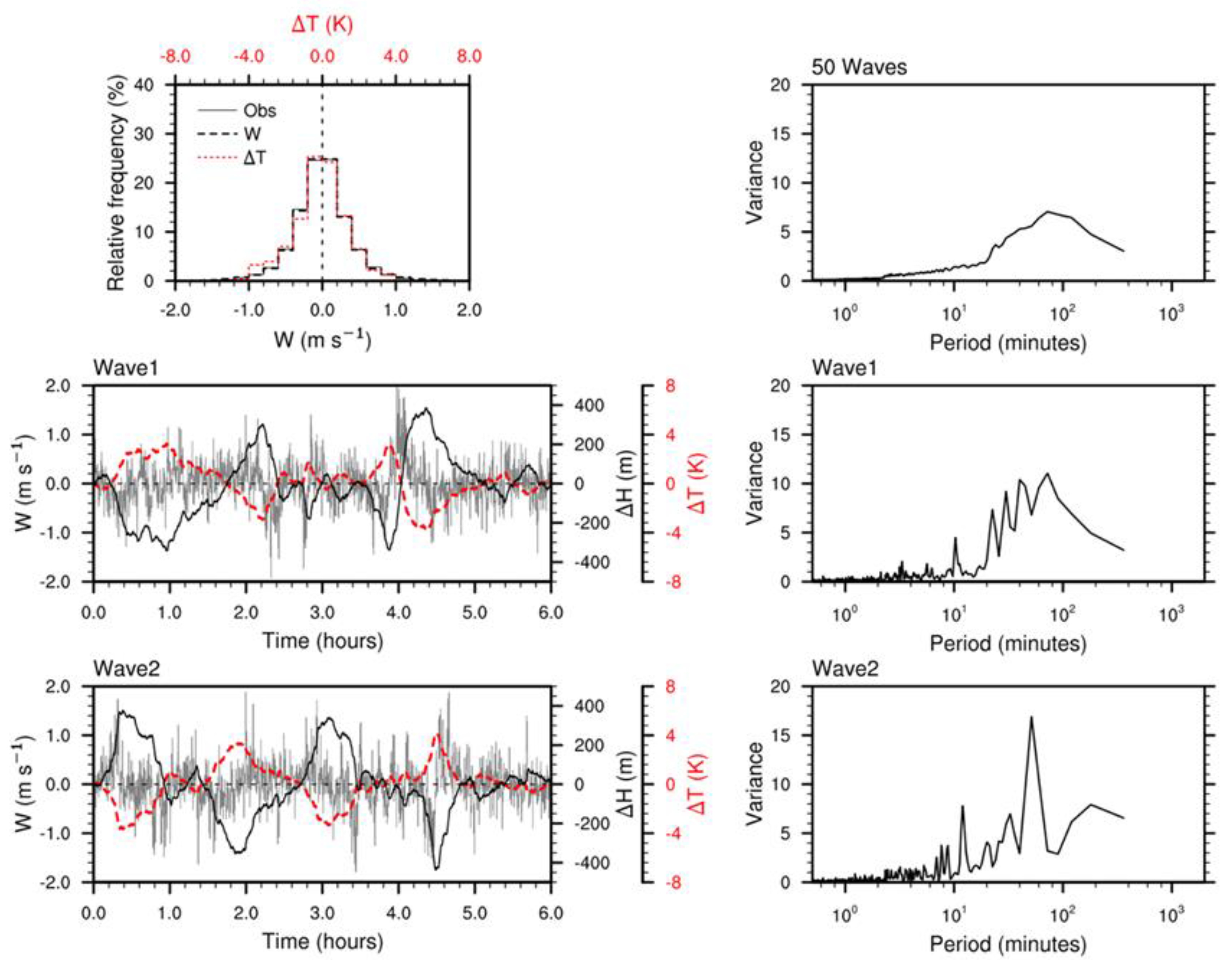
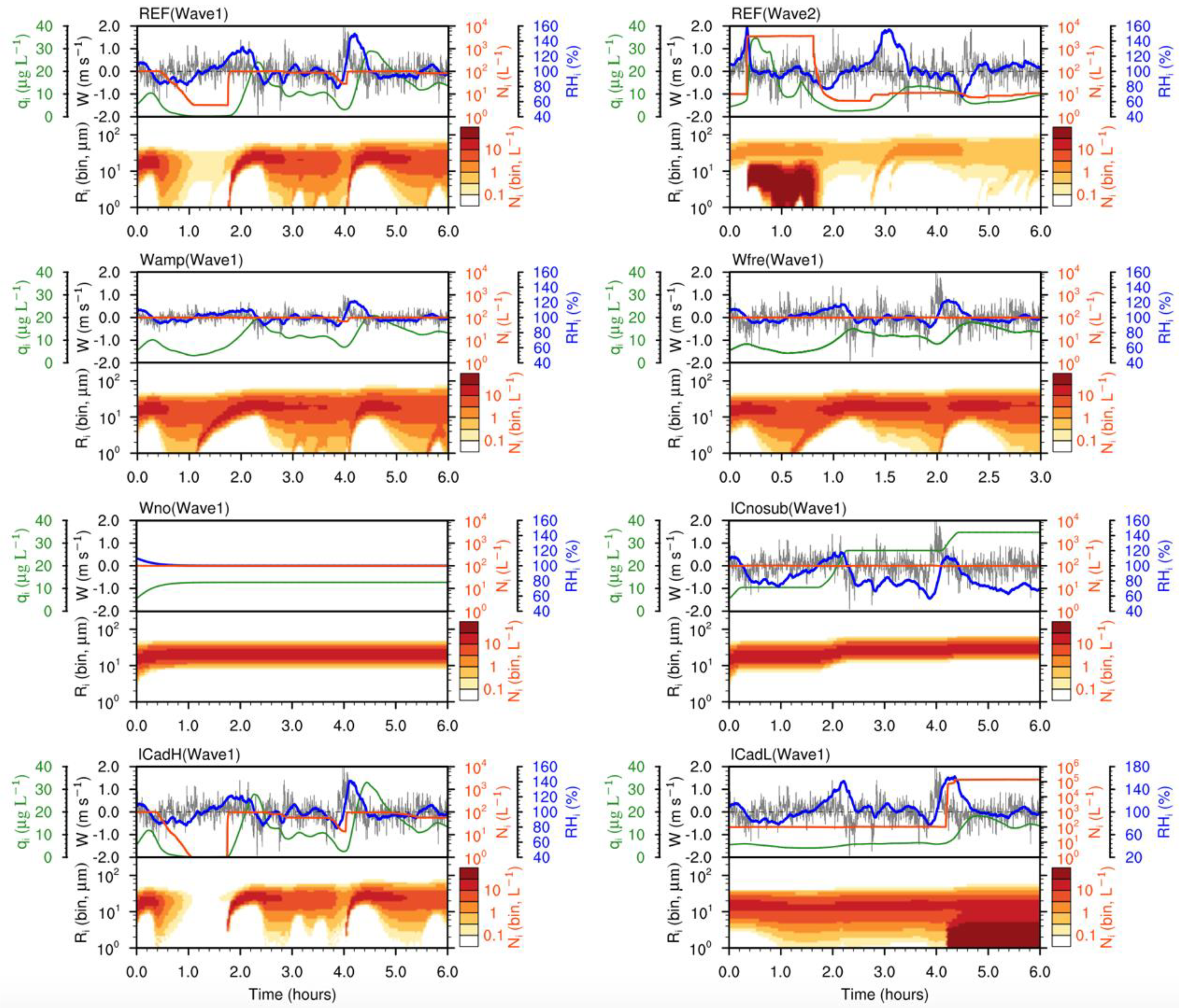
3.1. Case Studies
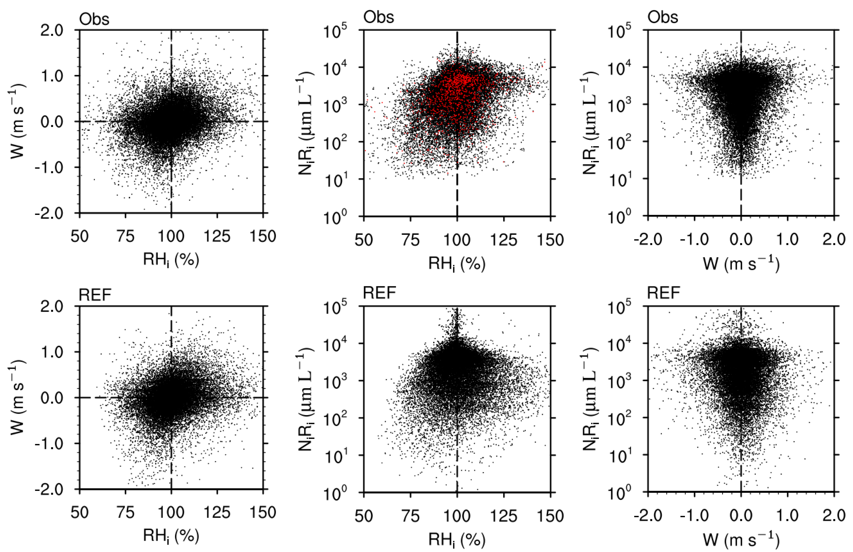
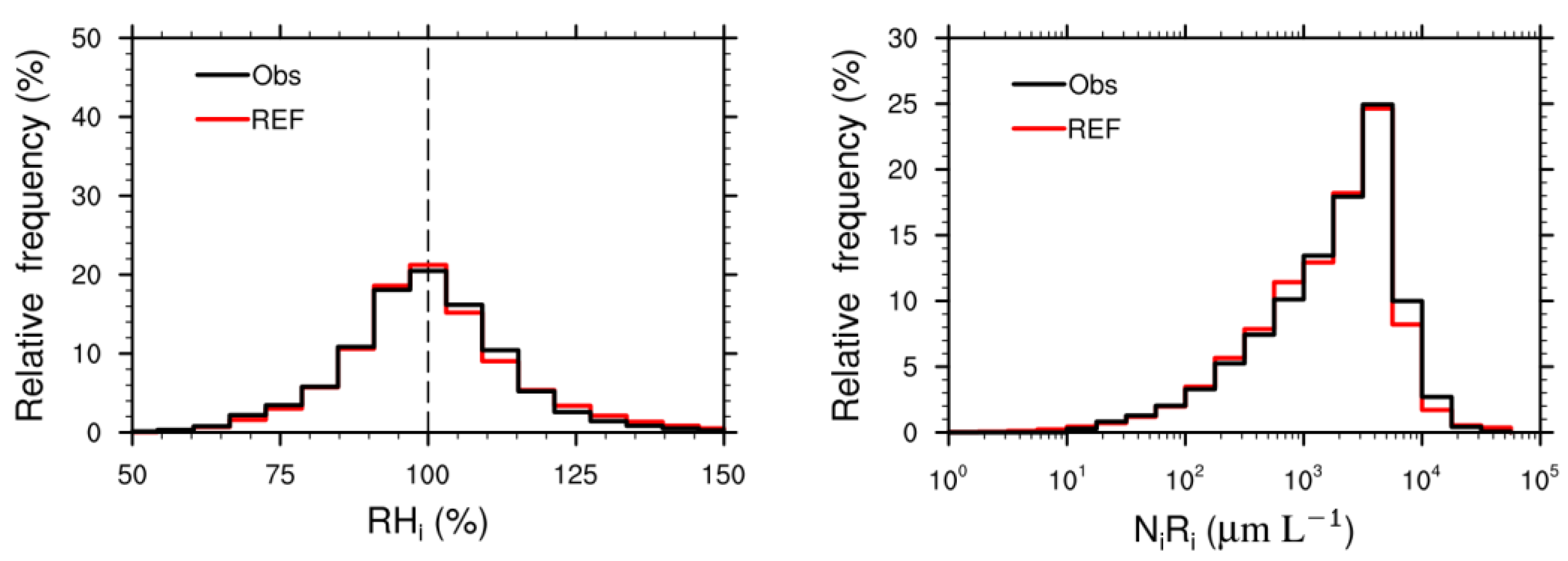
3.2. Comparisons between the REF Experiment and Observations
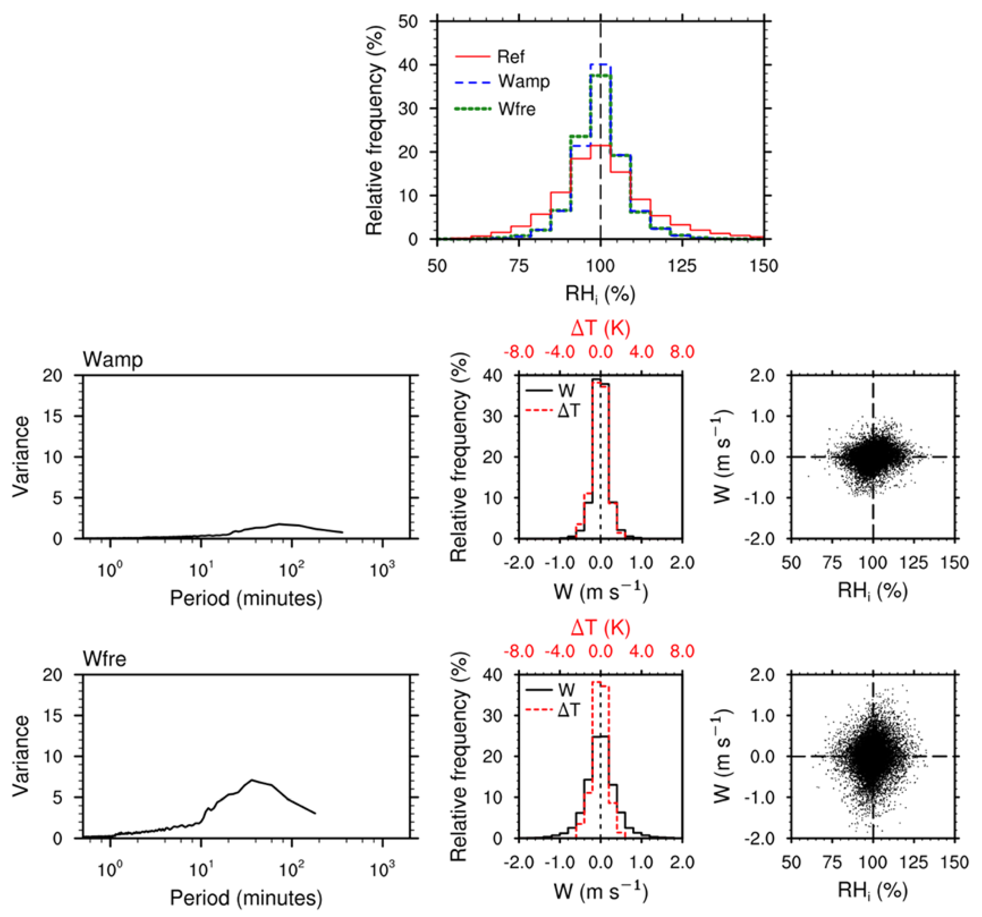
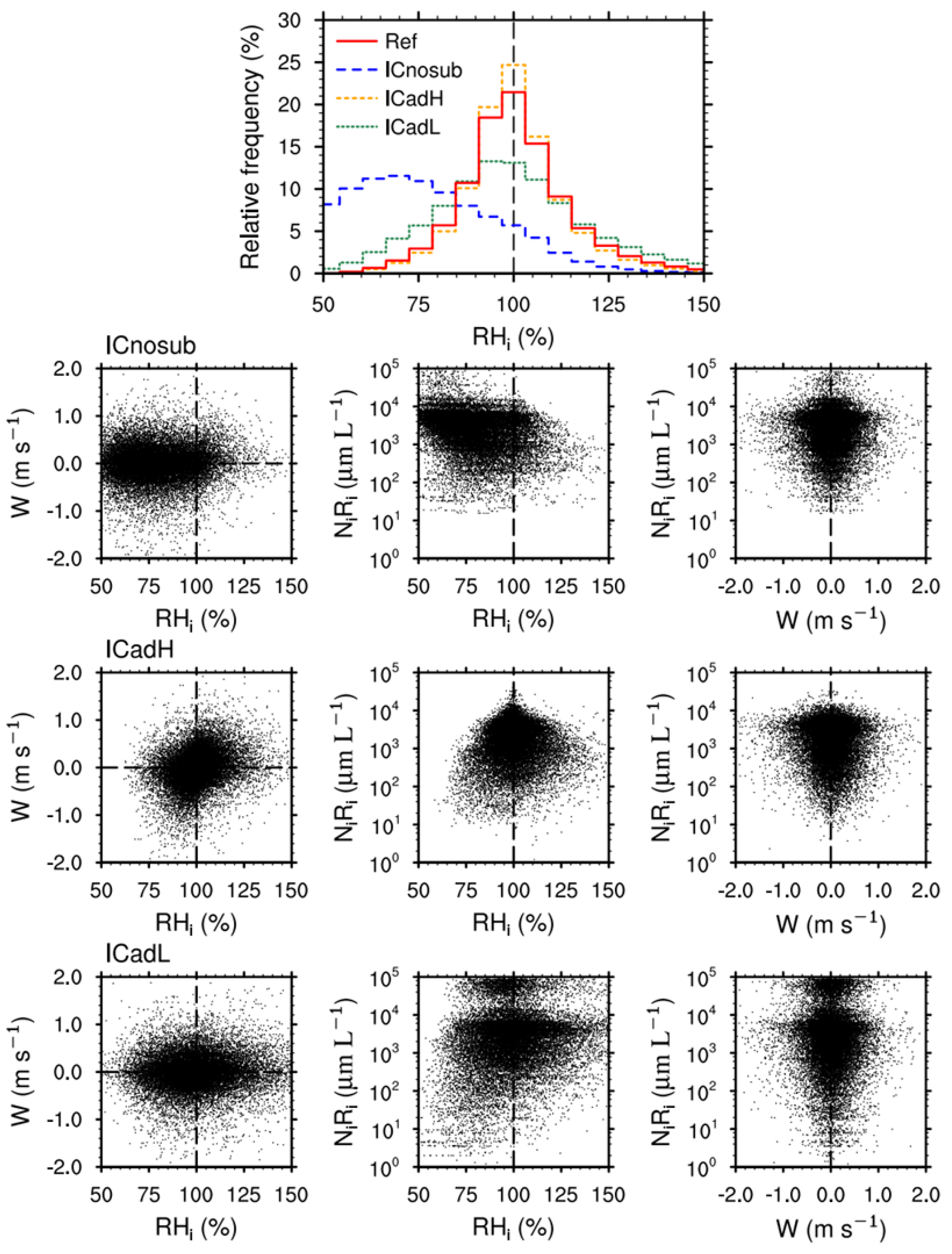
3.3. Deep Analysis through Sensitivity Experiments
4. Discussion
5. Conclusions
Author Contributions
Funding
Institutional Review Board Statement
Informed Consent Statement
Data Availability Statement
Acknowledgments
Conflicts of Interest
References
- Liou, K.-N. Influence of Cirrus Clouds on Weather and Climate Processes: A Global Perspective. Mon. Weather Rev. 1986, 114, 1167–1199. [Google Scholar] [CrossRef]
- Wang, P.-H.; Minnis, P.; McCormick, M.P.; Kent, G.S.; Skeens, K.M. A 6-year climatology of cloud occurrence frequency from Stratospheric Aerosol and Gas Experiment II observations (1985-1990). J. Geophys. Res. Atmos. 1996, 101, 29407–29429. [Google Scholar] [CrossRef]
- Luo, Z.; Rossow, W.B. Characterizing Tropical Cirrus Life Cycle, Evolution, and Interaction with Upper-Tropospheric Water Vapor Using Lagrangian Trajectory Analysis of Satellite Observations. J. Clim. 2004, 17, 4541–4563. [Google Scholar] [CrossRef]
- Gayet, J.-F.; Shcherbakov, V.; Mannstein, H.; Minikin, A.; Schumann, U.; Ström, J.; Petzold, A.; Ovarlez, J.; Immler, F. Microphysical and optical properties of midlatitude cirrus clouds observed in the southern hemisphere during INCA. Q. J. R. Meteorol. Soc. 2006, 132, 2719–2748. [Google Scholar] [CrossRef]
- Korolev, A.; Isaac, G.A. Relative Humidity in Liquid, Mixed-Phase, and Ice Clouds. J. Atmos. Sci. 2006, 63, 2865–2880. [Google Scholar] [CrossRef] [Green Version]
- Sassen, K.; Wang, Z.; Liu, D. Global distribution of cirrus clouds from CloudSat/Cloud-Aerosol Lidar and Infrared Pathfinder Satellite Observations (CALIPSO) measurements. J. Geophys. Res. Atmos. 2008, 113, D00A12. [Google Scholar] [CrossRef]
- Bony, S.; Stevens, B.; Frierson, D.M.W.; Jakob, C.; Kageyama, M.; Pincus, R.; Shepherd, T.G.; Sherwood, S.C.; Siebesma, A.P.; Sobel, A.H.; et al. Clouds, circulation and climate sensitivity. Nat. Geosci. 2015, 8, 261–268. [Google Scholar] [CrossRef] [Green Version]
- Zhou, C.; Penner, J.E.; Lin, G.; Liu, X.; Wang, M. What controls the low ice number concentration in the upper troposphere. Atmos. Meas. Tech. 2016, 16, 12411–12424. [Google Scholar] [CrossRef] [Green Version]
- Barahona, D.; Molod, A.; Kalesse, H. Direct estimation of the global distribution of vertical velocity within cirrus clouds. Sci. Rep. 2017, 7, 6840. [Google Scholar] [CrossRef] [PubMed] [Green Version]
- Ovarlez, J.; Gayet, J.-F.; Gierens, K.; Ström, J.; Ovarlez, H.; Auriol, F.; Busen, R.; Schumann, U. Water vapour measurements inside cirrus clouds in Northern and Southern hemispheres during INCA. Geophys. Res. Lett. 2002, 29, 60–61. [Google Scholar] [CrossRef] [Green Version]
- Comstock, J.M.; Ackerman, T.P.; Turner, D.D. Evidence of high ice supersaturation in cirrus clouds using ARM Raman lidar measurements. Geophys. Res. Lett. 2004, 31, 293–317. [Google Scholar] [CrossRef] [Green Version]
- Krämer, M.; Schiller, C.; Afchine, A.; Bauer, R.; Gensch, I.; Mangold, A.; Schlicht, S.; Spelten, N.; Sitnikov, N.; Borrmann, S.; et al. Ice supersaturations and cirrus cloud crystal numbers. Atmos. Meas. Tech. 2009, 9, 3505–3522. [Google Scholar] [CrossRef] [Green Version]
- Jensen, E.J.; Lawson, R.P.; Bergman, J.W.; Pfister, L.; Bui, T.P.; Schmitt, C.G. Physical processes controlling ice concentrations in synoptically forced, midlatitude cirrus. J. Geophys. Res. Atmos. 2013, 118, 5348–5360. [Google Scholar] [CrossRef]
- Cziczo, D.J.; Froyd, K.D.; Hoose, C.; Jensen, E.J.; Diao, M.; Zondlo, M.A.; Smith, J.B.; Twohy, C.H.; Murphy, D.M. Clarifying the Dominant Sources and Mechanisms of Cirrus Cloud Formation. Science 2013, 340, 1320–1324. [Google Scholar] [CrossRef] [PubMed] [Green Version]
- Spichtinger, P.; Gierens, K.M. Modelling of cirrus clouds—Part 1a: Model description and validation. Atmos. Meas. Tech. 2009, 9, 685–706. [Google Scholar] [CrossRef] [Green Version]
- Kärcher, B. Supersaturation Fluctuations in Cirrus Clouds Driven by Colored Noise. J. Atmos. Sci. 2012, 69, 435–443. [Google Scholar] [CrossRef] [Green Version]
- Krämer, M.; Rolf, C.; Spelten, N.; Afchine, A.; Fahey, D.; Jensen, E.; Khaykin, S.; Kuhn, T.; Lawson, P.; Lykov, A.; et al. A microphysics guide to cirrus—Part 2: Climatologies of clouds and humidity from observations. Atmos. Meas. Tech. 2020, 20, 12569–12608. [Google Scholar] [CrossRef]
- Diao, M.; Zondlo, M.A.; Heymsfield, A.J.; Avallone, L.M.; Paige, M.E.; Beaton, S.P.; Campos, T.; Rogers, D.C. Cloud-scale ice-supersaturated regions spatially correlate with high water vapor heterogeneities. Atmos. Meas. Tech. 2014, 14, 2639–2656. [Google Scholar] [CrossRef] [Green Version]
- Murphy, D.M. Rare temperature histories and cirrus ice number density in a parcel and a one-dimensional model. Atmos. Meas. Tech. 2014, 14, 13013–13022. [Google Scholar] [CrossRef] [Green Version]
- Muhlbauer, A.; Berry, E.; Comstock, J.M.; Mace, G.G. Perturbed physics ensemble simulations of cirrus on the cloud system-resolving scale. J. Geophys. Res. Atmos. 2014, 119, 4709–4735. [Google Scholar] [CrossRef]
- Dinh, T.; Podglajen, A.; Hertzog, A.; Legras, B.; Plougonven, R. Effect of gravity wave temperature fluctuations on homogeneous ice nucleation in the tropical tropopause layer. Atmos. Meas. Tech. 2016, 16, 35–46. [Google Scholar] [CrossRef] [Green Version]
- Podglajen, A.; Plougonven, R.; Hertzog, A.; Jensen, E. Impact of gravity waves on the motion and distribution of atmospheric ice particles. Atmos. Meas. Tech. 2018, 18, 10799–10823. [Google Scholar] [CrossRef] [Green Version]
- Horner, G.A.; Gryspeerdt, E. The evolution of deep convective systems and their associated cirrus outflows. Atmos. Chem. Phys. Discuss. 2022, 1–22. [Google Scholar] [CrossRef]
- Maciel, F.V.; Diao, M.; Patnaude, R. Examination of aerosol indirect effects during cirrus cloud evolution. Atmos. Meas. Tech. 2023, 23, 1103–1129. [Google Scholar] [CrossRef]
- Stommel, H. Entrainment of Air into a Cumulus Cloud. J. Meteorol. 1947, 4, 91–94. [Google Scholar] [CrossRef]
- Burnet, F.; Brenguier, J.-L. Observational Study of the Entrainment-Mixing Process in Warm Convective Clouds. J. Atmos. Sci. 2007, 64, 1995–2011. [Google Scholar] [CrossRef]
- Pinsky, M.; Khain, A. Theoretical Analysis of the Entrainment–Mixing Process at Cloud Boundaries. Part II: Motion of Cloud Interface. J. Atmos. Sci. 2019, 76, 2599–2616. [Google Scholar] [CrossRef]
- Lu, C.; Liu, Y.; Niu, S. Examination of turbulent entrainment-mixing mechanisms using a combined approach. J. Geophys. Res. Atmos. 2011, 116, D20. [Google Scholar] [CrossRef]
- Yum, S.S.; Wang, J.; Liu, Y.; Senum, G.; Springston, S.; McGraw, R.; Yeom, J.M. Cloud microphysical relationships and their implication on entrainment and mixing mechanism for the stratocumulus clouds measured during the VOCALS project. J. Geophys. Res. Atmos. 2015, 120, 5047–5069. [Google Scholar] [CrossRef]
- Ghate, V.P.; Cadeddu, M.P. Drizzle and Turbulence Below Closed Cellular Marine Stratocumulus Clouds. J. Geophys. Res. Atmos. 2019, 124, 5724–5737. [Google Scholar] [CrossRef] [Green Version]
- Desai, N.; Liu, Y.; Glienke, S.; Shaw, R.A.; Lu, C.; Wang, J.; Gao, S. Vertical Variation of Turbulent Entrainment Mixing Processes in Marine Stratocumulus Clouds Using High-Resolution Digital Holography. J. Geophys. Res. Atmos. 2021, 126, e2020JD033527. [Google Scholar] [CrossRef]
- Pruppacher, H.; Klett, J. Microphysics of Clouds and Precipitation, 2nd ed.; Kluwer Academic Publishers: New York, NY, USA, 1996; pp. 502–561. [Google Scholar] [CrossRef]
- Haag, W. The impact of aerosols and gravity waves on cirrus clouds at midlatitudes. J. Geophys. Res. Atmos. 2004, 109, D12. [Google Scholar] [CrossRef] [Green Version]
- Jensen, E.; Pfister, L.; Bui, T.; Weinheimer, A.; Weinstock, E.; Smith, J.; Pittman, J.; Baumgardner, D.; Lawson, P.; McGill, M.J. Formation of a tropopause cirrus layer observed over Florida during CRYSTAL-FACE. J. Geophys. Res. Atmos. 2005, 110, D3. [Google Scholar] [CrossRef] [Green Version]
- Schiller, C.; Krämer, M.; Afchine, A.; Spelten, N.; Sitnikov, N. Ice water content of Arctic, midlatitude, and tropical cirrus. J. Geophys. Res. Atmos. 2008, 113, D24. [Google Scholar] [CrossRef] [Green Version]
- Kärcher, B.; Burkhardt, U. A cirrus cloud scheme for general circulation models. Q. J. R. Meteorol. Soc. 2008, 134, 1439–1461. [Google Scholar] [CrossRef] [Green Version]
- Barahona, D.; Nenes, A. Dynamical states of low temperature cirrus. Atmos. Meas. Tech. 2011, 11, 3757–3771. [Google Scholar] [CrossRef] [Green Version]
- Shi, X.; Liu, X. Effect of cloud-scale vertical velocity on the contribution of homogeneous nucleation to cirrus formation and radiative forcing. Geophys. Res. Lett. 2016, 43, 6588–6595. [Google Scholar] [CrossRef] [Green Version]
- Krämer, M.; Rolf, C.; Luebke, A.; Afchine, A.; Spelten, N.; Costa, A.; Meyer, J.; Zöger, M.; Smith, J.; Herman, R.L.; et al. A microphysics guide to cirrus clouds—Part 1: Cirrus types. Atmos. Meas. Tech. 2016, 16, 3463–3483. [Google Scholar] [CrossRef] [Green Version]
- Jensen, E.J.; Diskin, G.S.; DiGangi, J.; Woods, S.; Lawson, R.P.; Bui, T.V. Homogeneous Freezing Events Sampled in the Tropical Tropopause Layer. J. Geophys. Res. Atmos. 2022, 127, e2022JD036535. [Google Scholar] [CrossRef]
- Strandgren, J. The Life Cycle of Anvil Cirrus Clouds from a Combination of Passive and Active Satellite Remote Sensing. Ph.D. Thesis, The Ludwig Maximilian University, München, Germany, 6 September 2018. [Google Scholar] [CrossRef]
- Rollins, A.W.; Thornberry, T.D.; Gao, R.S.; Smith, J.B.; Sayres, D.S.; Sargent, M.R.; Schiller, C.; Krämer, M.; Spelten, N.; Hurst, D.F.; et al. Evaluation of UT/LS hygrometer accuracy by intercomparison during the NASA MACPEX mission. J. Geophys. Res. Atmos. 2014, 119, 1915–1935. [Google Scholar] [CrossRef] [PubMed]
- Xu, Z.; Mace, G.G. Ice Particle Mass–Dimensional Relationship Retrieval and Uncertainty Evaluation Using the Optimal Estimation Methodology Applied to the MACPEX Data. J. Appl. Meteorol. Clim. 2017, 56, 767–788. [Google Scholar] [CrossRef]
- Scott, S.G.; Bui, T.P.; Chan, K.R.; Bowen, S.W. The Meteorological Measurement System on the NASA ER-2 Aircraft. J. Atmos. Ocean. Technol. 1990, 7, 525–540. [Google Scholar] [CrossRef]
- Weinstock, E.M.; Hintsa, E.J.; Dessler, A.E.; Oliver, J.F.; Hazen, N.L.; Demusz, J.N.; Allen, N.T.; Lapson, L.B.; Anderson, J.G. New fast response photofragment fluorescence hygrometer for use on the NASA ER-2 and the Perseus remotely piloted aircraft. Rev. Sci. Instrum. 1994, 65, 3544–3554. [Google Scholar] [CrossRef]
- Murphy, D.M.; Koop, T. Review of the vapour pressures of ice and supercooled water for atmospheric applications. Q. J. R. Meteorol. Soc. 2005, 131, 1539–1565. [Google Scholar] [CrossRef]
- Lawson, R.P.; O’Connor, D.; Zmarzly, P.; Weaver, K.; Baker, B.; Mo, Q.; Jonsson, H. The 2D-S (Stereo) Probe: Design and Preliminary Tests of a New Airborne, High-Speed, High-Resolution Particle Imaging Probe. J. Atmos. Ocean. Technol. 2006, 23, 1462–1477. [Google Scholar] [CrossRef] [Green Version]
- Khvorostyanov, V.I.; Sassen, K. Microphysical processes in cirrus and their impact on radiation: A mesoscale modeling perspective. In Cirrus, 1st ed.; Lynch, D.K., Sassen, K., Starr, D.O.C., Stephens, G., Eds.; Oxford University Press: New York, NY, USA, 2002; Chapter 19; pp. 397–432. [Google Scholar] [CrossRef]
- Wang, M.; Liu, X.; Zhang, K.; Comstock, J.M. Aerosol effects on cirrus through ice nucleation in the Community Atmosphere Model CAM5 with a statistical cirrus scheme. J. Adv. Model. Earth Syst. 2014, 6, 756–776. [Google Scholar] [CrossRef]
- Kärcher, B.; Podglajen, A. A Stochastic Representation of Temperature Fluctuations Induced by Mesoscale Gravity Waves. J. Geophys. Res. Atmos. 2019, 124, 11506–11529. [Google Scholar] [CrossRef] [Green Version]
- Lu, X.; Chu, X.; Li, H.; Chen, C.; Smith, J.A.; Vadas, S.L. Statistical characterization of high-to-medium frequency mesoscale gravity waves by lidar-measured vertical winds and temperatures in the MLT. J. Atmos. Sol. -Terr. Phys. 2017, 162, 3–15. [Google Scholar] [CrossRef]
- Kalesse, H.; Kollias, P. Climatology of High Cloud Dynamics Using Profiling ARM Doppler Radar Observations. J. Clim. 2013, 26, 6340–6359. [Google Scholar] [CrossRef]
- Gierens, K.M.; Monier, M.; Gayet, J. The deposition coefficient and its role for cirrus clouds. J. Geophys. Res. Atmos. 2003, 108, D2. [Google Scholar] [CrossRef]
- Skrotzki, J.; Connolly, P.; Schnaiter, M.; Saathoff, H.; Möhler, O.; Wagner, R.; Niemand, M.; Ebert, V.; Leisner, T. The accommodation coefficient of water molecules on ice-cirrus cloud studies at the AIDA simulation chamber. Atmos. Meas. Tech. 2013, 13, 4451–4466. [Google Scholar] [CrossRef] [Green Version]
- Korolev, A.V.; Mazin, I.P. Supersaturation of Water Vapor in Clouds. J. Atmos. Sci. 2003, 60, 2957–2974. [Google Scholar] [CrossRef]
- Zhang, W.; Shi, X.; Lu, C. Impacts of the ice-particle size distribution shape parameter on climate simulations with the Community Atmosphere Model Version 6 (CAM6). Geosci. Model Dev. 2022, 15, 7751–7766. [Google Scholar] [CrossRef]
- Jensen, E.J.; Ueyama, R.; Pfister, L.; Bui, T.V.; Alexander, M.J.; Podglajen, A.; Hertzog, A.; Woods, S.; Lawson, R.P.; Kim, J.; et al. High-frequency gravity waves and homogeneous ice nucleation in tropical tropopause layer cirrus. Geophys. Res. Lett. 2016, 43, 6629–6635. [Google Scholar] [CrossRef]
- Mascio, J.; Mace, G.G. Quantifying uncertainties in radar forward models through a comparison between CloudSat and SPartICus reflectivity factors. J. Geophys. Res. Atmos. 2017, 122, 1665–1684. [Google Scholar] [CrossRef]


| Experiment | Description |
|---|---|
| REF | Reference experiment. The αd is 0.05. |
| Sensitivity experiments for vertical motion | |
| Wamp | Same as REF, but the amplitude of the W time series is reduced to half. |
| Wfre | Same as REF, but the frequency of the W time series is doubled. |
| Wno | Same as REF, but W has a constant value of 0. |
| Sensitivity experiments for the IC deposition/sublimation process. | |
| ICnosub | Same as REF, but the sublimation process is not allowed. |
| ICadH | Same as REF, but the αd is set to 1.0. |
| ICadL | Same as REF, but the αd is set to 0.001. |
Disclaimer/Publisher’s Note: The statements, opinions and data contained in all publications are solely those of the individual author(s) and contributor(s) and not of MDPI and/or the editor(s). MDPI and/or the editor(s) disclaim responsibility for any injury to people or property resulting from any ideas, methods, instructions or products referred to in the content. |
© 2023 by the authors. Licensee MDPI, Basel, Switzerland. This article is an open access article distributed under the terms and conditions of the Creative Commons Attribution (CC BY) license (https://creativecommons.org/licenses/by/4.0/).
Share and Cite
Zhao, M.; Shi, X. A Study on the Wide Range of Relative Humidity in Cirrus Clouds Using Large-Ensemble Parcel Model Simulations. Atmosphere 2023, 14, 583. https://doi.org/10.3390/atmos14030583
Zhao M, Shi X. A Study on the Wide Range of Relative Humidity in Cirrus Clouds Using Large-Ensemble Parcel Model Simulations. Atmosphere. 2023; 14(3):583. https://doi.org/10.3390/atmos14030583
Chicago/Turabian StyleZhao, Miao, and Xiangjun Shi. 2023. "A Study on the Wide Range of Relative Humidity in Cirrus Clouds Using Large-Ensemble Parcel Model Simulations" Atmosphere 14, no. 3: 583. https://doi.org/10.3390/atmos14030583