Article

Thermospheric NO Cooling during an Unusual Geomagnetic Storm of 21–22 January 2005: A Comparative Study between TIMED/SABER Measurements and TIEGCM Simulations

1
National Institute of Polar Research, Tokyo 190-8518, Japan
2
GFZ German Centre for Geosciences, 14473 Potsdam, Germany
3
Department of Physics, Indian Institute of Technology Roorkee, Roorkee 247667, India
*
Authors to whom correspondence should be addressed.
Atmosphere 2023, 14(3), 556; https://doi.org/10.3390/atmos14030556
Submission received: 9 February 2023 / Revised: 9 March 2023 / Accepted: 10 March 2023 / Published: 14 March 2023
(This article belongs to the Special Issue Structure and Dynamics of Mesosphere and Lower Thermosphere)

Abstract

:
The geomagnetic storm is the manifestation of the solar wind–magnetosphere interaction. It deposits huge amount of the solar energy into the magnetosphere–ionosphere–thermosphere (MIT) system. This energy creates global perturbations in the chemistry, dynamics, and energetics of the MIT system. The high latitude energy deposition results in the Joule and particle heating that subsequently increases the thermospheric temperature. The thermospheric temperature is effectively regulated by the process of thermospheric cooling emission by nitric oxide via 5.3 µm. A peculiar, intense geomagnetic storm (Dst = −105 nT) occurred during 21–22 January 2005, where the main phase developed during the northward orientation of the z-component of interplanetary magnetic field. We utilized the nitric oxide 5.3 µm infrared emission from the NCAR’s Thermosphere–Ionosphere–Electrodynamics General Circulation Model (TIEGCM) simulation and the Sounding of Atmosphere using Broadband Emission Radiometry (SABER) onboard the thermosphere–ionosphere–mesosphere energetic and dynamics satellite to investigate its response to this anomalous geomagnetic storm. We compared the model results with the observations on both the local and global scales. It is observed that the model results agree very well with the observations during quiet times. However, the model severely underestimates the cooling emission by one-fourth of the observations, although it predicts an enhancement in the thermospheric temperature and densities of atomic oxygen and nitric oxide during the geomagnetic storm.

1. Introduction

The solar wind embedded in the southward interplanetary magnetic field (IMF) results in the formation of geomagnetic storm when it interacts with the Earth’s dayside magnetosphere. The directional orientation of the interplanetary magnetic field plays an important role in transferring the solar wind energy and momentum into the magnetosphere. The solar wind coupling efficiency during northward IMF is approximately two orders of magnitude lower than that during southward IMF [1]. The southward IMF transfers enormous energy due to a strong reconnection process [2,3]. This process of geomagnetic storm deposits huge amount of energy and momentum into the Earth’s high latitude region. It can modulate the chemistry, structure, energetics, and dynamics all over the globe. However, although it is not usual, the northward IMF can sometimes create a geomagnetic storm [3]. One of such events occurred during 21–22 January 2005, where the growth of the Dst index was observed under the northward IMF Bz condition [3,4]. Although it was a moderate geomagnetic storm with a number of anomalous features, some of its features behaved like a typical superstorm. It was driven by one of the fastest interplanetary coronal mass ejections (ICME) of the 23rd solar cycle [4]. This geomagnetic storm created some of the unexpected phenomena in the Earth’s atmosphere that are generally observed during superstorms [4]. This geomagnetic storm also created some of the unusual phenomena in the Earth’s equatorial ionosphere. For example, there was immediate lifting of the equatorial F2 region at the first impacts of shock. Similarly, the F3 layer rose to approximately 1200 km altitude. Sahai et al. (2011) [5], by using total electron content (TEC), also reported an unusual intensification of the equatorial ionization anomaly (EIA).
The condition of the interplanetary medium that led to the anomalous storm of 21–22 January 2005, was extensively studied by Manchester et al. (2014) [6] by using a three-dimensional magnetohydrodynamic model. The simulation predicted the magnetic reconnection between the northward IMF in the sheath and the southward IMF in the CME. This simulation was also supported by the cluster satellite observation in the solar wind upstream of the Earth. The dense plasma travelling behind the ICME sheath region, which was observed during the Carrington event of 1859 [7] and 4–5 August 1972 solar event [8], was instrumental in developing a superstorm-like geomagnetic storm and damaging the geospace instruments. The high-speed solar wind, strong IMF By, and the solar wind pressure elevated the Joule heating in the polar cusp to that observed during superstorms. In the present investigation, the response of the NO cooling flux is studied during this unusual event by using both observations and modeling.
The nitric oxide radiative emission at 5.3 µm is the dominating radiative coolant in the thermosphere in the altitude region of 100–300 km [9,10]. It results primarily due to the inelastic collision of nitric oxide with atomic oxygen density.
NO ν = 1 + O NO ν = 0 + O  
In low latitude sun-lit condition, the interaction of the atomic nitrogen (N2D) with molecular oxygen produces NO [11,12,13]. In addition, the particle precipitation creates nitric oxide via a series of chemical reactions, e.g., auroral electrons of energy 1–10 keV and ions with energy of 10–20 keV dissociate N2 to produce N(2D) in the altitude range of 100–200 km. Further, the dissociation of N2 by auroral electron with 0.3–0.9 keV energy range produces N(4S) [11,12,13]. These nitrogen atoms interact with molecular oxygen to create NO as follows:
N ( 4 S , 2 D ) + O 2 NO + O
This reaction mechanism is important above 110 km due to the fact that it is highly sensitive to the temperature.
In the present study, we investigated the TIEGCM (Thermosphere Ionosphere Electrodynamics General Circulation Model) model results of nitric oxide 5.3 µm infrared emission along with the TIMED-SABER satellite observations during the 21–22 January 2005, event (TIMED-Thermosphere Ionosphere Mesosphere Energetics Dynamics; SABER-Sounding of Atmosphere using Broadband Emission Radiometry). We divide this paper into five sections. Section 2 provides a brief introduction of the data sets and analysis method used in this study. It also includes the various geomagnetic indices and interplanetary solar wind parameters used. The corresponding response of the thermospheric nitric oxide emission and possible causes are discussed in the Section 3 and Section 4 using the model and satellite observations. We conclude this paper with a summary in Section 5.

2. Data Acquisition and Analysis

2.1. Nitric Oxide Radiative Emission

The nitric oxide (NO) emission is one of the dominating coolants in the thermosphere above 100 km. It can effectively convert the kinetic energy into the radiative energy that exits in the thermosphere [10]. In the present study, we utilized the TIMED-SABER satellite observations and the TIEGCM simulations results to investigate the thermospheric nitric oxide cooling during northward interplanetary magnetic field.

2.1.1. TIMED-SABER Satellite Observations

SABER is multichannel limb sounder that covers the hemispheres asymmetrically, from 53° in one hemisphere to 83° in another, during any 60–65-day period due to anti-sunward view. It has an orbital period of approximately 90 min. SABER continuously scans the Earth’s atmosphere to measures infrared radiance in ten channels [14,15]. SABER observes from approximately 400 km down to the surface and back, with a vertical resolution of approximately 0.4 km. The observations include radiative cooling by nitric oxide at 5.3 µm and CO2 at 15 µm, apart from other atmospheric species and heating agents. The NO volume emission rate (Wm−3) is calculated by using an Abel inversion technique to the SABER measured irradiance [10,16,17,18,19]. The volume emission rate is integrated vertically in the altitude of 100 to 250 km to obtain cooling flux (Wm−2). The cooling flux has been binned into a 10° latitude and 20° longitude grid to investigate the latitude–longitude variation. The NO cooling emission has uncertainty better than 15% [17]. In the present study, we used SABER version 2.0 data. During the event presented here, the SABER was in the northern view mode and covered approximately 83° latitude in the northern hemisphere to approximately 53° latitude in the southern hemisphere. The median local times (LT) were, respectively, 5:13 and 6:40 during 21 January and 22 January 2005. SABER observes two local times corresponding to daily ascending and descending modes.

2.1.2. TIEGCM Simulation

The NCAR (National Centre for Atmospheric Research)’s TIEGCM (Thermosphere–Ionosphere–Electrodynamics General Circulation Model) is a time-dependent three-dimensional model based on first principles [20,21]. The coupled nonlinear, thermodynamic, and hydrodynamic continuity equations for the neutrals, ions, and wind, including the ion energy and momentum, are solved self-consistently. The latest version of TIEGCM (v2.0) uses a horizontal grid of 2.5°, both in geographic latitude and longitude. The vertical grid uses 57 pressure surfaces in vertical resolution of ¼ scale height. It covers the altitude of approximately 97 km to approximately 500 km. The TIEGCM is driven by different external forcing, such as solar and magnetic forcing, tidal amplitudes, and phases from lower atmosphere. The solar forcing is parametrized by F10.7 index. The high-latitude electric fields can be obtained from the Heelis model [22] or the Weimer model [23]. The high-latitude precipitation and convection patterns represent the geomagnetic forcing and are obtained from the Weimer model [23] in the present study. The Weimer model is driven by interplanetary magnetic fields, solar wind density, and solar wind speed. The tidal amplitudes and phases are from the Global Scale Wave Model [24]. The TIEGCM simulation was conducted on the NASA Community Coordinated Modeling Center (CCMC) web interface (https://ccmc.gsfc.nasa.gov/). The model output is archived on CCMC website (Archive: Tikemani_Bag_092022_IT_4).
The TIEGCM uses the formulation of Kockarts (1980) [9] to calculate the thermospheric nitric oxide emission, which is given as
NO   5.3   μ m = k o O + k o 2 O 2 k o O + k o 2 O 2 + A 10 h ν A 10 NO e h ν KT
where ko (=4.2 × 10⁻¹¹ cm3 s−1 [25]) and ko2 (=2.4 × 10⁻¹⁴ cm3 s−1 [26]) are, respectively, the relaxation rates of energy transition from NO(v = 1) to NO(v = o) in collision with atomic and molecular oxygen density, and [O], [O2], and [NO] represent the number densities of O, O2, and NO, respectively. A10 is the Einstein’s coefficient (=13.3 s−1), h is Planck’s constant, v is frequency of NO emission, K is Boltzmann constant, and T is the neutral temperature. The TIEGCM simulated nitric oxide cooling has been investigated by many researchers [27,28,29,30,31,32,33,34]. In the present study, the TIEGCM data are sampled at the TIMED/SABER satellite measurement locations and binned into same latitude–longitude grid as SABER. A comparison between the TIMED-SABER satellite measurement and the TIEGCM simulation results during the super storm event of November 2003 is shown in Figure 1. It is clearly evident that the TIEGCM simulation result overestimates the NO cooling flux during the storm period. Similar storm-time overestimation of TIEGCM simulation during moderate and intense storms has been reported by many researchers [26,28,29,31,32,33,34].

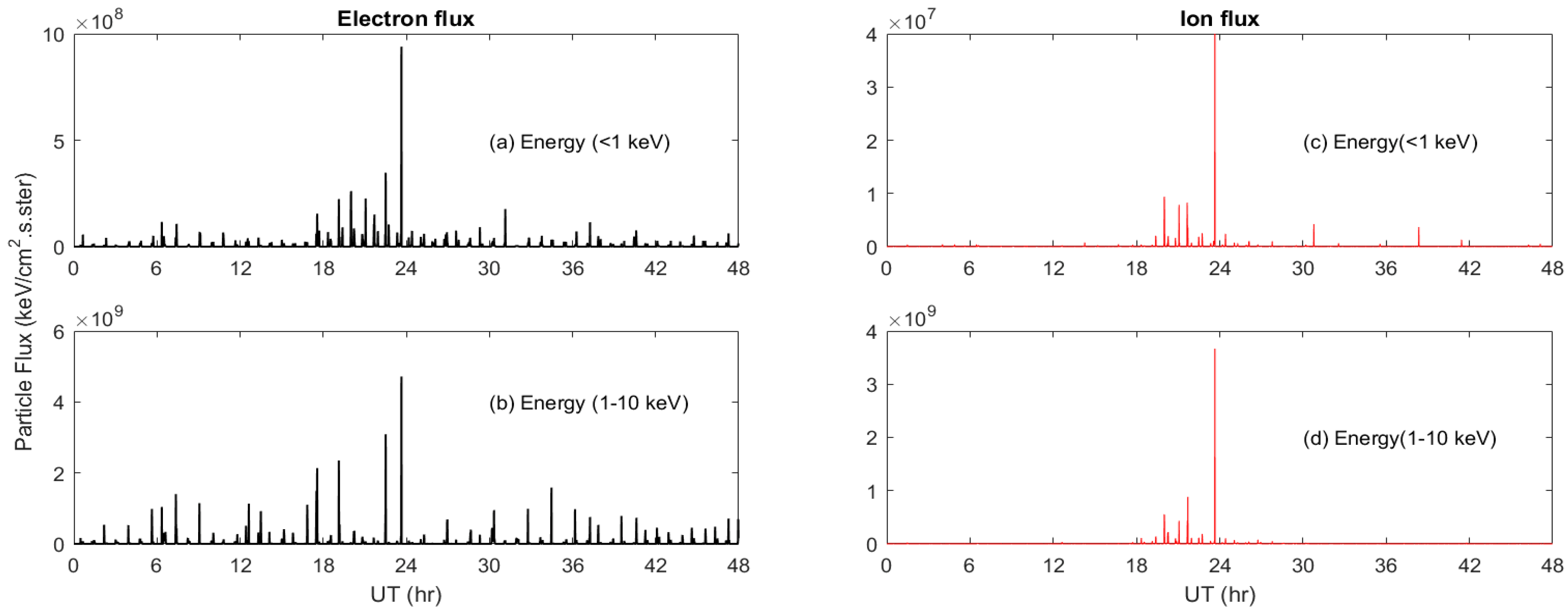
2.2. DMSP Observations of Particle Flux

The production of the high latitude nitric oxide density is strongly affected by particle precipitation. We utilized the Defense Meteorological Satellite Program (DMSP) F15 satellite observations of particle flux to investigate its impacts on the cooling observations. The DMSP is a polar satellite at the circular orbit of approximately 850 km [35]. It has orbital period of approximately 100 min. The DMSP has low energy particle sensor (SSJ/4) onboard to measure auroral particle in 20 energy channels. It covers the energy range of 30 eV to 30 keV every second. The electron and ion data are divided into two ranges in the present study: less than 1 keV and less than 10 keV.

2.3. NOAA Satellite Observation of Hemispheric Power

NOAA (National Oceanic and Atmospheric Administration) is a polar satellite at approximately 870 km. The Total Energy Detector instrument onboard the NOAA satellite measures the energy flux in the range of 0.3 keV to 20 keV at two pitch angles within loss cone. The total power deposited into the northern or southern hemisphere is calculated using the particle flux along the satellite track above 45° magnetic latitude. The particle energy deposited into each high-latitude hemisphere provides the estimation of the hemispheric power [35,36,37].

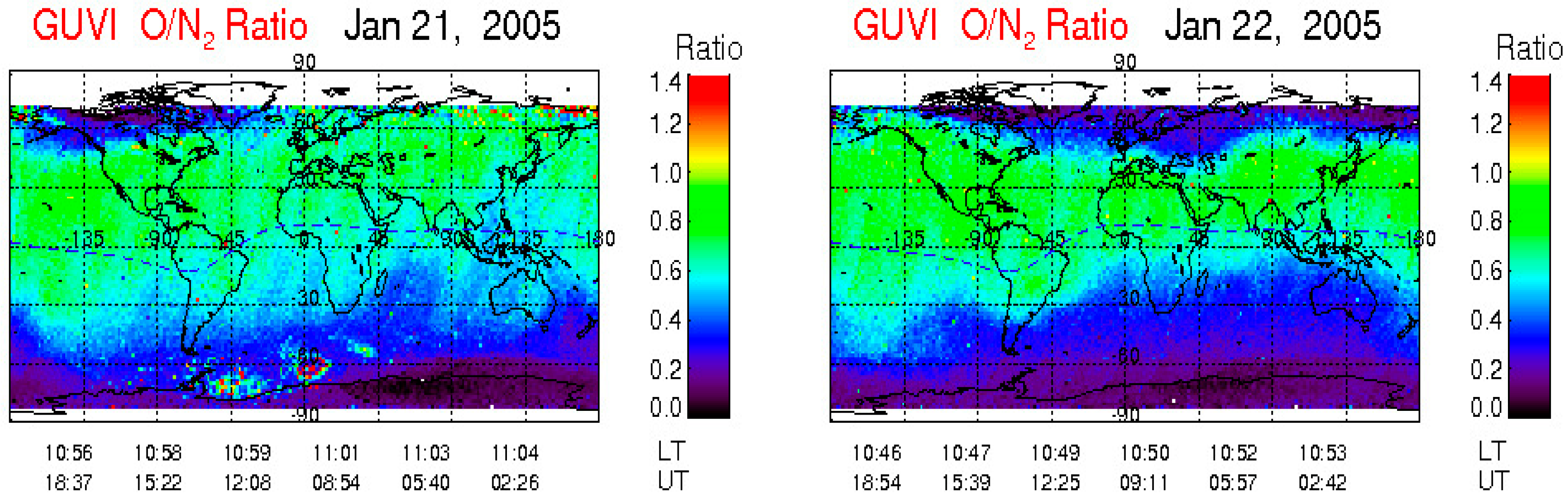
2.4. GUVI Observations of O/N2 Ratio

We utilize the TIMED-GUVI (Global UltraViolet Imager) observations of O/N2 ratio to understand its variation during the event. The GUVI is an ultraviolet imager that measures the far ultraviolet emissions including hydrogen’s Lyman alpha, atomic oxygen lines at 130.4 and 135.6 nm, and N2 LBH bands [38,39]. GUVI scans Earth’s limb and disk and provides far UV airglow emission every 15 seconds, covering a projected area of 2500 km × 100 km at the altitude of 150 km. The O/N2 ratio, derived using atomic oxygen airglow emission at 135.6 nm and LBH band, is referenced to N2 column density of 1017 cm−2. The O/N2 (Level 3), referenced from an altitude of 135 km, is used in the present study [40,41].

3. Results

The CME that erupted on 20 January 2005, from the X7.1/3B solar flare caused a moderate geomagnetic storm on 21 January 2005 [42,43]. Figure 2 shows the solar wind parameters at the L1 point (in geocentric solar magnetospheric coordinate system) as measured by the ACE satellite. These have been shifted by 24 mins to align with the geomagnetic signatures of the first sudden storm commencement (SSC). This storm was characterized mainly by two storm commencements (indicated as SSC-1 and SSC-2 in red dashed lines) associated with two consecutive interplanetary shocks. The ACE satellite detected a large coronal mass ejection (CME) at ∼16:48 UT that arrived at the magnetopause at ∼17:12 UT on 21 January triggering SSC-1, and a few minutes later (at 18:43 UT) another CME shock front arrived that triggered SSC-2. It can be seen that the solar wind parameters (|B|, solar wind density, and velocity) changed sharply at these times. The proton density Np increased from 2 cc−1 to 22 cc−1 during SSC-1 and further increased to an unusually high value of 62 cc−1. The solar wind velocity increased from 565 km/s to 900 km/s. The solar wind dynamic pressure increased from 2 nPa to 35 nPa during the SSC-1, and then it increased to the significantly high value of 106 nPa during SSC-2. In response to SSC-1, the SYM-H increased from −17 nT to 55 nT. A few minutes later (at 18:43 UT), the second shock front arrived, causing the SSC-2 that led to a second increase in the SYM-H value. It is around this time that the IMF Bz turned northward, but surprisingly, the storm’s main phase continued to develop. The SYM-H reached its lowest value of −105 nT at 06:00 UT on 22 January. The IMF Bz was continuously northward from 19:40 UT, 21 January to 02:45 UT, 22 January 2005. Typically, when the IMF Bz turns northward, the ring current starts to recover. But surprisingly, in this case, the ring current grew under the IMF Bz condition for more than 10 h. This apparently “anomalous” behavior was first reported by Du et al. (2008) [3].

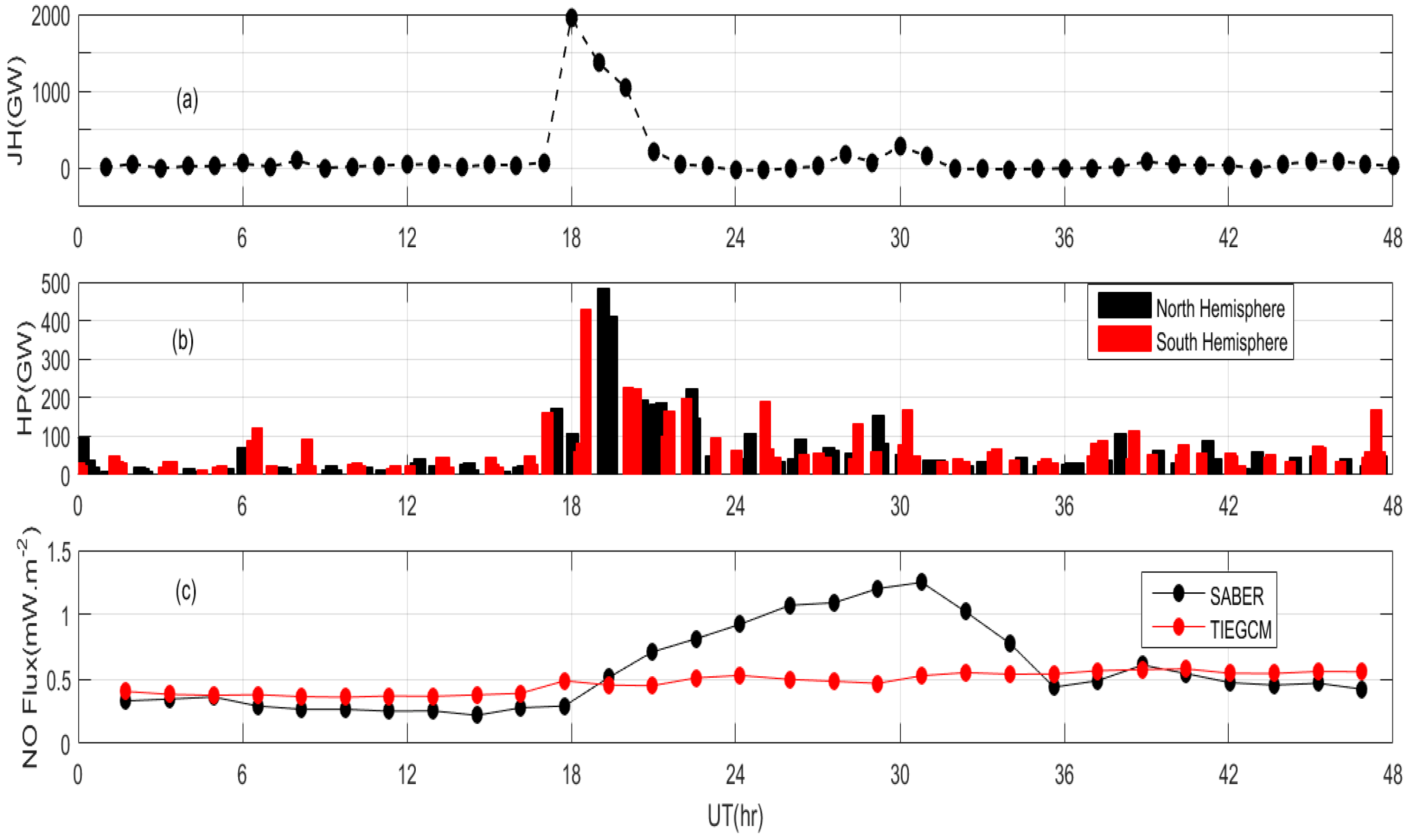
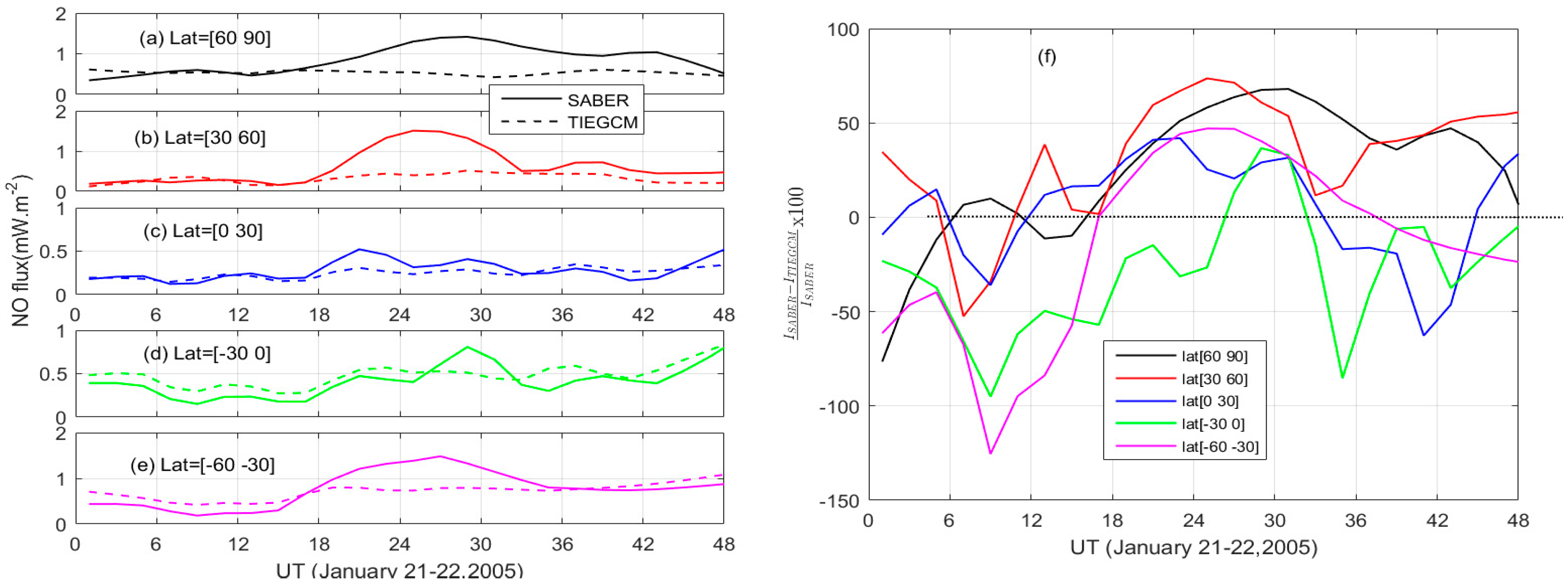
3.1. Orbital Variation of Cooling Flux

Figure 3 depicts the (a) Joule heating power, (b) hemispheric power, and the (c) orbital averaged NO cooling flux during the 21–22 January 2005, storm event. The Joule heating power is calculated using an empirical formulation by Knipp et al. (2004) [44]: JH(GW) = 13.36 pc + 5.08 pc2 + 0.47 Dst + 0.0011 Dst2, where pc and Dst are, respectively, the polar cap index and Dst index. We used 1-hour data of the polar cap over Thule and Dst index obtained via OMNI database. The storm started at approximately 17:12 UT on 21 January 2005. Consequently, the Joule heating power increased drastically in response to the energy deposition, reaching a maximum value of approximately 1957 GW at approximately 18 UT. The NOAA satellite observations of the hemispheric power also exhibited similar strong enhancement in both the hemispheres. The TIEGCM simulation slightly overestimated the NO cooling emission during magnetically quiet period, i.e., time period before onset of the storm. The quiet-time values are, respectively, approximately 0.28 mW.m−2 and 0.39 mW.m−2 for SABER and the TIEGCM simulation. However, a quite surprising result, between the TIMED-SABER observations and TIEGCM model simulations was observed during the geomagnetic storm period. The TIEGCM results showed an average increment of approximately 25%, reaching the average value of approximately 0.5 mW.m−2. On the other hand, a remarkable elevation of NO cooling flux was observed in the measurement. The NO cooling flux increased by approximately four times the pre-storm value, reaching the maximum value of approximately 1.3 mW.m−2 at approximately 7 UT on 22 January 2005, approximately 12 h of post maximum enhancement in Joule heating. As the storm receded, the SABER observations of the cooling flux returned to the pre-storm value. The cooling flux also showed variation similar to that during the pre-storm period. This suggests that the TIEGCM simulation results severely underestimated the NO cooling flux during this storm event.

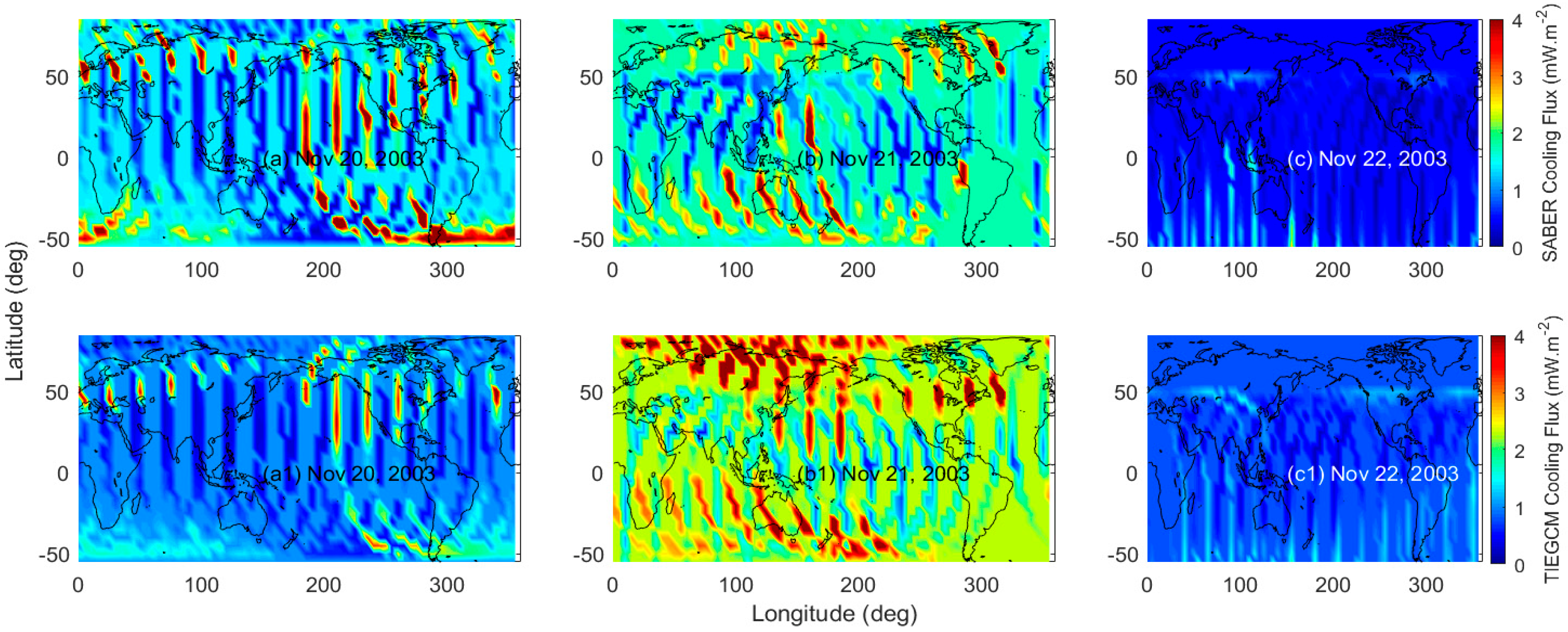
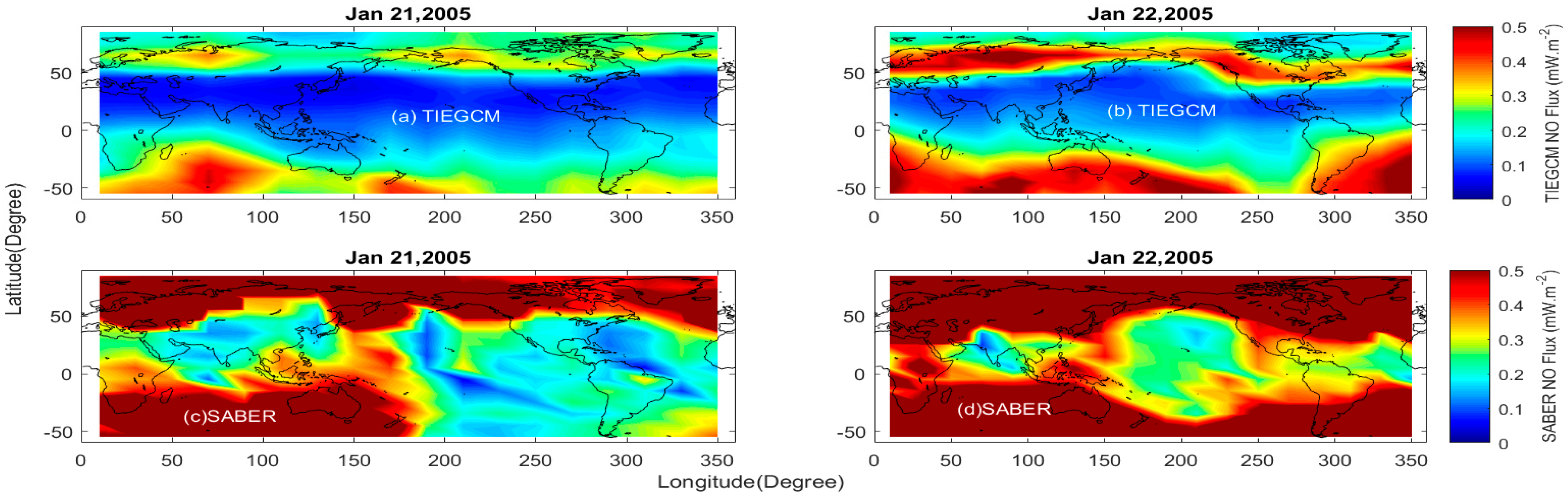
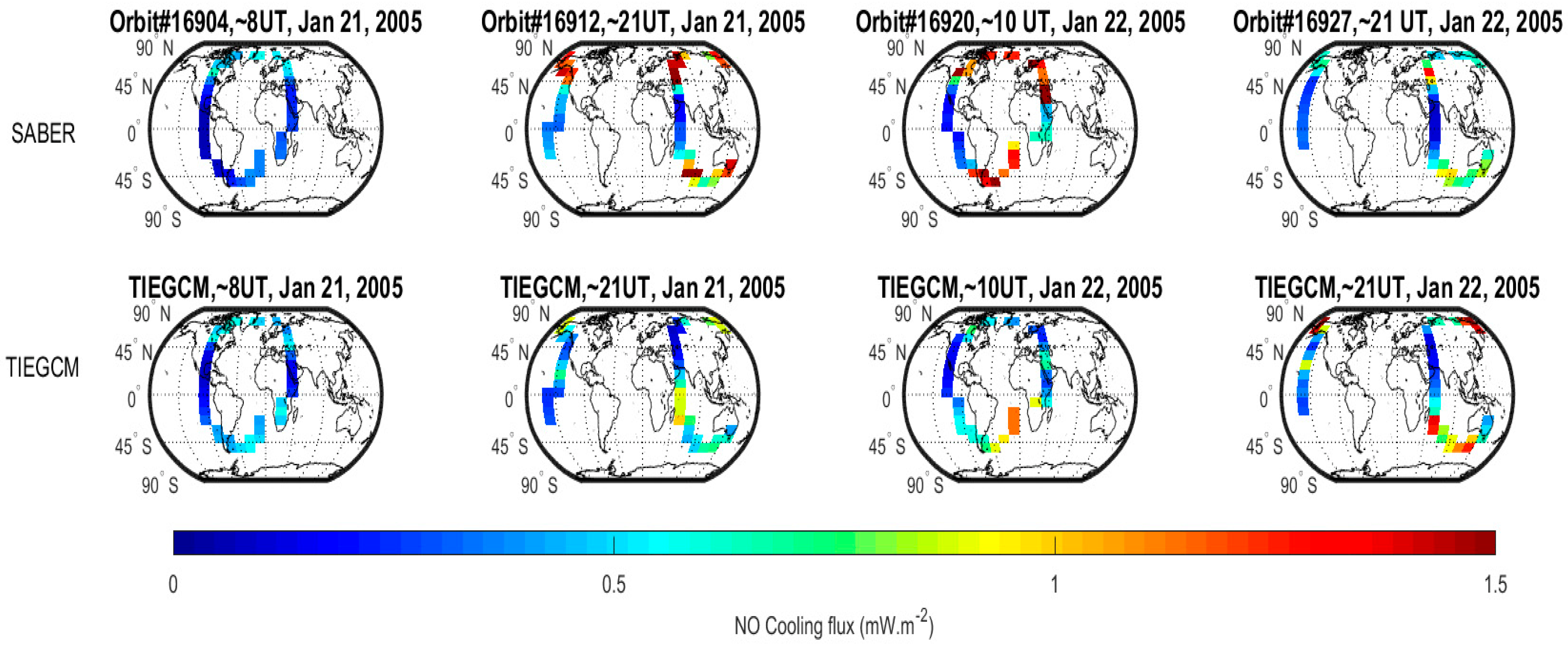
3.2. Latitude–Longitude Variation

The latitude–longitude cross-sectional view of the NO cooling flux during the storm event is shown in Figure 4. The cooling flux is binned into a 10° in latitude and 20° in longitude grid. It can be noticed that the TIEGCM simulation has relatively higher cooling flux in the high latitudes as compared with the low and equatorial regions. In addition, the cooling flux also increases during 22 January 2005 (Figure 4a,b). Similar enhancement is also noticeable in the satellite observations (Figure 4c,d). However, the satellite measurement is significantly higher than the model results all over the globe. It is to be noted that there are several studies on the comparison between TIMED-SABER measurement and TIEGCM simulations. Qualitatively the TIEGCM simulation can capture the observations. The earlier studies report that the TIEGCM model, as compared with observations, underestimates in the high latitude and overestimates in the low latitude regions [30,31,32,33,34]. However, an extreme underestimation by approximately one-fourth (¼) of the observation is noticed both in the high and low latitude regions. It is obviously an exceptional case where the TIEGCM simulation could not capture the observations.
In order to understand the local variation, we studied orbit-wise comparison between the model result and observation, which is shown in Figure 5. We selected four orbits; one orbit (#16904) corresponds to pre-storm period and the other three are during storm. The TIEGCM simulation results agree very well with the observation during quiet period (Orbit #16904, approximately 8 UT on 21 January 2005), with a slightly higher cooling flux over the southern hemisphere, particularly over the African and South American sectors. The cooling flux during the main phase of the storm at approximately 21 UT on 21 January is represented by Orbit #16912. The TIMED-SABER observation shows a strong intensification in the cooling flux, which can be clearly noticed above 40–45° latitude in both the hemispheres. The TIEGCM also exhibits an increase in the cooling flux. However, the model cannot capture the observation. Similar extreme underestimation in the modeled result can also be noticed for Orbit #16920. As the storm recedes, the SABER observed cooling also decreases. The TIEGCM simulation shows relatively higher value than the observations (Orbit #16927) during the post-storm period.
We also studied the latitudinal variation of NO cooling flux during this event by using both model and observation, as shown in Figure 6. We separated the latitudes into 30° bins. The dashed and the solid lines, respectively, represent the model simulation and observation results. The model result matches very well with the observation in the north hemisphere before the storm’s onset. On the other hand, it shows a relatively higher value than the observation in the southern hemisphere. As the storm arrives, the TIEGCM shows slight enhancement particularly in the latitude above ±60°, with maximum increase observed in the southern hemisphere. The TIEGCM does not show any significant variation in the latitude of 60–90°. However, a drastic increase is noticed in the TIMED-SABER satellite observations in all the latitude sectors. The relative change (%) in the latitudinal variation of NO cooling flux between model and observation is shown in Figure 6f. The relative increase in observed cooling flux is higher in the high latitude. The maximum relative enhancement is observed within 18 h of the onset. Further, the maximum enhancement of approximately 70% is observed in the 30–60° latitude region in the northern hemisphere. The enhanced flux sustains longer in the high latitude region as compared with the low latitudes.

4. Discussion

The TIEGCM model uses the formulation of Kockarts (1980) to calculate the cooling emission as discussed above. The production of NO cooling emission depends on the densities of atomic and molecular oxygen, nitric oxide, and the thermospheric temperature (see Equation (3)). The changes in these parameters would strongly dictate the variability in cooling emission. However, Murphy et al. (1975) [24] reported that the efficiency of energy transfer between v = 0 and v = 1 vibrational level by atomic oxygen is approximately 104–105 times higher than that by other neutral species. Consequently, the dependence of NO cooling emission on the molecular oxygen can be neglected.
The cooling emission is very sensitive to the temperature variation due to the exponential dependence [10,17]. We investigate the TIEGCM-model-calculated atomic oxygen, nitric oxide, and temperature variation to understand the extreme underestimation during this event. Figure 7a–f depict the TIEGCM simulated latitude–longitude cross-sections of the thermospheric temperature and densities of atomic oxygen and NO along the satellite orbit corresponding to the altitude of 130 km. The thermospheric temperature during 21 January 2005, and January 22, 2005, are, respectively, shown in Figure 7a,b. A global increase in the temperature structure can be observed during 22 January 2005, except near the 50–100° longitude region in the latitude of ± 50°. Equation (3) has only an exponential temperature dependence term. Other reaction rate coefficients are independent of temperature. It is to be noted that Sheng et al. (2017) [32] reported that the use of a temperature-dependent chemical reaction (in N ( 2 D ) + O 2 N O + O 2 ) proposed by Duff et al. (2003) [45] could be able to predict the recovery time neutral density more closely to the observations in the high latitude southern hemisphere. However, there was still a strong discrepancy in the low latitude and northern hemisphere. The atomic oxygen density during 21 January 2005, shows a strip of relatively higher magnitude in latitude below 50° in the northern hemisphere (Figure 7c). The high latitude region undergoes depletion, and no significant variation is observed in the equatorial region (Figure 7d). Maximum enhancement of approximately 20% is observed in the western longitude sector above approximately 50° latitude. The nitric oxide density on 21 January 2005, is relatively higher in the southern hemisphere and at the high latitude region above 50° in the northern hemisphere as compared with the equatorial region. Similarly, it also has higher magnitude in the eastern longitude sector as compared with the western longitude. The nitric oxide density undergoes a strong variation during storm period (Figure 7f). The nitric oxide density increases over the globe, and this increase is higher in the high latitude region. The NO cooling emission is directly affected by the NO molecules. On the other hand, the particle precipitation indirectly dictates the cooling by changing the production of molecular NO. The nitric oxide density is strongly modulated by the low energy particle precipitation [29,46,47,48,49,50,51,52]. The auroral electrons of energy 1–10 keV dissociates N2 molecule to create NO. The electrons of energy 0.1 keV can penetrate into the altitude of 230 km, whereas electrons of 10 keV energy can affect the altitude of 105 km. Similarly, the ion of energy 10 keV can reach up to the altitude of 120 km. The particle flux during 21–22 January is depicted in Figure 8. Both the electron and particle flux increase as the storm starts. Correspondingly, the increase in the nitric oxide during 22 January 2005, could be due to the particle (electron/ion) precipitation during 21 January 2005. The TIMED/GUVI observation of O/N2 ratio also shows an equatorward propagation during the storm period (Figure 9). This equatorward movement is due to well-known storm-time equatorward meridional wind. The O/N2 ratio is anti-correlated with the NO density on global scale [40,41]. The deposition of depleted O/N2 ratio into the mid–low latitude would further increase the NO density in these latitudes, which is clearly seen in the NO density increase. Another possibility is that the increase in the Joule heating rate due to increased convection velocity at high latitude is underestimated compared with the actual one. The convection velocity is roughly proportional to the solar wind velocity. The increase in the IMF |B| and solar wind velocity continues until approximately 30 h later (see Figure 2). Thus, the Weimer model might have underestimated the high-latitude convection and particle precipitation fluxes. It is because the Weimer model’s (1) calculation of the cross polar cap potential is relatively insensitive to the solar wind density, and (2) the electric field for solar wind speed > 900 km/s and (3) IMF > 20 nT can be unrealistic. We would like to emphasize here that although the TIEGCM simulation results exhibit an enhancement in the densities of atomic oxygen, nitric oxide, and temperature, the model severely underestimates the observed NO cooling emission. The TIEGCM is inadequate in predicting the observed cooling emission during this “anomalous” event. It could be due to the fact that the TIEGCM does not exhibit stronger temperature variation and the reaction rate coefficients are temperature-independent. However, more studies are needed to understand the TIEGCM’s underestimation during this event.

5. Conclusions

The thermospheric temperature increases significantly during geomagnetic storm events due to the solar energy deposition into the Earth’s high latitude region. The infrared radiative emission processes strongly regulate the thermospheric temperature particularly during geomagnetic disturbed events. Among the radiative coolants, the nitric oxide at 5.3 µm is the dominating cooling agent in the altitude of 100 to 300 km and is well known as the natural thermostat. We investigate the response of nitric oxide 5.3 µm emission during an anomalous geomagnetic storm of 21–22 January 2005, by using data from the TIEGCM simulation and the TIMED-SABER satellite observations. The peculiarity of this storm is that the main phase developed during the northward orientation of the z-component of the interplanetary magnetic field. The peak Dst index is observed to be −105 nT, with a long-lasting recovery phase. We compared the local and global variation between the model and observation results. Surprisingly, the model could not capture the observations. Although the model simulation results exhibit enhancements in the densities of atomic oxygen, nitric oxide, and temperature in-line with the DMSP observations of precipitating particle flux and GUVI O/N2 ratio during the storm event, the model underestimates by approximately one-fourth the observation value. More studies are needed to understand the inadequacy of the TIEGCM model results during anomalous storm periods.

Author Contributions

Conceptualization, T.B. and D.R.; methodology, T.B., D.R., Y.O. and V.S.; software, T.B.; validation, T.B.; formal analysis, T.B.; investigation, T.B., D.R. and Y.O.; resources, T.B.; data curation, T.B.; writing—original draft preparation, T.B. and D.R.; writing—review and editing, Y.O. and V.S.; visualization, T.B.; supervision, T.B. and Y.O.; project administration, T.B., D.R. and Y.O.; funding acquisition, T.B. and Y.O. All authors have read and agreed to the published version of the manuscript.

Funding

T. Bag is supported by Japan Society for the Promotion of Science (JSPS) postdoctoral fellowship for research in Japan, grant number: 22F32017. D. Rout acknowledges the support from Humboldt Research Fellowship for Postdoctoral Researchers (Humboldt foundation grants PSP D-023-20-001).

Data Availability Statement

All data used here are available on the public domain. The thermospheric cooling data are from the TIMED-SABER satellite observations (http://saber.gats-inc.com/data.php; accessed on 22 September 2022). The TIEGCM simulation results are obtained from NASA-CCMC (https://ccmc.gsfc.nasa.gov) archive Tikemani_Bag_092022_IT_4, accessed on 26 September 2022. Hemispheric power is from NOAA via ftp://ftp.swpc.noaa.gov/pub/lists/hpi; accessed on 19 October 2022. The particle flux data are obtained from DMSP satellite via the Madrigal database (http://cedar.openmadrigal.org/single, accessed on 26 September 2022). The magnetic and interplanetary magnetic field data are from NASA’s OMNIweb (https://omniweb.gsfc.nasa.gov/), accessed on 22 September 2022.

Acknowledgments

We thank the SABER, GUVI, DMSP, NOAA, and OMNI teams for providing the data.

Conflicts of Interest

The authors declare no conflict of interest.

References

  1. Tsurutani, B.T.; Gonzalez, W.D. The causes of geomagnetic storms during solar maximum. Eos Trans. AGU 1994, 75, 49–53. [Google Scholar] [CrossRef]
  2. Tsurutani, B.T.; Gonzalez, W.D.; Tang, F.; Akasofu, S.I.; Smith, E.J. Origin of interplanetary southward magnetic fields responsible for major magnetic storms near solar maximum (1978–1979). J. Geophys. Res. 1988, 93, 8519–8531. [Google Scholar] [CrossRef]
  3. Du, A.M.; Tsurutani, B.T.; Sun, W. Anomalous geomagnetic storm of 21–22 January 2005: A storm main phase during northward IMFs. J. Geophys. Res. 2008, 113, A10214. [Google Scholar] [CrossRef] [Green Version]
  4. Kozyra, J.U.; Liemohn, M.W.; Cattell, C.; De Zeeuw, D.; Escoubet, C.P.; Evans, D.S.; Fang, X.; Fok, M.C.; Frey, H.U.; Gonzalez, W.D.; et al. Solar filament impact on 21 January 2005: Geospace consequences. J. Geophys. Res. Space Phys. 2014, 119, 5401–5448. [Google Scholar] [CrossRef] [Green Version]
  5. Sahai, Y.; Fagundes, P.R.; De Jesus, R.; De Abreu, A.J.; Crowley, G.; Kikuchi, T.; Huang, C.S.; Pillat, V.G.; Guarnieri, F.L.; Abalde, J.R.; et al. Studies of ionospheric F-region response in the Latin American sector during the geomagnetic storm of 21–22 January 2005. Ann. Geophys. 2011, 29, 919–929. [Google Scholar] [CrossRef] [Green Version]
  6. Manchester, W.B., IV; Kozyra, J.U.; Lepri, S.T.; Lavraud, B. Simulation of magnetic cloud erosion during propagation. J. Geophys. Res. Space Phys. 2014, 119, 5449–5464. [Google Scholar] [CrossRef] [Green Version]
  7. Manchester, W.B., IV; Ridley, A.J.; Gombosi, T.I.; Dezeeuw, D.L. Modeling the Sun-to-Earth propagation of a very fast CME. Adv. Space Res. 2006, 38, 253–262. [Google Scholar] [CrossRef]
  8. D’Uston, C.; Bosqued, J.M.; Cambou, F.; Temny, V.V.; Zastenker, G.N.; Vaisberg, O.L.; Eroshenko, E.G. Energetic properties of interplanetary plasma at the Earth’s orbit following the August 4, 1972 flare. Sol. Phys. 1977, 51, 217. [Google Scholar] [CrossRef]
  9. Kockarts, G. Nitric oxide cooling in the terrestrial thermosphere. Geophys. Res. Lett. 1980, 7, 137–140. [Google Scholar] [CrossRef]
  10. Mlynczak, M.; Martin-Torres, F.J.; Russell, J.M., III; Beaumont, K.; Jacobson, S.; Kozyra, J.; Lopez-Puertas, M.; Funke, B.; Mertens, C.; Gordley, L.; et al. The natural thermostat of nitric oxide emission at 5.3 µm in the thermosphere observed during the solar storms of April 2002. Geophys. Res. Lett. 2003, 30. [Google Scholar] [CrossRef] [Green Version]
  11. Barth, C.A. Nitric oxide in the lower thermosphere. Planet. Space Sci. 1992, 40, 315–336. [Google Scholar] [CrossRef]
  12. Gardner, J.L.; López-Puertas, M.; Funke, B.; Miller, S.M.; Lipson, S.J.; Sharma, R.D. Rotational and Spin-orbit distributions of NO observed by MIPAS/ENVISAT during the solar storm of October/November 2003. J. Geophys. Res. 2005, 110, A09S34. [Google Scholar] [CrossRef] [Green Version]
  13. Richards, P.G. On the increases in nitric oxide density at midlatitudes during ionospheric storms. J. Geophys. Res. 2004, 109, A06304. [Google Scholar] [CrossRef]
  14. Jones, M., Jr.; Forbes, J.M.; Hagan, M.E. Solar cycle variability in mean thermospheric composition and temperature induced by atmospheric tides. J. Geophys. Res. Space Phys. 2016, 121, 5837–5855. [Google Scholar] [CrossRef] [Green Version]
  15. Mlynczak, M. A comparison of space-based observations of the energy budgets of the mesosphere and troposphere. J. Atmos. Sol. Terr. Phys. 2002, 64, 877–887. [Google Scholar] [CrossRef]
  16. Yee, J.H.; Talaat, E.R.; Christensen, A.B.; Killeen, T.L.; Russell, J.M., III; Woods, T.N. TIMED instruments. Johns Hopkins APL Tech. Dig. 2003, 24, 156–164. [Google Scholar]
  17. Mertens, C.J.; Russell, J.M., III; Mlynczak, M.G.; She, C.Y.; Schmidlin, F.J.; Goldberg, R.A.; López-Puertas, M.; Wintersteiner, P.P.; Picard, R.H.; Winick, J.R.; et al. Kinetic temperature and carbon dioxide from broadband infrared limb emission measurements taken from the TIMED/SABER instrument. Adv. Space Res. 2009, 43, 15–27. [Google Scholar] [CrossRef] [Green Version]
  18. Mlynczak, M.G.; Hunt, L.A.; Marshall, B.T.; Martin-Torres, F.J.; Mertens, C.J.; Russell, J.M., III; Remsberg, E.E.; López-Puertas, M.; Picard, R.; Winick, J.; et al. Observations of infrared radiative cooling in the thermosphere on daily to multiyear timescales from the TIMED/SABER instrument. J. Geophys. Res. 2010, 115, A03309. [Google Scholar] [CrossRef]
  19. Hunt, L.A.; Mlynczak, M.G.; Marshall, B.T.; Mertens, C.J.; Mast, J.C.; Thompson, R.E.; Gordley, L.L.; Russell, J.M., III. Infrared radiation in the thermosphere at the onset of solar cycle 24. Geophys. Res. Lett. 2011, 38, L15802. [Google Scholar] [CrossRef]
  20. Roble, R.G.; Ridley, E.C.; Richmond, A.D.; Dickinson, R.E. A coupled thermosphere/ionosphere general circulation model. Geophys. Res. Lett. 1988, 15, 1325–1328. [Google Scholar] [CrossRef]
  21. Richmond, A.D.; Ridley, E.C.; Roble, R.G. A thermosphere/ionosphere general circulation model with coupled electrodynamics. Geophys. Res. Lett. 1999, 19, 601–604. [Google Scholar] [CrossRef]
  22. Heelis, R.A.; Lowell, J.K.; Spiro, R.W. A model of the high-latitude ionospheric convection pattern. J. Geophys. Res. Space Phys. 1982, 87, 6339–6345. [Google Scholar] [CrossRef]
  23. Weimer, D. Predicting surface geomagnetic variations using ionospheric electrodynamic models. J. Geophys. Res. 2005, 110, A12307. [Google Scholar] [CrossRef]
  24. Hagan, M.E.; Forbes, J.M. Migrating and nonmigrating tides in the middle and upper atmosphere excited by latent heat releases. J. Geophys. Res. 2002, 107, 4754. [Google Scholar] [CrossRef]
  25. Hwang, E.S.; Castle, K.J.; Dodd, J.A. Variational relaxation of NO(𝜈 = 1) by oxygen atoms between 295 and 825 K. J. Geophys. Res. 2003, 108, 1109. [Google Scholar] [CrossRef]
  26. Murphy, R.E.; Lee, E.T.P.; Hart, A.M. Quenching of vibrationally excited nitric oxide by molecular oxygen and nitrogen. J. Chem. Phys. 1975, 63, 2919. [Google Scholar] [CrossRef]
  27. Bag, T. Diurnal Variation of Height Distributed Nitric Oxide Radiative Emission During November 2004 Super-Storm. J. Geophys. Res. Space Phys. 2018, 123, 6727–6736. [Google Scholar] [CrossRef]
  28. Bag, T.; Li, Z.; Rout, D. SABER observation of storm-time hemispheric asymmetry in nitric oxide radiative emission. J. Geophys. Res. Space Phys. 2021, 126, e2020JA028849. [Google Scholar] [CrossRef]
  29. Bag, T.; Rout, D.; Ogawa, Y.; Singh, V. Distinctive response of thermospheric cooling to ICME- and CIR-driven geomagnetic storms. Front. Astron. Space Sci. 2023, 10. [Google Scholar] [CrossRef]
  30. Li, Z.; Knipp, D.; Wang, W.; Sheng, C.; Qian, L.; Flynn, S. A comparison study of NO cooling between TIMED/SABER measurements and TIEGCM simulations. J. Geophys. Res. Space Phys. 2018, 123, 8714–8729. [Google Scholar] [CrossRef]
  31. Li, Z.; Knipp, D.; Wang, W. Understanding the behaviours of thermospheric nitric oxide cooling during the 15 May 2005 geomagnetic storm. J. Geophys. Res. Space Phys. 2019, 124, 2113. [Google Scholar] [CrossRef]
  32. Li, Z.; Sun, M.; Li, J.; Zhang, K.; Zhang, H.; Xu, X.; Zhao, X. Significant Variations of Thermospheric Nitric Oxide Cooling during the Minor Geomagnetic Storm on 6 May 2015. Universe 2022, 8, 236. [Google Scholar] [CrossRef]
  33. Chen, X.; Lei, J. A numerical study of the thermospheric overcooling during the recovery phases of the October 2003 storms. J. Geophys. Res. Space Phys. 2018, 123, 5704. [Google Scholar] [CrossRef]
  34. Sheng, C.; Lu, G.; Solomon, S.C.; Wang, W.; Doornbos, E.; Hunt, L.A.; Mlynczak, M.G. Thermospheric recovery during the 5 April 2010 geomagnetic storm. J. Geophys. Res. Space Phys. 2017, 122, 4588–4599. [Google Scholar] [CrossRef] [Green Version]
  35. Rich, F.J.; Hardy, D.D.; Gussenhoven, M.S. Enhanced ionosphere-magnetosphere data from the DMSP satellites. EOS 1985, 66, 513. [Google Scholar] [CrossRef]
  36. Fuller-Rowell, T.J.; Evans, D.S. Height-integrated Pedersen and Hall conductivity patterns inferred from the TIROS/NOAA satellite data. J. Geophys. Res. 1987, 92, 7606–7618. [Google Scholar] [CrossRef]
  37. Emery, B.A.; Coumans, V.; Evans, D.S.; Germany, G.A.; Greer, M.S.; Holeman, E.; Kadinsky-Cade, K.; Rich, F.J.; Xu, W. Seasonal, Kp, solar wind, and solar flux variations in long-term single-pass satellite estimates of electron and ion auroral hemispheric power. J. Geophys. Res. 2008, 113, A06311. [Google Scholar] [CrossRef] [Green Version]
  38. Christensen, A.B.; Paxton, L.J.; Avery, S.; Craven, J.; Crowley, G.; Humm, D.C.; Kil, H.; Meier, R.R.; Meng, C.I.; Morrison, D.; et al. Initial observations with the Global Ultraviolet Imager (GUVI) in the NASA TIMED satellite mission. J. Geophys. Res. 2003, 108, 1451. [Google Scholar] [CrossRef]
  39. Strickland, D.J.; Meier, R.R.; Walterscheid, R.L.; Craven, J.D.; Christensen, A.B.; Paxton, L.J.; Morrison, D.; Crowley, G. Quiet-time seasonal behaviour of the thermosphere seen in the far ultraviolet dayglow. J. Geophys. Res. 2004, 109, A01302. [Google Scholar] [CrossRef]
  40. Zhang, Y.; Paxton, L.J.; Morrison, D.; Wolven, B.; Kil, H.; Meng, C.I.; Mende, S.B.; Immel, T.J. O/N2 changes during 1–4 October 2002 storms: IMAGE SI-13 and TIMED/GUVI observations. J. Geophys. Res. 2004, 109, A10308. [Google Scholar] [CrossRef]
  41. Zhang, Y.; Paxton, L.J.; Morrison, D.; Marsh, D.; Kil, H. Storm-time behaviours of O/N2 and NO variations. J. Atmos. Sol. Terr. Phys. 2014, 114, 42–49. [Google Scholar] [CrossRef]
  42. Foullon, C.; Owen, C.J.; Dasso, S.; Green, L.M.; Dandouras, I.; Elliott, H.A.; Fazakerley, A.N.; Bogdanova, Y.V.; Crooker, N.U. Multi-spacecraft study of the 21 January 2005 ICME: Evidence of current sheet substructure near the periphery of a strongly expanding fast magnetic cloud. Sol. Phys. 2007, 244, 139–165. [Google Scholar] [CrossRef]
  43. McKenna-Lawlor, S.; Li, L.; Dandouras, I.; Brandt, P.; Zheng, Y.; Barabash, S.; Bucik, R.; Kudela, K.; Balaz, J.; Strharsky, I. Moderate geomagnetic storm (21–22 January 2005) triggered by an outstanding coronal mass ejection viewed via energetic neutral atoms. J. Geophys. Res. 2010, 115, A08213. [Google Scholar] [CrossRef] [Green Version]
  44. Knipp, D.J.; Tobiska, W.K.; Emery, B.A. Direct and indirect thermospheric heating sources for solar cycles 21–23. Sol. Phys. 2004, 224, 495–505. [Google Scholar] [CrossRef]
  45. Duff, J.W.; Dothe, H.; Sharma, R.D. On the rate coefficient of the N(2D)+O2→NO+O reaction in the terrestrial thermosphere. Geophys. Res. Lett. 2003, 30, 1259. [Google Scholar] [CrossRef]
  46. Barth, C.A.; Mankoff, K.D.; Bailey, S.M.; Solomon, S.C. Global observations of nitric oxide in the thermosphere. J. Geophys. Res. 2003, 108, 1027. [Google Scholar] [CrossRef]
  47. Bailey, S.M.; Barth, C.A.; Solomon, S.C. A model of nitric oxide in the lower thermosphere. J. Geophys. Res. 2002, 107, A8. [Google Scholar] [CrossRef]
  48. Fang, X.; Randall, C.E.; Lummerzheim, D.; Wang, W.; Lu, G.; Solomon, S.C.; Frahm, R.A. Parameterization of mono energetic electron impact ionization. Geophys. Res. Lett. 2010, 37, L22106. [Google Scholar] [CrossRef]
  49. Fang, X.; Lummerzheim, D.; Jackman, C.H. Proton impact ionization and a fast calculation method. J. Geophys. Res. Space Phys. 2013, 118, 5369–5378. [Google Scholar] [CrossRef]
  50. Galand, M.; Roble, R.G.; Lummerzheim, D. Ionization by energetic protons in Thermosphere-Ionosphere Electrodynamics General Circulation Model. J. Geophys. Res. 1999, 104, 27973–27989. [Google Scholar] [CrossRef]
  51. Knipp, D.; Kilcommons, L.; Hunt, L.; Mlynczak, M.; Pilipenko, V.; Bowman, B.; Deng, Y.; Drake, K. Thermospheric damping response to sheath-enhanced geospace storms. Geophys. Res. Lett. 2013, 40, 1263–1267. [Google Scholar] [CrossRef]
  52. Lin, C.Y.; Deng, Y.; Knipp, D.J.; Kilcommons, L.M.; Fang, X. Effects of energetic electron and proton precipitations on thermospheric nitric oxide cooling during shock-led interplanetary coronal mass ejections. J. Geophys. Res. Space Phys. 2019, 124, 8125–8137. [Google Scholar] [CrossRef]
Figure 1. Comparison of TIMED/SABER and TIEGCM nitric oxide cooling flux during 20–22 November 2003 storm. The TIEGCM overestimates NO cooling emission during storm period.
Atmosphere 14 00556 g001
Figure 2. Solar wind parameters during 21–22 January 2005, storm. (a) IMF Bz, (b) B, (c) solar wind density, (d) solar wind speed, (e) dynamics pressure, and (f) Sym-H. The vertical redlines represent the time of sudden storm commencements.
Atmosphere 14 00556 g002
Figure 3. Temporal variation of (a) Joule heating Power, (b) NOAA-observed hemispheric power and (c) orbit-averaged NO cooling flux from the TIEGCM simulation and TIMED-SABER observations.
Atmosphere 14 00556 g003
Figure 4. Latitude–longitude cross-section of nitric oxide flux from (a,b) the TIEGCM simulation and (c,d) TIMED-SABER satellite observation.
Atmosphere 14 00556 g004
Figure 5. Orbit-wise comparison between (top) SABER observations and (bottom) model results.
Atmosphere 14 00556 g005
Figure 6. Latitudinal variation of cooling flux (ae) for different latitude regions and (f) relative (%) change with respect to SABER observations. The solid and dashed lines, respectively, represent the observation and model results.
Atmosphere 14 00556 g006
Figure 7. TIEGCM simulated latitudinal–longitude cross-section of (a,b) temperature, (c,d) atomic oxygen, and (e,f) nitric oxide density along SABER satellite track corresponding to 130 km.
Atmosphere 14 00556 g007
Figure 8. Temporal variation of DMSP particle precipitation during 21–22 January 2005.
Atmosphere 14 00556 g008
Figure 9. GUVI observations of O/N2 ratio during 21–22 January 2005.
Atmosphere 14 00556 g009
Disclaimer/Publisher’s Note: The statements, opinions and data contained in all publications are solely those of the individual author(s) and contributor(s) and not of MDPI and/or the editor(s). MDPI and/or the editor(s) disclaim responsibility for any injury to people or property resulting from any ideas, methods, instructions or products referred to in the content.

