Forecasting Air Quality in Tripoli: An Evaluation of Deep Learning Models for Hourly PM_2.5 Surface Mass Concentrations

Abstract

In this article, we aimed to study the forecasting of hourly PM2.5 surface mass concentrations in the city of Tripoli, Libya. We employed three state-of-the-art deep learning models, namely long short-term memory, gated recurrent unit, and convolutional neural networks, to forecast PM2.5 levels using univariate time series methodology. Our results revealed that the convolutional neural networks model performed the best, with a coefficient of variation of 99% and a mean absolute percentage error of 0.04. These findings provide valuable insights into the use of deep learning models for forecasting PM2.5 and can inform decision-making regarding air quality management in the city of Tripoli.

1. Introduction

Environmental pollution has, for decades, changed climate and weather conditions. Moreover, the Earth’s system, which contains land, water, and air, is affected by pollution. The most serious pollution is air pollution, which affects every organism on the planet. Furthermore, the air works as an envelope of chemicals that protect the earth. For this reason, air pollution is seen by many as one of the main concentrations and greatest challenges the world has faced so far [1].

Pollutants are compounds floating in the air that are liquid, solid, gaseous, radioactive, or microbiological. The pollutants can be divided into two categories, human activities, and natural sources. Human sources are connected to industries, transportation, agriculture, and waste incineration in addition to some natural resources [2] and cultural resources [3]. Air pollution is one of the greatest causes of death in our world, and, as evidence of that, many dangerous diseases are caused by air pollution [4]. For example, heart disease, cancer, and chronic disease [5].

In 2020, air pollution was responsible for roughly 3.2 million fatalities per year, including over 237,000 deaths of children under the age of five [6]. Air pollution is regarded as one of the primary causes of global problems. Carbon monoxide, hydrocarbons, and carbon dioxide are the most common pollutants found in the air. Although it does not directly harm human health as a result of pollution, it acts as a greenhouse gas [7] that traps heat on Earth, resulting in global warming [8]. The best example is particulate matter (PM), which has an aerodynamic diameter of 10 (PM₁₀) or less and a diameter of 2.5 or less (PM_2.5). PM is a combination of solid particles and liquid droplets present in the atmosphere. These particles can include a variety of materials such as dirt, dust, soot, smoke, and pollens. Dust particles can be both natural and manmade and can vary in size from larger particles that can be seen with the naked eye to smaller particles that can only be detected using specialized instruments. The particle size is significant because smaller particles may penetrate deeper into the lungs and do more damage to human health. Long-term particulate matter exposure may cause a number of respiratory and cardiovascular disorders, as well as increase the chance of early mortality. Both are harmful to human health, however, it is more dangerous since it can enter the bloodstream and cause a variety of dangerous diseases, including heart and lung disease. Air pollution results in diseases, which make our lives shorter and make those still alive unhappy and suffer. That is why we should stop air pollution or reduce it, at least to reduce the associated diseases [4].

As an example of air pollution occurrence, in this study, we will consider the air pollution in Tripoli, the capital of Libya, which is located between latitude 32.87222 north and longitude 13.19611 east. Economically, Libya depends on fossil fuels, petroleum, and natural gas, and 100% of the population can get drinkable water and electricity easily [9]. Libya, like many other countries, suffers from air pollution caused by natural sources or human activities, such as transportation. Due to a lack of public transportation, the number of private vehicles increases, causing air pollution and contributing to climate change and global warming. In the crude oil refinery industries, Libya has five domestic refineries, Ras Lanuf export refinery, Al Zawiya refinery, Tobruk refinery, Brega refinery, and Sarir refinery. Refinery industries are the main source of atmospheric emissions of pollutants. The petrochemical industry produces products such as naphtha and natural gas. The steel and iron industry causes significant impacts on the environment due to the pollutants SO₂, CO, H₂S, PM, acids, benzene, phenol, salts, and grease residues. Cement industries and energy generation damage the environment, since the majority of Libya’s electricity is generated from polluting or nonrenewable sources such as natural gas and fossil fuel. Generally, in Libya, dust storms impact the environment, damage crops, reduce the fertility of the soil, damage the telecommunication and mechanical system, cause dirt and air pollution, and even airport shutdowns in some cases, and cause an increase in respiratory disease and other diseases [10].

Sandstorms aid in the transport and formation of PM. It is critical to model and estimate the quantities carried by the sand so that PM can be modeled, and the consequences can be considered. The frequency of dust storms in Libya reaches its maximum during the months of March, April, and May. During this period, the dust is moved by winds from the south to the west (as far as Tripoli) and east due to the strong movements in the desert depression. The dust particles are very small, which leads to very high concentrations of PM_2.5 and PM₁₀. The primary goal of this study is to model and forecast PM_2.5 levels derived from dust for the period between March and May.

Forecasting was done in this study using deep learning techniques, which are a subset of machine learning. We concentrated on two types of deep learning techniques in particular: convolutional neural networks (CNN) and recurrent neural networks (RNN). Deep learning is a powerful technique for time series analysis, as it can handle large amounts of data and extract meaningful features from it. One popular approach is to use long short-term memory (LSTM) network and gated recurrent unit (GRU), which are designed to handle sequential data. These networks can be trained to identify patterns and trends in the time series data and can be used for tasks such as forecasting, anomaly detection, and trend analysis.

1.1. Literature Review

Air pollution has recently become one of the world’s most prominent challenges. According to the World Health Organization (WHO), approximately 2.4 billion people are at risk of being exposed to high levels of air pollution, and ambient and household pollution causes seven million premature deaths each year [11]. It is recognized that air pollution could be ambient (outdoor) air pollution [12] or household air pollution [13]. Furthermore, it is believed that the quality of indoor air is worse than the quality of outdoor air, and it is estimated that the levels of pollutants in indoor air are nearly two to five times higher than the levels of pollutants in outdoor air, and in some cases exceed 100 times, as stated in [14].

A literature evaluation on air pollution may be categorized into three sections. To begin, certain research, depending on whether they investigate the association between pollutants and meteorological factors or the causes of air pollution, Second, several researchers have shown a link between pollution and a variety of health indicators. Finally, the third group focuses on air pollutants forecasting. In this subsection, we will be focusing on the third category.

Generally, linear regression methods are known as “simple machine learning algorithms.” Due to their simplicity, many publications by many researchers, such as [15] in 2018, focused on their applications in many fields. Also, [16] in 2020 examined the dataset collected monthly from Ankara between the period of Jan. 1993 and Dec. 2017, and the data was examined by a periodogram-based time series, and the periodic components were modeled by harmonic regression setup using the inherent dynamics of a time series. The study of [17] investigated the periodicity of daily particulate matter in 2020 in London, using data collected in the 2014–2018 period. The stationarity of the investigated data was checked by periodogram based on unit test roots, and it was found that harmonic regression works well in forecasting daily and monthly data averages. In Indonesia, the aerosol optical thickness was forecasted by [18] using a linear resolution model using MIRS sensors.

The authors of [19] utilized machine learning to forecast concentrations over time. They also used the Dickey–Fuller test (ADF) to determine whether the data was stationary before applying Savitzky–Goloy polynomial filters to achieve weekly and monthly decompositions for comparison, forecasting, and air pollution issues. In 2018 [20], a study in Malaysia was conducted to measure concentration using two models: regression with time series error and multiple linear regression, and 17% of the mean absolute error is calculated. In 2021, [21] began their analysis by testing the stationary of the data, followed by a time series model and periodogram-based unit root. They calculated the periodogram of the time series and discovered that 12 months and 240 months were significant. Applied regression models and artificial neural networks are used by [22] to forecast concentrations, while [23] forecasted in a short period by using multivariate linear regression. The location of the used data was Beijing, China, in 2018.

Machine learning and deep learning are important in many fields. Deep learning is part of the family of machine learning methods that are based on artificial neural networks. In 2022, [24] predicted daily data using a CNN+LSTM hybrid neural network model. The authors discovered that CNN+LSTM forecasting had error and bias around 1.51 and 6.46 times less than those of the three-dimensional chemistry transport model (3D-CTM) simulation, respectively, and that its accuracy was 1.10–1.18 times higher than the 3D-CTM. In 2020, hourly observations of concentrations in various regions were forecast by [25] by applying regression and time series analysis, depending on some factors such as the temperature of the atmosphere, wind speed, and pressure. Selected models such as regression model (Lasso), elastic net, random forest, decision tree extra-tree regression, RF-AdaBoost, XGBoost, and DT-AdaBoost were used to compare with the used model ET+AdaBoost using metrics such as mean absolute error and root mean squared error. The highest values of mean absolute error and root mean squared error were 22.18 and 38.13, respectively, with ET+AdaBoost having the highest of 0.92. An improved deep learning model as a predictor for daily observations is being continued by [26]. The effect of the density of sites and wind was considered for air pollution concentration by the weighted long short-term memory neural network (WLSTME). The performance of the proposed model, WLSTME, was measured by the scientific metrics root mean squared error, mean absolute error, and correlation coefficient as follows: 40.67, 26.10, and 0.59, respectively.

Also, [27] used machine learning to assess the impact of traffic on air pollutants; the methodology included artificial neural networks, boosted regression trees, and support vector machines. They thought the machine learning model worked very well to predict concentrations by using the R value as a metric, which was calculated as 0.8. The particular matter is modelled by [28] using five different methodologies. Metrics such as the coefficient of determination, mean absolute error, and mean squared error were used to compare the methods. The hybrid model had the best performance.

Other recent studies on modeling air pollution are [29,30,31,32,33,34,35]. An LSTM model based on principal component analysis (PCA) and attention mechanism (attention) was constructed by [29], which first used PCA to reduce data dimension, eliminate the correlation effect between indicators, and reduce model complexity, and then it uses the extracted principal components to establish a PCA-attention-LSTM model. To forecast the PM_2.5 concentration, simulation experiments were run using air pollutant data, meteorological element data, and working-day data from five cities in Ningxia from 2018 to 2020. The PCA-attention-LSTM model is compared to the support vector regression (SVR), AdaBoost, random forest (RF), BP neural network (BPNN), and LSTM models. The findings indicate that the PCA-attention-LSTM model is the best.

The goal of [30] was to determine the best geographical representation of PM_2.5, relative humidity, temperature, and wind speed in a Cartagena, Colombia metropolitan area. Empirical Bayesian kriging regression prediction was used to account for wind impacts. The use of these interpolation approaches defined the sections of the city that exceeded the acceptable limits of PM_2.5 concentrations and characterized three major meteorological variables in a continuous fashion on the surface. The main aim of [31] is to assess the mass concentration of different size-resolved particulate matter in the Wieliczka Salt Mine in southern Poland, compare it to the concentrations of the same PM fractions in the atmospheric air, and estimate the dose of dry salt aerosol inhaled by mine visitors.

The article [32] investigates the geographical and temporal dependency of PM_2.5 at the city level in China utilizing a three-year (2015–2017) dataset employing spatial statistics and time series analysis. Then, the authors offer a novel local regression model, multiscale geographically weighted regression (MGWR), on which [32] to quantify the effect of PM_2.5. To account for both spatiotemporal dependency and geographical variability, a spatiotemporal lag is built and incorporated into MGWR. The outcomes of MGWR are thoroughly compared to those of ordinary least squares and spatially weighted regression. The experimental findings reveal that PM_2.5 is spatially and temporally autocorrelated.

The authors of study [33] used a hybrid methodology that included integrated variable selection, autoregressive distributed lag, and the deletion of multiple collinear variables to reduce variables, and then applied six intelligent time series models to forecast the concentrations of the top three pollution sources. The authors gathered two air quality datasets from traffic and industrial monitoring sites, as well as meteorological data, to assess and compare their findings. The findings suggest that an RF based on key factors has higher classification metrics. A complete air quality model, particulate matter source apportionment technology, and monitoring data were employed in the research [34] for Beijing. The paper [35] describes the general observing system simulation experiments framework developed to aid in air quality forecasting, as well as the specifics of its constituent components. It also shows case study results from Northeast Asia and the potential benefits of new observation data scenarios on PM_2.5 forecasting skills, including PM data from 200 virtual monitoring sites in the Gobi Desert and nonforested areas of North Korea.

1.2. The Aime of the Study

In this study, we will compare the forecasting performance of deep learning architecture using PM_2.5 data. The hourly data originates from National Aeronautics and Space Administration (NASA) open data sources [11]. Given the background established in the literature review section, the following contributions to the literature may be listed. Deep learning technology is used to estimate and forecast Libya’s hourly PM concentration with amazing accuracy. The suggested model is of the univariate kind, which indicates that it simply makes use of time series data. It saves computation cost and effort by making accurate forecasting using just its own lags. The forecast models are rigorously tested and compared to various deep-learning approaches and hyperparameter settings.

The remainder of this paper is organized as follows: section two offers the theoretical background for the approaches employed. Section three is devoted to data and analysis. The discussion is covered in section four. Finally, section five concludes the study.

2. Methodology

The algorithms and performance metrics that are used throughout the rest of the article will be given in this section. We follow the methodology of [36]. The main difference between the methodology of [36] and this study is the following. In this research, forecasting for the short-term was generated using specific RNN and CNN. However, in the other study, forecasts for the short term and medium term were generated. In addition, although the research [36] used daily data, this study made use of data on an hourly basis. Since the quantity of power generated daily is derived by the aggregating of hourly data, it is not affected by time and season as much as the amount of particular matter observed hourly.

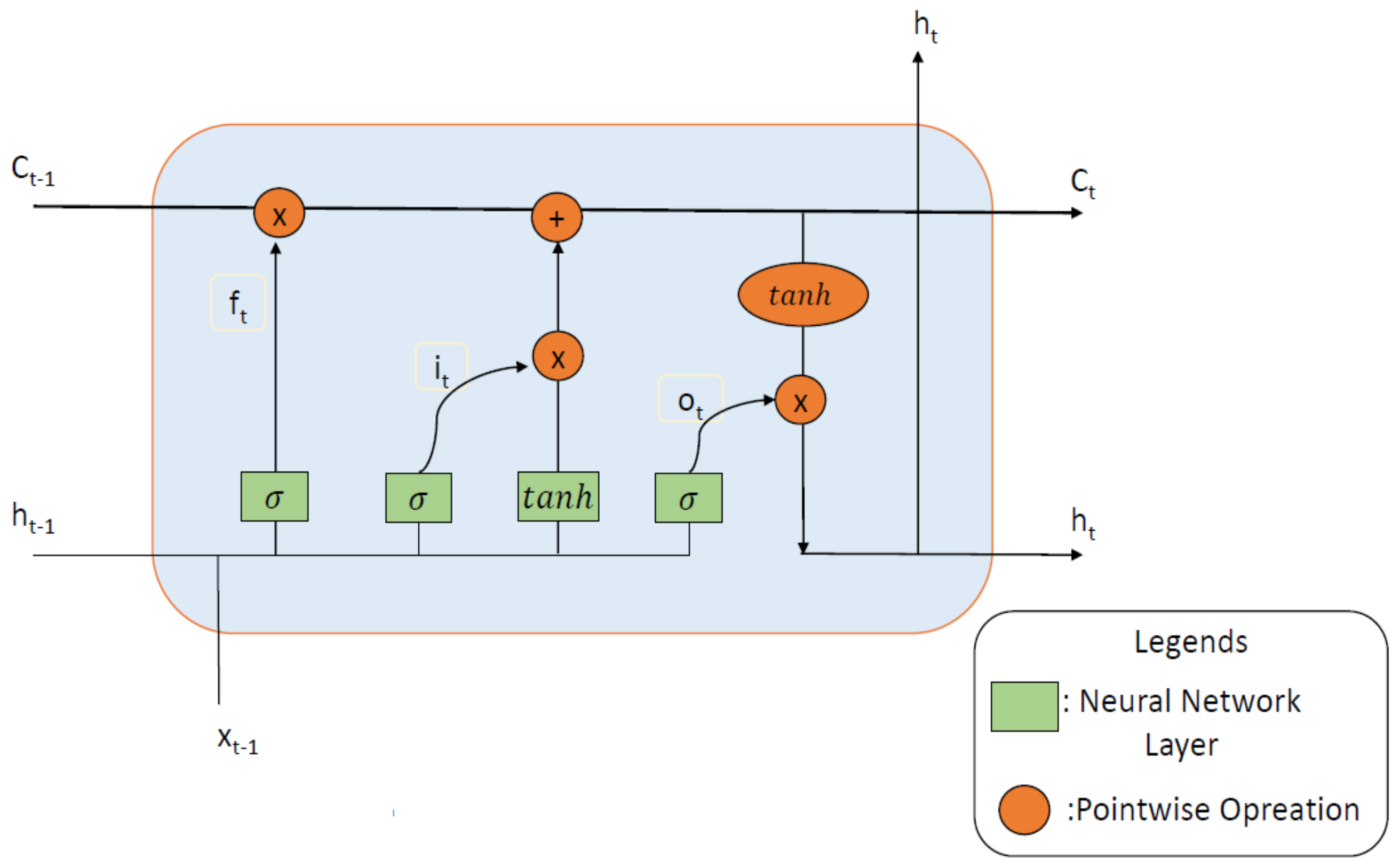
2.1. Long Short-Term Memory

The goal of the deep learning models known as feedforward networks is to approximate a specific set of functions. The algorithm is a powerful tool for predicting binary output, real-valued output, or both by practicing on examples and learning from those practices. This is an algorithm for learning via supervision. The model’s architecture consists of the input layer, hidden layer(s), and output layer. If the neural network in question does not have any hidden layers, we refer to it as a perceptron. On the other hand, if it does contain a significant number of hidden layers, we call it a multilayer feedforward network. Each layer has its own set of neurons. Neurons are the computational units that are found in the hidden layer. They are responsible for modifying the data that was input or pulsed by employing an activation function. Nonlinearity may be seen in the vast majority of these activation functions. In order to pulse the information, weight is assigned to the connections that are present between each neuron layer. Training the network refers to the process of making adjustments to the weights with the goal of achieving the lowest possible values for various statistical cost functions. In these models, the information is traced from the input layers to the hidden layers and then from the hidden layers to the output layers. There is no fast travel available between the levels. When processing time-series data at time t, the activation of a hidden layer ($h_t$) can be expressed as $h_t={\phi }_h\left(W_h{x}_t+b_h\right)$ where ${\phi }_h$ represents activation functions such as hyperbolic tangent, rectified linear unit (ReLU) or sigmoid function, and $W_h$, $x_t$, and $b_h$ represent the weight function, input, and bias, respectively [36].

Forecasting is the process of applying output activation functions to the weighted sum of the activation functions obtained from the hidden layers in the neural networks. This is expressed as ${\widehat{y}}_t={\phi }_h\left(W_h{x}_t+b_h\right)$, where ${\widehat{y}}_t$ represents the forecasted outcome [37]. There are no feedback links in this configuration. If the model has feedback connections, they are referred to as RNN [36].

The representation of sequential data, such as time series, text, and pictures, is a typical application for RNNs, which are a kind of neural network. They are networks that include loops that make it possible for the information to remain in the network for an extended period of time. It makes it possible to use outputs instead of inputs while still concealing the state of the system. To put it another way, the network has feedback loops that are capable of storing data from previous stages and may be used in the process of forecasting. One way to conceptualize an RNN is as a collection of numerous clones of the same network, each of which transmits a message to a successor in the network. The issue of vanishing gradients is a challenge that RNN has to deal with. The authors of [38] provide an innovative approach to resolving this issue. An extension of RNN is known as LSTM. It is a kind of RNN that is capable of learning about long-term partnerships due to the fact that it is able to learn about long-term dependency [36]. Figure 1 displays a depiction of an LSTM algorithm.

When dealing with LSTMs, the problem of long-term reliance is circumvented on purpose. They do not need to put any effort into developing their long-term memory since it is a trait that comes naturally to them. As can be seen in Figure 1, LSTM makes use of a new parameter denoted by the $c_t$. This parameter represents the memory cell and is responsible for encoding information up to the current time. The equations for the three gates are as follows: $i_t,f_t,$ and $o_t$. These gates are respectively known as the input gate, forget gate, and output gate. The three gates’ equations are as follows:

$$i_t=\mathrm{sigmoid}\left(V_i{h}_{t-1}+U_i{x}_t+b_i\right),$$

(1)

$$f_t=\mathrm{sigmoid}\left(V_f{h}_{t-1}+U_f{x}_t+b_f\right),$$

(2)

$$o_t=\mathrm{sigmoid}\left(V_o{h}_{t-1}+U_o{x}_t+b_o\right).$$

(3)

The rest of the updating equations are

$$c_t=f_t\ast c_{t-1}+i_t\ast d_t,$$

(4)

$$h_t=o_t\ast \tanh \left(c_t\right).$$

(5)

Component-wise multiplication is represented by the symbol * while $V$ and $U$ are the weights and $b_o$ represents the bias term. The input gate chooses the data that will be added to the cell, the forget gate chooses the data that will be forgotten, and the output gate chooses the data from the cell that will be used as input in the previous operation. The information is acquired by the first forget gate at epoch t as a function of the input $x_t$ and the preceding hidden layer $h_{t-1}.$ If the value of the forget gate is somewhat near to one, the information stored in the most recent memory cell, $c_{t-1}$, will be kept. In such a case, the data will be deleted. After that, the newly discovered information is combined with the previously known concealed state in order to generate the input gate $i_t$. In order to construct a new computer, it is first transformed into a memory cell $c_{t-1}$. If not, the data is erased.

Second, the input gate is created by merging the new information with the previously hidden state. It is converted into a memory cell, which is subsequently converted into a new $c_t$. Finally, the output gate decides whether or not the information will be used to generate the next hidden state. First, the current and prior concealed state numbers are transmitted into the third sigmoid function. The new cell state produced by the cell state is then transmitted through the tanh function. The dot-product is calculated. The network determines which information the concealed state should convey based on the final value. This concealed condition is employed in the forecast. Further details about the algorithm’s architecture can be found in [39].

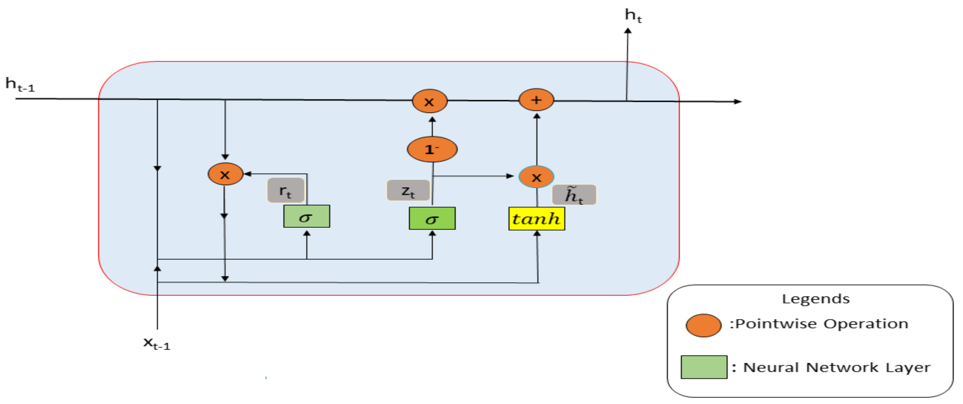
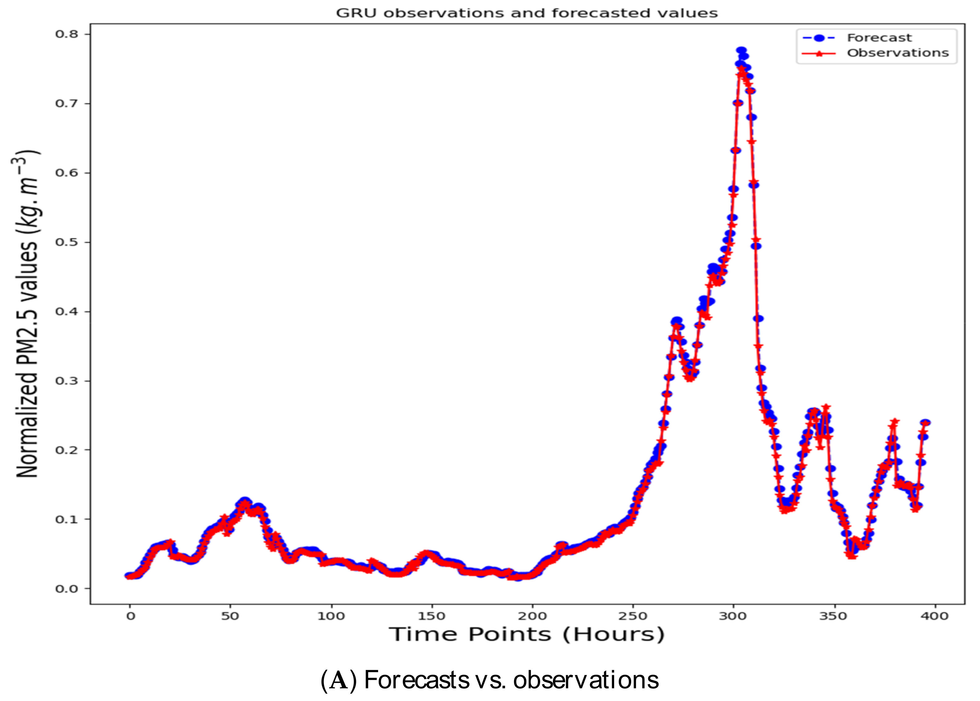
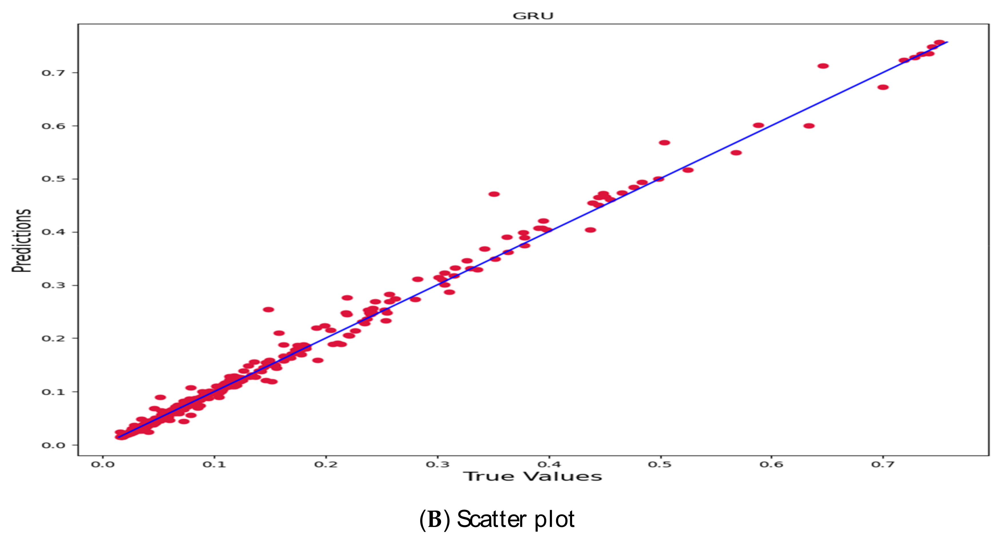
2.2. Gated Recurrent Unit

GRU, like LSTM, is proposed as a solution to the vanishing gradient problem. The LSTM extension is presented by [40]. The system’s recurrent units can handle long-term dependencies across a wide time span. The GRU algorithm couples the LSTM’s input and forgotten gates with a single update gate that functions as both the input and forgotten gates. Furthermore, the technique described by [40] combines cell states with concealed states. Figure 2 is the depiction of a GRU cell.

The architecture has been improved with the construction of two new gates. Reset gates and update gates are the two types of gates. The gates are used to store data and move it forward as needed. The model for GRU that may be written using the new gates is as follows:

$$r_t=\mathrm{sigmoid}\left(U_r{h}_{t-1}\ast x_t\right),$$

(6)

$$z_t=\mathrm{sigmoid}\left(U_z{h}_{t-1}\ast x_t\right),$$

(7)

$${\tilde{h}}_t=\tanh \left(U_t{r}_t{h}_{t-1}\ast x_t\right),$$

(8)

$$h_t=\left(1-z_t\right)h_{t-1}+z_t{h}_t.$$

(9)

Here, $h_t$ represents the hidden layer, $U$ represents the weights, $r_t$ symbols the reset gate and $z_t$ is the update gate. The reset and upgrade improve GRU’s performance while also saving time [40]. It is up to the reset gate and hidden layer to decide whether or not the former state’s information will be lost. The model’s overall performance and speed have improved significantly as a result of data parsing. For further indepth information, please see [40].

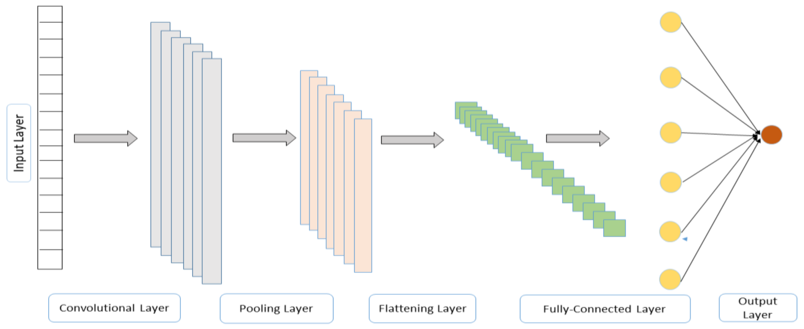
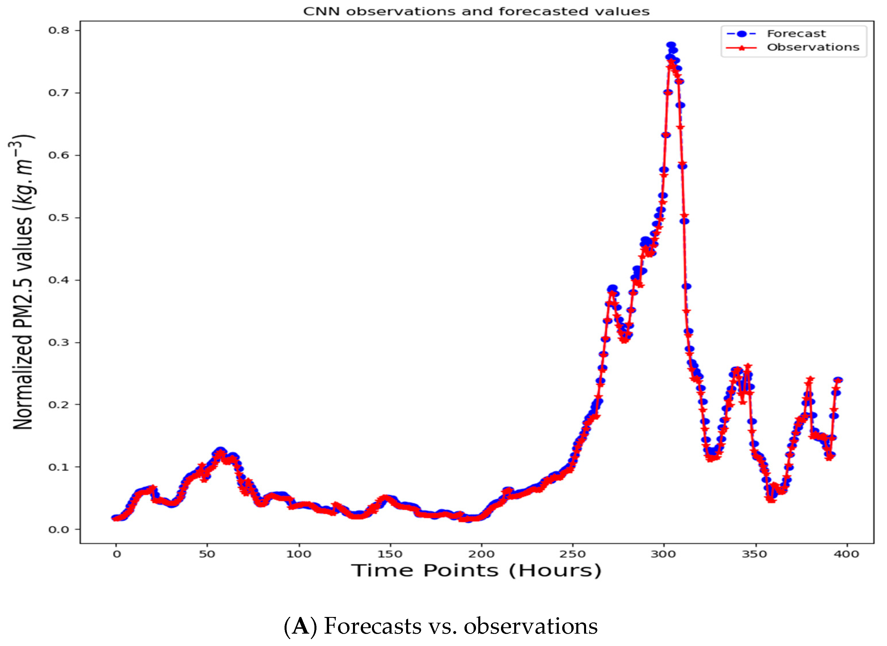
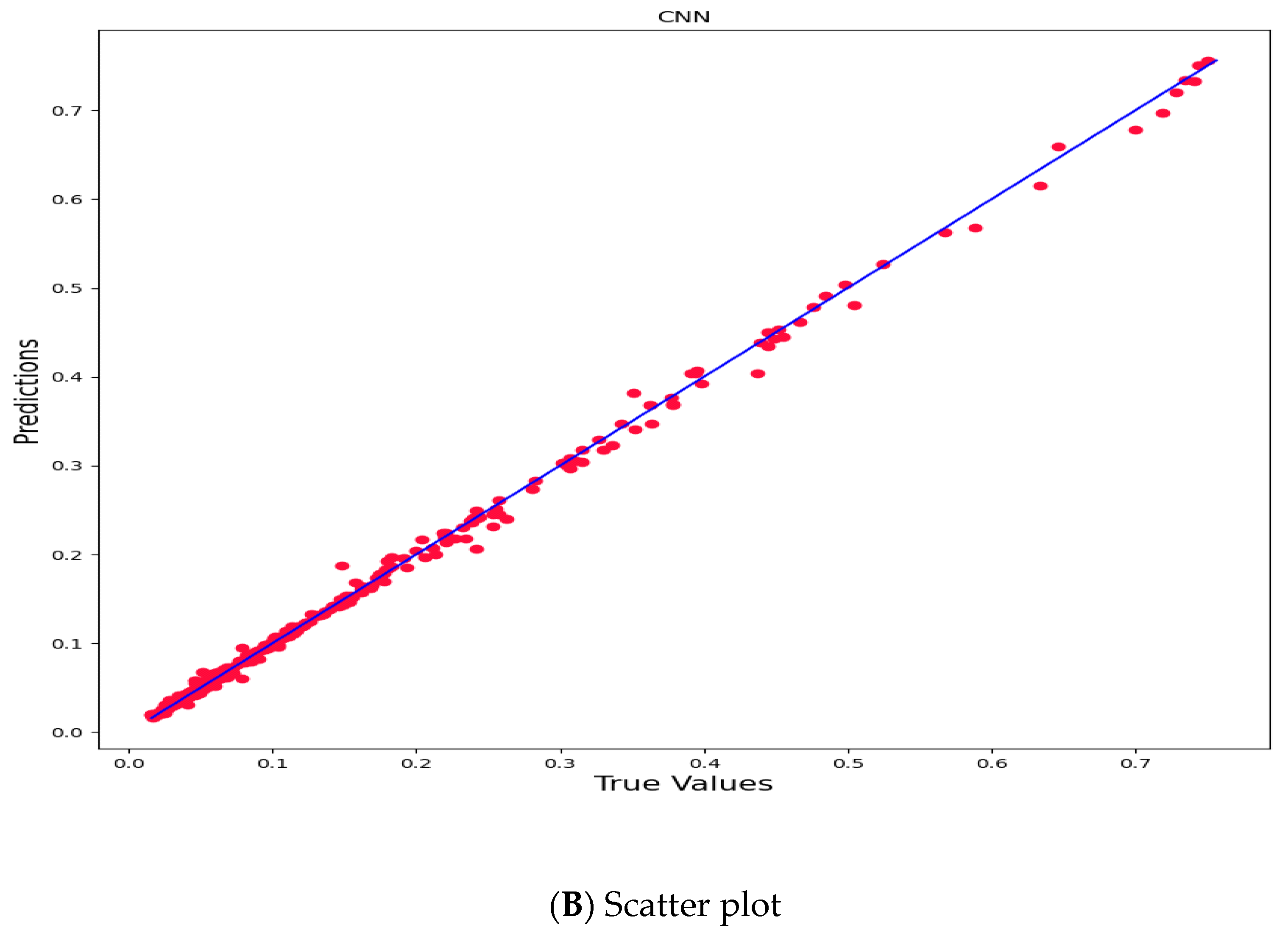
2.3. Convolutional Neural Networks

CNNs are specialized kinds of networks that perform extraordinarily well when dealing with data that is organized in a grid-like fashion, such as data on time series, photos, and videos that are streamed over the internet. The term “convolution” alludes to the mathematical operation that was the inspiration for the name of the network. CNN is responsible for the process of convolution. The subsequent levels are the pooling layer, the normalizing layer, and the completely connected layer. The major objective of each of these layers is either multiplication, dot product, or activation function. The first layer of a CNN is referred to as the convolutional layer. Before moving on to the next layer, convolutional layers integrate the input and output of the previous layer. This is analogous to the reaction that a cell in the visual cortex would have to a particular stimulus. Every single convolutional neuron will only process data pertaining to the receptive region it resides in. Even while fully connected feed-forward neural networks may be used to learn features and classify data, in certain cases it is not practicable to employ them with bigger inputs such as high-resolution photos due to their computational requirements. Pooling constitutes the second layer in the structure. Pooling layers reduce the amount of data that must be stored by combining the outputs of several neuron clusters from one layer into the input of a single neuron in the subsequent layer. This results in a smaller amount of data being stored. Since global pooling has an effect on each neuron in the feature map, one may deduce that it has an effect on all of the neurons. The maximum and the average are the two most popular applications of pooling. In the feature map, the max-pooling algorithm takes the largest possible value from each cluster of neurons. When using average pooling, all that is done is to take the mean of each cluster. The third layer is the layer that flattens the surface. It requires applying a one-dimensional vector transform to the pooled feature map that was created during the previous phase of pooling in order to convert it into a one-dimensional vector. This is done in order to prepare them for use as inputs in the thick layer at a later time. The final layer is the one that has all of its connections made. When all of the neurons in one layer are connected to all of the neurons in another layer, the neurons in both layers work together to provide meaning to the information they receive. A neural network comprised of many unique layers is referred to as a multilayer perceptron neural network. To categorize pictures, the flattened matrix passes through a fully linked layer [36]. Figure 3 depicts a CNN.

This type of network is usually used in image processing. The system perceives images as a two-dimensional grid of pixels. When applied to time-series data, this strategy is particularly successful. As a result, it treats time-series data as a one-dimensional space of space intervals. A more indepth examination of CNN can be found in [37].

2.4. Performance Metrics

We considered using five distinct criteria to assess the performance of the model in use. These measures are coefficient of determination (${\mathrm{R}}^2)$, mean absolute error (MAE), mean absolute percentage error (MAPE), root mean squared error (RMSE), and mean squared error (MSE).

The magnitude of the variations in the dependent variable that can be explained by an independent variable is measured by $R^2$. The following formula is used to compute it.

$$R^2=1-\frac{S{S}_{res}}{S{S}_{tot}},$$

(10)

where $S{S}_{res}={\sum }_{i=1}^n{\left(y_i-\widehat{f_i}\right)}^2={\sum }_{i=1}^n{e}_i{}^2$, it is known as the residual sum of squares and $\widehat{f_i}$ is the anticipated output. $S{S}_{tot}={\sum }_{i=1}^n{\left(y_i-\overline{y}\right)}^2$ is the total sum of the square and $\overline{y}$ is the mean of the observed data. It is used to assess a model’s goodness of fit. $R^2$ near to 1 indicate that the model has a very good forecasting performance.

MAPE is a measure of the accuracy of a forecasting method’s prediction that is used within the field of statistics. It is usual practice to represent accuracy as a ratio that is determined by a formula:

$$MAPE=\frac{1}{n}{\sum }_{i=1}^n\left|\frac{y_i-{\widehat{f}}_i}{y_i}\right|=\frac{1}{n}{\sum }_{i=1}^n\left|\frac{e_i}{y_i}\right|.$$

(11)

MSE is another kind of statistic that determines the level of discord between the intended result and the actual one. If the MSE is low, it indicates that the model’s ability to forecast accurately is high. The MSE may be determined by using:

$$MSE=\frac{1}{n}{\sum }_{i=1}^n{\left(y_i-{\widehat{f}}_i\right)}^2=\frac{1}{n}{\sum }_{i=1}^n{e}_i{}^2.$$

(12)

The MAE statistic quantifies the average magnitude error that occurs between the values of the target function and the observations produced by the function’s output. The model’s capacity for accurate prediction improves in proportion to the degree to which the magnitude changes. The formula for MAE is:

$$MAE=\frac{1}{n}{\sum }_{i=1}^n\left|y_i-{\widehat{f}}_i\right|=\frac{1}{n}{\sum }_{i=1}^n\left|e_i\right|.$$

(13)

RMSE is a measurement of the disparity between the values that are seen and the values that are projected by a model or estimator. The root mean square error, often known as the RMSE, is calculated by taking the square root of the second sample moment of the disparities that exist between the values that were predicted and those that were actually observed.

$$RMSE=\sqrt{MSE}=\sqrt{\frac{1}{n}{\sum }_{i=1}^n{\left(y_i-{\widehat{f}}_i\right)}^2=\frac{1}{n}{\sum }_{i=1}^n{e}_i{}^2.}$$

(14)

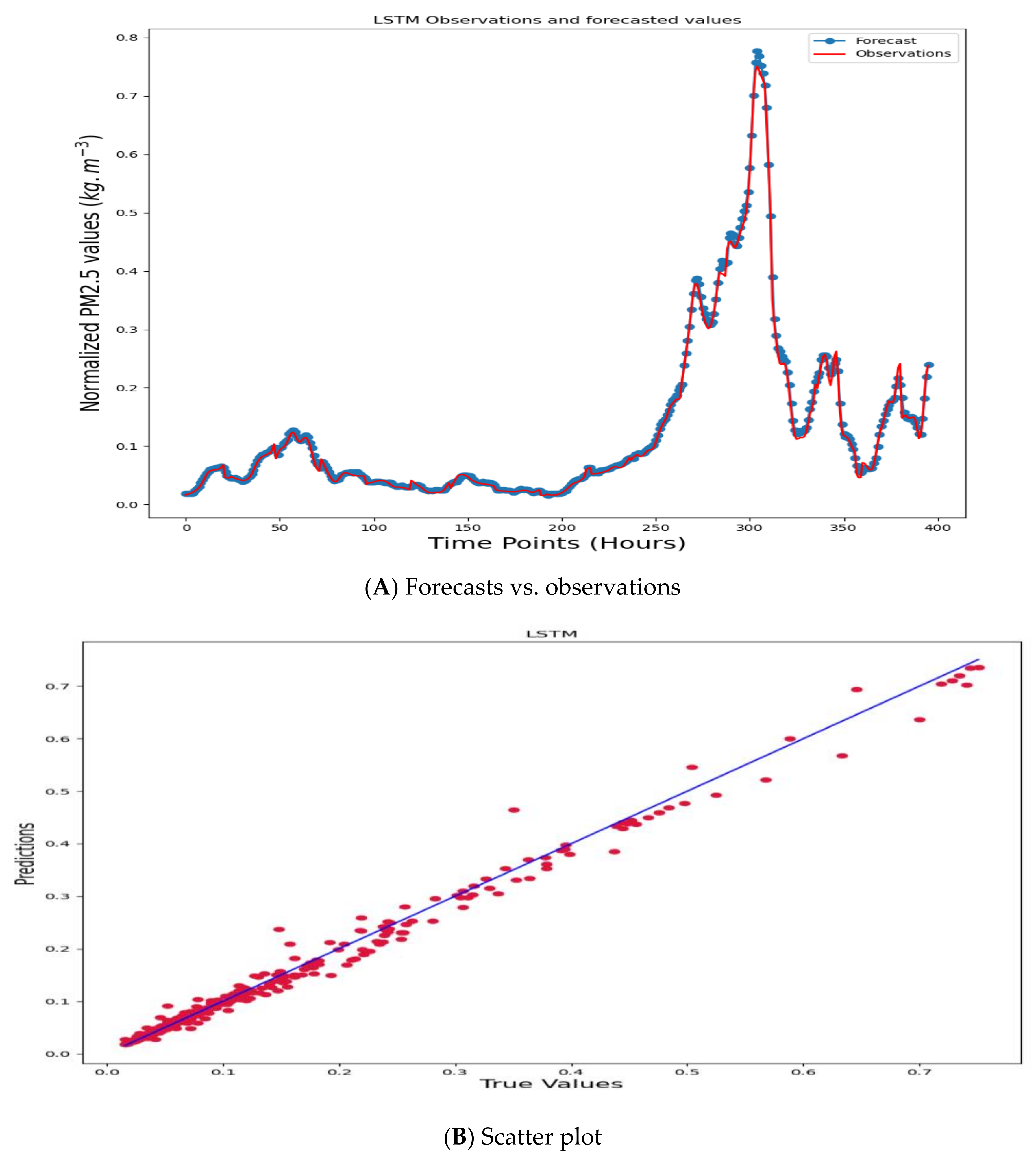
3. Empirical Evidence

There are two sources, as we mentioned before, natural and anthropogenic sources. We started with and focused too much on the last one since it is a common and friendly one for the reader, so it will be clear and the reader can get comprehensive information about what PM_2.5 is easily. As is well known, dust storms are one of the world’s most serious environmental issues. Furthermore, the Sahara Desert is the primary source of dust, accounting for 40–66% of the total, and dust is the primary source of PM_2.5 in Tripoli.

For example, the strongest and heaviest dust storm happened on 16 May 2017, which was almost the end of spring. That strong and dramatic dust storm was moving over Libya and caused a heavy, strong, and dangerous dust load. Since the dust contains PM_2.5 and other pollutants, it damages human health, buildings, vehicles, power poles, and trees throughout the center of the country (such as Tripoli) and even causes a total shutdown in airport operations. In Libya, dust storms are most common during the months of March, April, and May. Due to strong movements in the desert depression, the dust is moved by winds from the south to the west and east during this period. In this period, due to the dust particles, the concentrations of PM_2.5 and PM₁₀ are extremely high.

The data set of this study consists of its time average of PM_2.5 (dust surface mass concentration) gridded dataset of the Modern-Era Retrospective Analysis for Research and Applications Version 2 (MERRA-2) model with 0.5° × 0.625° spatial and hourly of Tripoli, Libya between the periods 1 March 2022, and 30 May 2022, with 2160 observations. The period between March and May is selected as the main investigation period since in the period the frequency of dust storms in Libya reaches its maximum level. The observations are measured in kg m⁻³. The sources of PM_2.5 are natural sources. The data set is obtained from open source data provider NASA [11]. More information can be obtained from [11]. When we investigate the data obtained from [11], it is seen that mass concentration levels are stable but high until May. In May the mass concentration increases and makes three pick points. In May also the average mass concentration level is higher than in the two considered months and the whole year.

Now, we scale the observations by utilizing min–max feature scaling which is

$$X_n=\frac{X-X_{min}}{X_{max}-X_{min}},$$

(15)

where $X$ represents the observation and $X_{min}$ and $X_{max}$ represent the lowest and highest values of the data set, respectively. In this study, we forecasted the next hour’s particulate matter concentration in a univariate sense. Thus we used different sizes of sliding windows to forecast the next hour’s concentration. The size of the window and segment keeps getting bigger until we reach the least error approximation at the number. The next segment is chosen after the first one has been chosen. The process is repeated until all of the time series data have been split into groups. In short, we use the input variables as the lag values of the variable that is $x_{t-T},x_{t-T-1},\dots ,x_{t-1}$. In each case, different lag lengths $\left(T\right)$ were used. Only lag values were employed in forecasting to anticipate the observation of $t$ hours, that is, it is targeted to calculate $\widehat{y_t}$ by only using the data itself. We fixed the size of the sliding window as 180 and investigated the behavior of the algorithms for different sizes of nodes to find the optimal node for the highest forecasting power. We have started our analysis with LSTM. In the algorithm, the structure is as follows. ReLU is used as the activation function, MSE is set as the loss function while an ADAM optimizer is utilized with an epoch size of 100. The lag length of the time series is taken as 180. The algorithms are trained for 80% of the whole data and the rest is used for testing the algorithm. The performance metrics for the LSTM are given in

Table 1. Performance metrics of LSTM for different number of nodes on the train set.

Number of Nodes	MAE	MSE	RMSE	R2	MAPE
10	0.0081	0.0002	0.0154	0.9885	0.0721
20	0.0081	0.0002	0.0146	0.9897	0.0746
30	0.0123	0.0003	0.0181	0.9843	0.1672
40	0.0157	0.0009	0.0307	0.9545	0.1253
50	0.0084	0.0003	0.0165	0.9868	0.0751
60	0.0119	0.0003	0.0167	0.9865	0.1741
70	0.0079	0.0002	0.0155	0.9884	0.0723
80	0.0091	0.0003	0.0168	0.9864	0.0877
90	0.0118	0.0004	0.0199	0.9807	0.1181
100	0.0094	0.0003	0.0184	0.9837	0.0887

.

According to each performance metric, the best result is obtained when the number of nodes is set to 20. In this case, the R² is calculated as 0.9897 and the MAPE is 0.0746. The graphs of the forecasted and observed values with their scatter plot is given in Figure 4. The observations and the forecasted values are given in Figure 4A while the scatter plot is given in Figure 4B.

We used ReLU as the activation function, as we did with LSTM. MSE is set as the loss function and the ADAM optimizer is utilized with an epoch size of 100. The lag length of the time series is taken as 180. The algorithms are trained for 80% of the whole data and the rest is used for testing the algorithm. The performance metrics for the GRU are given in

Table 2. Performance metrics of GRU for different number of nodes on the train set.

Number of Nodes	MAE	MSE	RMSE	R2	MAPE
10	0.0080	0.0024	0.0155	0.9885	0.0737
20	0.0069	0.0002	0.0135	0.9912	0.0602
30	0.0082	0.0002	0.0147	0.9897	0.0733
40	0.0064	0.0002	0.0134	0.9914	0.0613
50	0.0097	0.0002	0.0158	0.9880	0.1028
60	0.0085	0.0002	0.0142	0.9902	0.1177
70	0.0148	0.0004	0.0196	0.9816	0.2181
80	0.0111	0.0002	0.0154	0.9886	0.1559
90	0.0076	0.0002	0.0135	0.9912	0.0922
100	0.0066	0.0002	0.0136	0.9911	0.0621

.

The best results are obtained when the number of nodes is set to 40, according to each performance parameter. In this situation, the R² is 0.9914 and the MAPE is 0.0613. Figure 5 depicts graphs of forecasted and observed values together with associated scatter plots. Figure 5A displays the observed and projected values, while Figure 5B displays the scatter plot.

Lastly, we used a fixed window size for the CNN layers. Columns are assigned to features, while rows are assigned to lagged values. The CNN architecture consists of a convolution layer of size (None, 1, 64), a MaxPooling layer of size (None, 1, 64), a flatten layer of size (None, 64), a dense layer (None, 100), and a dense layer (None, 1). As in the case of previous algorithms, an ADAM optimizer with ReLU is employed. MSE acts as the loss function.

Table 3. Performance metrics of CNN for different number of nodes on the train set.

Number of Nodes	MAE	MSE	RMSE	R2	MAPE
10	0.0034	0.0001	0.0056	0.9985	0.0418
20	0.0116	0.0004	0.0189	0.9827	0.1321
30	0.0070	0.0001	0.0094	0.9958	0.0922
40	0.0043	0.0001	0.0068	0.9977	0.0528
50	0.0049	0.0001	0.0074	0.9974	0.0682
60	0.0069	0.0001	0.0115	0.9936	0.0661
70	0.0047	0.0001	0.0076	0.9972	0.0532
80	0.0045	0.0001	0.0068	0.9977	0.0556
90	0.0043	0.0001	0.0065	0.9980	0.0573
100	0.0036	0.0001	0.0063	0.9981	0.0404

displays the CNN’s performance metrics.

According to each performance parameter, the best results are obtained when the number of nodes is set to 100. The R² in this case is 0.9981, and the MAPE is 0.0404. Figure 6 shows graphs of predicted and observed values, as well as scatter plots. Figure 6A shows the actual and projected values, while Figure 6B shows the scatter plot.

According to the empirical evidence, the best performance on the test set was obtained from CNN with MAPE of 0.0404 when the number of nodes are set as 100. The second-best performance is obtained from the GRU with MAPE of 0.0613 when number of nodes are set at 40 while the third-best performance comes from LSTM with 0.0746 when number of nodes are set to 20.

4. Discussion

It is essential to evaluate the influence that natural dust sources have and their capacity to be forecasted. It is of the utmost importance to search out economically advantageous and operationally efficient strategies to make the situation better. For these reasons, we aim to model and forecast air pollutants using the data itself. Our model doesn’t require any additional variables or observations.

To the best of our knowledge, this is the first study that investigates the hourly PM in the dust of Libya. The investigation period was set to be from March to May. In that period, the storm surge and sand movement are at their highest level. It is undeniable that these sand transports influence the amount of particulate matter. Thus, the findings of the study would probably help decision makers, meteorologists, and environmentalists. The main drawback of our methodology is that we did not consider the weather variables explicitly, however, we believe the proposed algorithm can handle them implicitly. Also, the spatiotemporal behavior of the PM cannot be investigated in the study. We leave this idea for the future studies. Although the primary goal of this study was to investigate and forecast short-term PM in dust, the study can be expanded to forecast mid- and long-term PM in dust as well as the daily PM in dust. Also, it is possible to extend the study by adding other explanatory variables, such as weather variables. This time it will make more sense to make daily or long-term forecasts to see the effects of other variables.

The periodic structure of the PM time series gives insights about the behavior of PM development. Therefore, as in [17], the investigation of the periodic structure can be left to future research topics. In this study we focused on standalone algorithms, however, it is also possible to extend these algorithms by combining them with each other as in [28], and one more extension can be the use of the sequence-to-sequence model, which has proven itself in both language processing and time series forecasting [41].

Positional embedding is used in recent technologies such as transformers [42] to allow the model to maintain track of location information. Furthermore, an attention mechanism may be used, allowing for longer delays and perhaps better models. One potential disadvantage is the requirement for additional data.

Other data-driven models, such as multivariate adaptive regression spline (MARS) [43] or its extension, conic multivariate adaptive regression spline (CMARS) [44], might be used to extend this research. MARS, in contrast to other frequently used model-driven or supervised learning techniques and algorithms, is a data-driven approach that is basically a regression model. Other studies that have achieved high performance with the used algorithms are ARIMA and ANN [45], Kalman-attention LSTM [46], and genetic algorithm to optimize hyper parameters [47], and can be considered to improve the performance of the current proposed algorithms. It is also worthwhile to look into the impact of meteorological parameters [48].

The study’s main goal is to forecast the short-term concentration. The study shows that short-term forecasting produces accurate results. We anticipate a decrease in algorithm performance for mid-to long-term forecasting. Other explanatory variables, such as weather parameters [48], should be introduced to improve the algorithm’s performance. Another option for improving forecast results in the mid-to-long term is to use other advanced deep learning algorithms such as seq-2-seq learning [41] or transformer [42].

One extension of this study can be the using of edge artificial intelligence (AI) methods. In the future, the suggested solution’s real effect can be enhanced by combining it with in situ sensing units and edge AI methods. Edge AI is already being used for environmental security and ecological uses. Edge machine learning lowers the amount of data that must be transferred to distant computers by conducting machine learning tasks directly on peripheral devices, thereby reducing latency and increasing efficiency and privacy. Edge AI can be used in a range of environmental uses, such as anticipatory upkeep and anomalous identification [49,50].

5. Conclusions

In this study, for the first time, the hourly PM level in the dust of the capital city of Libya was investigated. Since the investigated data is a time series, the general approach to modeling such a data set is the Box–Jenkins methodology. Instead of the classical approach, we have employed deep learning methodology. As a special focus, we have focused on the recurrent neural network types of LSTM and GRU with CNN. In the literature, it is proven that the employed algorithms have a high forecasting power. The main advantage of this form of model is that it does not require the specific assumptions that other classical models do. Also, these algorithms are very powerful in modeling the nonlinear behavior of the data.

We used univariate time series analysis in this study. As a result of modeling in this manner, both external factors such as weather variables, seasonality, and periodicity will be included in the model internally, and the computing cost will be reduced. It will lead us to a very efficient and powerful model. We have used a lag length of 180 and investigated the effects of node number on the performance of the algorithms. Three deep neural network topologies were compared, and it was found that the best performance was achieved by CNN. In that case, the number of nodes was 100, and the MAPE of the algorithm was calculated as 0.0404.

The proposed model can be used in other cities and countries since it is useful and functional to use a model that has already been prepared for a case study in another. The best example is our model, which was based on a univariate time series model. We believe that it implicitly directs the behavior of weather or the seasonal structure of the model, so it can be easily applied to another country or city since we did not use any specific features or conditions. For researchers or decision makers to be able to use this model for another country or city, they should optimize the hyper parameters of these models.

In conclusion, our study presents a comprehensive analysis of various deep learning forecasting models for hourly PM_2.5 concentrations in the city of Tripoli. We evaluated the performance of these models using various metrics and found that the CNN model performed the best overall, followed by the LSTM and GRU models. The results of this study can be used to inform decision making regarding air quality management in the city of Tripoli and can also serve as a guide for similar studies in other cities. Additionally, we recommend further research to improve the performance of deep learning models in forecasting PM_2.5 concentrations and to consider other factors that may affect air quality in the city.

References

1. Tiwary, A.; Williams, L. Air Pollution: Measurement, Modeling, and Mitigation, 4th ed.; CRC Press: Boca Raton, FL, USA, 2018; pp. 1–6. [Google Scholar] [CrossRef]
2. Airly. Available online: https://airly.org/en/what-are-the-natural-sources-of-air-pollution-and-how-do-they-affect-our-health/ (accessed on 16 January 2023).
3. Striegel, M.F.; Guin, E.B.; Hallett, K.; Sandoval, D.; Swingle, R.; Knox, K.; Best, F.; Fornea, S. Air pollution, coatings, and cultural resources. Prog. Org. Coat. 2003, 48, 281–288. [Google Scholar] [CrossRef]
4. Camfil. Available online: https://cleanair.camfil.us/2018/02/09/diseases-caused-by-air-pollution-risk-factors-and-control-methods/ (accessed on 15 January 2023).
5. Jiang, X.Q.; Mei, X.D.; Feng, D. Air pollution and chronic airway diseases: What should people know and do? J. Thorac. Dis. 2016, 8, E31–E41. [Google Scholar] [CrossRef]
6. Brunekreef, B.; Holgate, S.T. Air pollution and health. Lancet 2002, 360, 1233–1242. [Google Scholar] [CrossRef]
7. Herndon, J.M. Air pollution, not greenhouse gases: The principal cause of global warming. J. Geog. Environ. Earth Sci. Int. 2018, 17, 1–8. [Google Scholar] [CrossRef] [Green Version]
8. Stephens, E.R. Temperature inversions and the trapping of air pollutants. Weatherwise 1965, 18, 172–175. [Google Scholar] [CrossRef]
9. Hamad, T.A.; Agll, A.A.; Hamad, Y.M.; Sheffield, J.W. Solid waste as renewable source of energy: Current and future possibility in Libya. Case Stud. Therm. Eng. 2014, 4, 144–152. [Google Scholar] [CrossRef] [Green Version]
10. AL-Salihi, A.M.; Mohammed, T.H. The effect of dust storms on some meteorological elements over Baghdad, Iraq: Study Cases. J. Appl. Phys. 2015, 7, 1–7. [Google Scholar]
11. GMAO. Global Modeling and Assimilation Office (GMAO). MERRA-2 tavg1_2d_aer_Nx: 2d, 1-Hourly, Time-Averaged, Single-Level, Assimilation, Aerosol Diagnostics V5.12.4, Greenbelt, MD, USA, Goddard Earth Sciences Data and Information Services Center (GES DISC). 2015. Available online: https://giovanni.gsfc.nasa.gov/giovanni/ (accessed on 3 November 2022).
12. WHO. World Health Organization, Report about AMBIEN (Outdoor) Air Quality and Health. Available online: https://www.who.int/media%20Centre/%20fact%20sheets/Fs%20313/en/ (accessed on 18 January 2023).
13. WHO-World Health Organization, Household Air Pollution. Available online: http://www.who.int/news-room/fact-sheet/detail/household-air-pollution-and-heath (accessed on 19 January 2023).
14. MANA. Available online: https://www.mana.md/indoor-air-vs-outdoor-air/ (accessed on 18 January 2023).
15. Ramsundar, B.; Zadeh, R.B. TensorFlow for Deep Learning: From Linear Regression to Reinforcement Learning; O’Reilly Media: Sebastopol, CA, USA, 2018; pp. 3–52. [Google Scholar]
16. Akdi, Y.; Okkaoğlu, Y.; Gölveren, E.; Yücel, M.E. Estimation and forecasting of PM10 air pollution in Ankara via time series and harmonic regressions. Int. J. Environ. Sci. Technol. 2020, 17, 3677–3690. [Google Scholar] [CrossRef] [Green Version]
17. Okkaoğlu, Y.; Akdi, Y.; Ünlü, K.D. Daily PM10 periodicity and harmonic regression model: The case of London. Atmos. Environ. 2020, 238, 117755. [Google Scholar] [CrossRef]
18. Cholianawati, N.; Cahyono, W.E.; Indrawati, A.; Indrajad. A Linear Regression Model for Predicting Daily PM2. 5 Using VIIRS-SNPP and MODIS-Aqua AOT. IOP Conf. Ser. Earth Environ. Sci. 2019, 303, 012039. [Google Scholar] [CrossRef]
19. Gregório, J.; Gouveia-Caridade, C.; Caridade, P.J.S.B. Modeling PM2.5 and PM10 Using a Robust Simplified Linear Regression Machine Learning Algorithm. Atmosphere 2022, 13, 1334. [Google Scholar] [CrossRef]
20. Ng, K.Y.; Awang, N. Multiple linear regression and regression with time series error models in forecasting PM10 concentrations in Peninsular Malaysia. Environ. Monit. Assess. 2018, 190, 63. [Google Scholar] [CrossRef]
21. Akdi, Y.; Gölveren, E.; Ünlü, K.D.; Yücel, M.E. Modeling and forecasting of monthly PM2.5 emission of Paris by periodogram-based time series methodology. Environ. Monit. Assess. 2021, 193, 1–15. [Google Scholar] [CrossRef]
22. Shams, S.R.; Jahani, A.; Kalantary, S.; Moeinaddini, M.; Khorasani, N. The evaluation on artificial neural networks (ANN) and multiple linear regressions (MLR) models for predicting SO2 concentration. Urban Clim. 2021, 37, 100837. [Google Scholar] [CrossRef]
23. Zhao, R.; Gu, X.; Xue, B.; Zhang, J.; Ren, W. Short period PM2.5 predictions based on multivariate linear regression model. PloS ONE 2018, 13, e0201011. [Google Scholar] [CrossRef]
24. Kim, H.S.; Han, K.M.; Yu, J.; Kim, J.; Kim, K.; Kim, H. Development of a CNN+LSTM Hybrid Neural Network for Daily PM2.5 Prediction. Atmosphere 2022, 13, 2124. [Google Scholar] [CrossRef]
25. Kumar, S.; Mishra, S.; Singh, S.K.A. machine learning-based model to estimate PM2. 5 concentration levels in Delhi’s atmosphere. Heliyon 2020, 6, e05618. [Google Scholar] [CrossRef]
26. Xiao, F.; Yang, M.; Fan, H.; Fan, G.; Al-qaness, M.A.A. An improved deep learning model for predicting daily PM2.5 concentration. Sci. Rep. 2020, 10, 20988. [Google Scholar] [CrossRef]
27. Suleiman, A.; Tight, M.R.; Quinn, A.D. Applying machine learning methods in managing urban concentrations of traffic-related particulate matter (PM10 and PM2. 5). Atmos. Pollut. Res. 2019, 10, 134–144. [Google Scholar] [CrossRef]
28. Akbal, Y.; Ünlü, K.D. A deep learning approach to model daily particular matter of Ankara: Key features and forecasting. Int. J. Environ. Sci. Technol. 2022, 19, 5911–5927. [Google Scholar] [CrossRef]
29. Ding, W.; Zhu, Y. Prediction of PM2.5 Concentration in Ningxia Hui Autonomous Region Based on PCA-Attention-LSTM. Atmosphere 2022, 13, 1444. [Google Scholar] [CrossRef]
30. Aldegunde, J.A.Á.; Sánchez, A.F.; Saba, M.; Bolaños, E.Q.; Palenque, J.Ú. Analysis of PM2.5 and Meteorological Variables Using Enhanced Geospatial Techniques in Developing Countries: A Case Study of Cartagena de Indias City (Colombia). Atmosphere 2022, 13, 506. [Google Scholar] [CrossRef]
31. Bralewska, K.; Rogula-Kozłowska, W.; Mucha, D.; Badyda, A.J.; Kostrzon, M.; Bralewski, A.; Biedugnis, S. Properties of Particulate Matter in the Air of the Wieliczka Salt Mine and Related Health Benefits for Tourists. Int. J. Environ. Res. Public Health 2022, 19, 826. [Google Scholar] [CrossRef]
32. Yue, H.; Duan, L.; Lu, M.; Huang, H.; Zhang, X.; Liu, H. Modeling the Determinants of PM2.5 in China Considering the Localized Spatiotemporal Effects: A Multiscale Geographically Weighted Regression Method. Atmosphere 2022, 13, 627. [Google Scholar] [CrossRef]
33. Cheng, C.-H.; Tsai, M.-C. An Intelligent Time Series Model Based on Hybrid Methodology for Forecasting Concentrations of Significant Air Pollutants. Atmosphere 2022, 13, 1055. [Google Scholar] [CrossRef]
34. Wen, W.; Shen, S.; Liu, L.; Ma, X.; Wei, Y.; Wang, J.; Xing, Y.; Su, W. Comparative Analysis of PM2.5 and O3 Source in Beijing Using a Chemical Transport Model. Remote Sens. 2021, 13, 3457. [Google Scholar] [CrossRef]
35. Kim, H.-K.; Lee, S.; Bae, K.-H.; Jeon, K.; Lee, M.-I.; Song, C.-K. An Observing System Simulation Experiment Framework for Air Quality Forecasts in Northeast Asia: A Case Study Utilizing Virtual Geostationary Environment Monitoring Spectrometer and Surface Monitored Aerosol Data. Remote Sens. 2022, 14, 389. [Google Scholar] [CrossRef]
36. Ünlü, K.D. A Data-Driven Model to Forecast Multi-Step Ahead Time Series of Turkish Daily Electricity Load. Electronics 2022, 11, 1524. [Google Scholar] [CrossRef]
37. Goodfellow, I.; Bengio, Y.; Courville, A. Deep Learning; MIT Press: Cambridge, MA, USA, 2016. [Google Scholar]
38. Hochreiter, S.; Schmidhuber, J. Long short-term memory. Neural Comput. 1997, 9, 1735–1780. [Google Scholar] [CrossRef]
39. Sherstinsky, A. Fundamentals of recurrent neural network (RNN) and long short-term memory (LSTM) network. Phys. D Nonlinear Phenom. 2020, 404, 132306. [Google Scholar] [CrossRef] [Green Version]
40. Cho, K.; Van Merriënboer, B.; Gulcehre, C.; Bahdanau, D.; Bougares, F.; Schwenk, H.; Bengio, Y. Learning phrase representations using RNN encoder-decoder for statistical machine translation. arXiv 2014, arXiv:1406.1078. [Google Scholar]
41. Akbal, Y.; Ünlü, K.D. A univariate time series methodology based on sequence-to-sequence learning for short to midterm wind power production. Renew. Energy 2022, 200, 832–844. [Google Scholar] [CrossRef]
42. Vaswani, A.; Shazeer, N.; Parmar, N.; Uszkoreit, J.; Jones, L.; Gomez, A.N.; Polosukhin, I. Attention is all you need. Adv. Neural Inf. Process. Syst. 2017, 30, 5998–6008. [Google Scholar]
43. Friedman, J.H. Multivariate adaptive regression splines. Ann. Stat. 1991, 19, 1–67. [Google Scholar] [CrossRef]
44. Özmen, A.; Weber, G.W. RMARS: Robustification of multivariate adaptive regression spline under polyhedral uncertainty. J. Comput. Appl. Math. 2014, 259, 914–924. [Google Scholar] [CrossRef]
45. Liu, T.; You, S. Analysis and Forecast of Beijing’s Air Quality Index Based on ARIMA Model and Neural Network Model. Atmosphere 2022, 13, 512. [Google Scholar] [CrossRef]
46. Zhou, H.; Wang, T.; Zhao, H.; Wang, Z. Updated Prediction of Air Quality Based on Kalman-Attention-LSTM Network. Sustainability 2023, 15, 356. [Google Scholar] [CrossRef]
47. Erden, C. Genetic algorithm-based hyperparameter optimization of deep learning models for PM2.5 time-series prediction. Int. J. Environ. Sci. Technol. 2023. [Google Scholar] [CrossRef]
48. Birim, N.G.; Turhan, C.; Atalay, A.S.; Gokcen Akkurt, G. The Influence of Meteorological Parameters on PM10: A Statistical Analysis of an Urban and Rural Environment in Izmir/Türkiye. Atmosphere 2023, 14, 421. [Google Scholar] [CrossRef]
49. Merenda, M.; Porcaro, C.; Iero, D. Edge Machine Learning for AI-Enabled IoT Devices: A Review. Sensors 2020, 20, 2533. [Google Scholar] [CrossRef]
50. Loukatos, D.; Kondoyanni, M.; Alexopoulos, G.; Maraveas, C.; Arvanitis, K.G. On-Device Intelligence for Malfunction Detection of Water Pump Equipment in Agricultural Premises: Feasibility and Experimentation. Sensors 2023, 23, 839. [Google Scholar] [CrossRef]
Figure 1. Representation of an LSTM cell.
Atmosphere 14 00478 g001
Figure 2. Representation of a GRU cell.
Atmosphere 14 00478 g002
Figure 3. Representation of a CNN [36].
Atmosphere 14 00478 g003
Figure 4. Forecasting results of LSTM.
Atmosphere 14 00478 g004
Figure 5. Forecasting results of GRU.
Atmosphere 14 00478 g005aAtmosphere 14 00478 g005b
Figure 6. Forecasting results of CNN.
Atmosphere 14 00478 g006aAtmosphere 14 00478 g006b