Predicting Air Quality from Measured and Forecast Meteorological Data: A Case Study in Southern Italy

Abstract

A great deal of attention has been devoted to the analysis of particulate matter (PM) concentrations in various scenarios because of their negative effects on human health. Here, we investigate how meteorological conditions can affect PM concentrations in the peculiar case of the district of the city of Lecce in the Apulia region (Southern Italy), which is characterized by the highest tumor rate of the whole region despite the absence of nearby heavy industries. We present a unified machine learning framework which combines air quality and meteorological data, either measured on ground or forecast. Our findings show that the concentrations of PM₁₀, PM_2.5, NO₂ and CO are significantly associated with the meteorological conditions and suggest that it is possible to predict air quality using either ground weather observations or weather forecasts.

1. Introduction

The recent body of literature shows more and more striking evidence that exposure to particulate matter (PM) can negatively affect human health [1,2,3,4]. In fact, PM denotes a complex and heterogeneous mixture with chemical and physical properties significantly varying over time and space [5]; as a consequence, its biological effects and implications are strongly related to geographical conditions (seasonal effects and locations) [6,7].

Although recent studies demonstrated the existence of a statistical association between PM exposure and health damages, a definite cause-and-effect relationship is difficult to demonstrate for several reasons, including the great variability of the involved biological effects [1,8]. In particular, there is some evidence that suggests that these effects could be related to the oxidative or oxidant generating properties of ambient particles [9,10] or to a synergy between inflammatory processes and different oxidative mechanisms [11,12].

Nevertheless, air pollution remains a decisive factor affecting economics and quality of life [2,13,14]. It is estimated that every year, $3.3$ million worldwide deaths are related to air pollution, and these estimates are expected to double within the next 30 years [15]. The reason for such a dramatic increase should be related to anthropic sources [16], specifically to human activities, which raise the presence of particulate matter. For example, PM exposure has been associated with increased hospitalizations for respiratory syncytial virus [17,18]. Other evidence suggests an important role in the SARS-CoV-2 pandemic [19,20,21,22] and former epidemics [23,24,25].

Although it is generally accepted that meteorological conditions can have considerable effects on PM concentrations, designing and implementing reliable models that include these factors remains an open question [26]. The issue is not only methodological; in fact, a primary issue concerns the possibility that the same factor has opposite effects on different regions of interest, or that different factors interact to yield unpredictable effects [27,28]. This is why some studies have explored multivariate strategies to model and forecast air quality [14,29].

In this work, we present an analysis addressing the apparent paradox characterizing the southern province of Lecce, in the Apulia region. This province is characterized by the highest tumor rate of the region despite the absence of heavy industry. We used data collected on field to assess the existence of linear or non-linear relationships between meteorological conditions and air quality data. Accordingly, we explored the possible implications of PM levels and specific meteorological conditions which in this province could find a dramatic synergy. We found significant associations between meteorological conditions and the concentrations of $P{M}_{10}$, $P{M}_{2.5}$, NO₂ and $CO$. The relationship found was used to predict air quality data using either ground station weather observations or weather forecast models.

The main goal of this study was to establish the existence of a significant association between pollution and meteorological conditions for the specific case of the Southern Apulian province of Lecce. To this aim, we considered a twofold approach: (i) on the one hand, we adopted a canonical one-dimensional statistical analysis to investigate any linear dependence between meteorological and air quality variables; (ii) on the other hand, we adopted a machine learning approach to explore the existence of more general non-linear patterns. Although linear models are generally easier to interpret, the most recent advances in explainable artificial intelligence (XAI) have demonstrated how machine learning approaches can provide deep insight and robust comprehension of both patterns and the underlying patterns [30,31].

The presented analysis is organized in four different steps:

• Exploratory analysis of both meteorological and air quality data;
• Evaluation of linear models to assess the existence of linear interactions between meteorological and air quality data;
• Evaluation of multivariate machine learning models to explore the existence of non-linear patterns;
• Forecast of air quality data from either ground or forecast meteorological data.

2. Materials and Methods

Figure 1 shows the flow-chart of the implemented methodology.

2.1. Data Collection

In this work, we explored the association between meteorological conditions and air quality in the city of Lecce. Accordingly, we used publicly available data collected by the Apulian Agency for Environmental Protection and Prevention (ARPA-Puglia).

Meteorological data were collected by the ARPA-Puglia weather ground station located in Lecce. This station provides 14 distinct measures: minimum, medium, and maximum temperature (${}^{\circ }$C), minimum, medium, and maximum relative humidity (%), precipitation (mm), mean and maximum wind speed (m/s), mean wind direction (${}^{\circ }$), prevailing wind direction sector (${}^{\circ }$), mean and maximum global radiation (W/m${}^2$), and mean atmospheric pressure (hPa). For each variable, 24 measures are acquired per day.

For weather forecasts, we used the meteorological elaborations of the numerical weather prediction (NWP) model WRF (weather research and forecasting mesoscale). The parameters configuration of the WRF model was investigated in previous studies [32,33]. The chosen WRF schemas take into account the particular geographical configuration of Apulia, a thin strip of land surrounded by the Adriatic and the Ionian sea. The hourly predictions between hours 1 and 72 were obtained by combining the Mellor–Yamada–Nakanishi–Niino level 2.5 (MYNN 2.5 level TKE) scheme for the boundary layer and the Mellor–Yamada–Nakanishi–Niino (MYNN) scheme for the Surface layer. The global forecast system (GFS) forecasts were employed as initial and boundary conditions using a 25 km resolution. We used the WRF model output in two distinct domains, $\mathrm{d}01$ and $\mathrm{d}02$, which have a spatial resolution of 16 km and 4 km, respectively. The WRF model was used to estimate several atmospheric variables. Here, we considered 6 variables: 2 m temperature, accumulated total cumulus precipitation, the planetary boundary layer height, 2 m relative humidity, 10 m wind speed and direction, and sea level pressure. As the model provides predictions over a regular grid, we used the grid analysis and display system (GrADS), based on the nearest neighbor approach [34], to compare these values with the actual measurements provided by the weather monitoring station.

Air quality data were collected by the ARPA-Puglia air quality monitoring station of Lecce, specifically designed to measure the impact of urban traffic. Figure 2 shows the location of Lecce on the map of Italy (panel A) and the plan of Lecce with the position of monitoring station (panel B).

Before 2016, the station acquired measurements of 6 pollutants: $CO$ ($\mathsf{\mu }$g/m${}^3$), $benzene$ ($\mathsf{\mu }$g/m${}^3$), $P{M}_{10}$ ($\mathsf{\mu }$g/m${}^3$), $P{M}_{2.5}$ ($\mathsf{\mu }$g/m${}^3$), $N{O}_2$ ($\mathsf{\mu }$g/m${}^3$) and $S{O}_2$ ($\mathsf{\mu }$g/m${}^3$). Since 2016, 9 different measures have been collected: $N{O}_x$ ($\mathsf{\mu }$g/m${}^3$), $NO$ ($\mathsf{\mu }$g/m${}^3$), $N{O}_2$ ($\mathsf{\mu }$g/m${}^3$), $CO$ ($\mathsf{\mu }$g/m${}^3$), $benzene$ ($\mathsf{\mu }$g/m${}^3$), $toluene$ ($\mathsf{\mu }$g/m${}^3$), $O-xylene$ ($\mathsf{\mu }$g/m${}^3$), $P{M}_{10}$ ($\mathsf{\mu }$g/m${}^3$), and $P{M}_{2.5}$ ($\mathsf{\mu }$g/m${}^3$). Both meteorological and air quality ARPA data are available online (https://www.arpa.puglia.it, accessed on 12 November 2022).

The analysis involving ground weather data has a range of 6 years, from January 2010 to December 2015, while the analysis involving meteorological forecasts spans 4 years from January 2016 to December 2019.

2.2. Exploratory Analysis

An exploratory analysis was performed to investigate the existence of any dependencies within each dataset, i.e., within the meteorological and within the air quality data. To this aim, we considered, for each dataset separately, all the possible pairwise variable combinations; additionally, to acquire a global overview of the data, we performed principal component analysis (PCA) [35]. PCA reveals the presence of specific variables (or proper linear combinations) whose variances “explain” the informative content of the data as a whole. The basic idea behind PCA is that not all the available features present in a dataset are really informative, and thus some of them can be neglected without significant loss of information. PCA returns a sorted list of as many PCs as the number of features, where PCs are a linear combination of the available features and are orthogonal to each other; the PCs are sorted according to their variance, so the first principal component PC1 represents a large fraction of variation of the original dataset, and successive PCs account for decreasing portions of the remaining variation. In this way, only the first few PCs can be considered to obtain a good fit of the data. Thus, the problem at hand becomes an optimization problem to find the minimum number of principal components (thus reducing the dimensionality of the dataset) without significant loss of information. We performed the analysis on the summer and winter seasons separately.

2.3. Linear Dependencies

To evaluate the existence of linear dependencies between meteorological conditions and air quality data, firstly we evaluated Pearson’s pairwise correlation. Then, we considered a multidimensional linear model for each air quality variable with meteorological variables used as predictors. Considering the $j-$th air quality variable $var\_Q{A}_j$ and all the N meteorological variables $var\_meteo$, we obtained the model

$$var\_Q{A}_j=A_{0_j}+\sum _{i=1}^N{A}_{i,j}\ast var\_mete{o}_i$$

where $A_{0_j}$ is the bias term for the j-th air quality variable.

The linear relationship was also studied with a canonical correlation analysis (CCA) [36,37]. Given two datasets with N and M variables, respectively, CCA returns $min\{N,M\}$ pairs of variables, called canonical components; the first element of the pair is a linear combination of the N variables in the first dataset, and the second element of the pair is a linear combination of the M variables in the second dataset. The first pair of canonical components is the one maximizing the correlation between the two datasets. As before, we performed the analysis by considering the summer and winter seasons separately.

2.4. Machine Learning

The study of non-linear relationships was carried out with the random forest (RF) algorithm [38]. Using the meteorological variables including month, day and hour, we implemented an RF regression for each air quality variable. Random forest (RF) is one of the most used and versatile supervised machine algorithms. It consists of an ensemble of binary classification trees (CART) ease of tuning with only two parameters to set: the number of trees (T) of the forest and the number of features F that is chosen randomly at each split. The training phase of the algorithm is based on a bootstrap process and a feature randomization framework that develop the forest while keeping it robust against the overfitting issue. An important random forest internal functionality is the possibility to assess the importance of each feature in the model. In our work, we used an RF standard configuration with $T=500$ trees and $F=S/3$, where S is the number of input features. We built a model using the whole dataset, and, as with the CCA, we considered summer and winter seasons separately. Thus, we obtained information about the most informative relationship between meteorological and air quality data.

2.5. Air Quality Predictions

Once a solid non-linear relationship was identified, we used a 5-fold cross-validation framework to evaluate to which extent the RF model could be used for prediction purposes. The model performance was evaluated using the correlation between predictions and measured values and using the root mean square error (RMSE). Cross validation was performed 100 times to evaluate the robustness of the results. The dispersion of the different predictions evaluates the stability of the model in forecasting the effect of meteorological conditions on the different air quality measurements.

In the analysis just described, we used meteorological data measured at time t to predict air quality data at the same time. In a similar way, we investigated whether, by using WRF predictions, up to 72 h, it is possible to accurately estimate the air quality in advance. It is well known that meteorological forecasts are intrinsically biased [39]; thus, we used a machine learning approach, based on measured meteorological data, to reduce the prediction error as suggested elsewhere [32]. For each variable, we estimated the prediction error defined as $VA{R}_{err}=VA{R}_{pred}-VA{R}_{obs}$, where $VA{R}_{pred}$ is the predicted variable and $VA{R}_{obs}$ is the variable observed on ground.

To estimate the prediction error for all variables, we used the RF model; in this case, we used 11 features: day, month, the 2 hourly cyclical component $H_1$ e $H_2$ defined by

$$H_1=sin\left(\frac{h·\pi }{24}\right)$$

$$H_2=cos\left(\frac{h·\pi }{24}\right)$$

and the 7 variables predicted by the WRF model. We trained the correction models on a temporal window of 30 days prior to the considered day. Thus, the prediction error estimated by RF, $VA{R}_{err}^{\ast }$, can be used to correct the WRF forecasts and obtain the best prediction $VA{R}_{best}=VA{R}_{pred}-VA{R}_{err}^{\ast }$.

The RF model was also used to predict the air quality variables. For all 9 pollutants, a dedicated RF model was implemented. Each model consisted of 13 features: 7 meteorological features predicted by RF and successively corrected, the cyclic variables for the day,

$$D_1=sin\left(\frac{D·\pi }{n}\right)$$

$$D_2=cos\left(\frac{D·\pi }{n}\right)$$

where n is the number of days in the specific month, the cyclic variables for the month,

$$M_1=sin\left(\frac{M·\pi }{12}\right)$$

$$M_2=cos\left(\frac{M·\pi }{12}\right)$$

and for the hour of the day, $H_1$ and $H_2$, as previously defined. The analysis was carried out with different forecast times: 24, 48 and 72 h. Two spatial resolutions were considered, $\mathrm{d}01$ and $\mathrm{d}02$, of 16 and 4 km, respectively. It is worth noting that for these analyses, as time was part of the model, it was not necessary to separate the “summer” period (from 1 April to 31 October) from the “winter” period (from 1 November to 31 March); on the contrary, previous analyses were carried out by separating these two periods, which are generally characterized by substantially different behaviors.

3. Results and Discussion

3.1. Statistical Description of the Data

We performed PCA to investigate whether any variable can explain most of the dataset variability. PCA applied to all the available meteorological variables highlighted, as expected, that among the 14 variables, there were pre-existing groups of highly correlated variables, such as the minimum, maximum and average temperature. This preliminary PCA allowed to select among the highly correlated variables the most informative ones. Ultimately, the meteorological variables used in the analysis were 7: maximum temperature, minimum relative humidity, precipitation, maximum wind speed, prevailing wind direction sector, mean global radiation, and mean atmospheric pressure.

Meteorological and air quality data are characterized by different behaviors in different seasons of the year, see

Table 1. Median of the meteorological variables used for modeling and measured across the entire analysis period, calculated separately for the summer and winter seasons. T. max: maximum temperature; UMR min: minimum relative humidity; Prec.: precipitation; WS max: maximum wind speed; WD prev.: prevailing wind direction sector; Rad.mean: mean global radiation; Press Atm: mean atmospheric pressure.

Meteorological Data
Median	T. max	UMR min	Prec.	WS max	WD prev.	Rad.mean	Press Atm
SUMMER	$23.5$	$63.0$	$0.0$	$3.4$	$228.3$	$71.0$	$1003.8$
WINTER	$12.6$	$74.7$	$0.0$	$3.4$	$206.8$	$9.6$	$1004.8$

and

Table 2. Median of the air quality variables measured across the entire analysis period calculated separately for the summer and winter seasons.

Air Quality Data
Median	${\mathit{NO}}_{\mathbf{2}}$	$\mathit{CO}$	Benzene	${\mathit{SO}}_{\mathbf{2}}$	${\mathit{PM}}_{\mathbf{10}}$	${\mathit{PM}}_{\mathbf{2}.\mathbf{5}}$
SUMMER	$12.9$	$0.2$	$0.5$	$2.7$	$20.7$	$11.0$
WINTER	$20.3$	$0.4$	$1.1$	$2.2$	$23.4$	$13.3$

.

This data seasonality is expected for meteorological data but is not expected for air quality data. In fact, except for $S{O}_2$, all air quality variables present a significant increment during winter (Kruskal–Wallis test, p-value < $1\%$), an effect, probably, which could be explained in terms of the urban traffic increment in the winter or in terms of heating in summer.

A correlation analysis was performed to assess the presence of redundant features within both datasets. Interestingly, the highest correlation value $\rho =0.5$ was found between the mean global radiation and the minimum relative humidity; otherwise, no statistically significant correlation was detected.

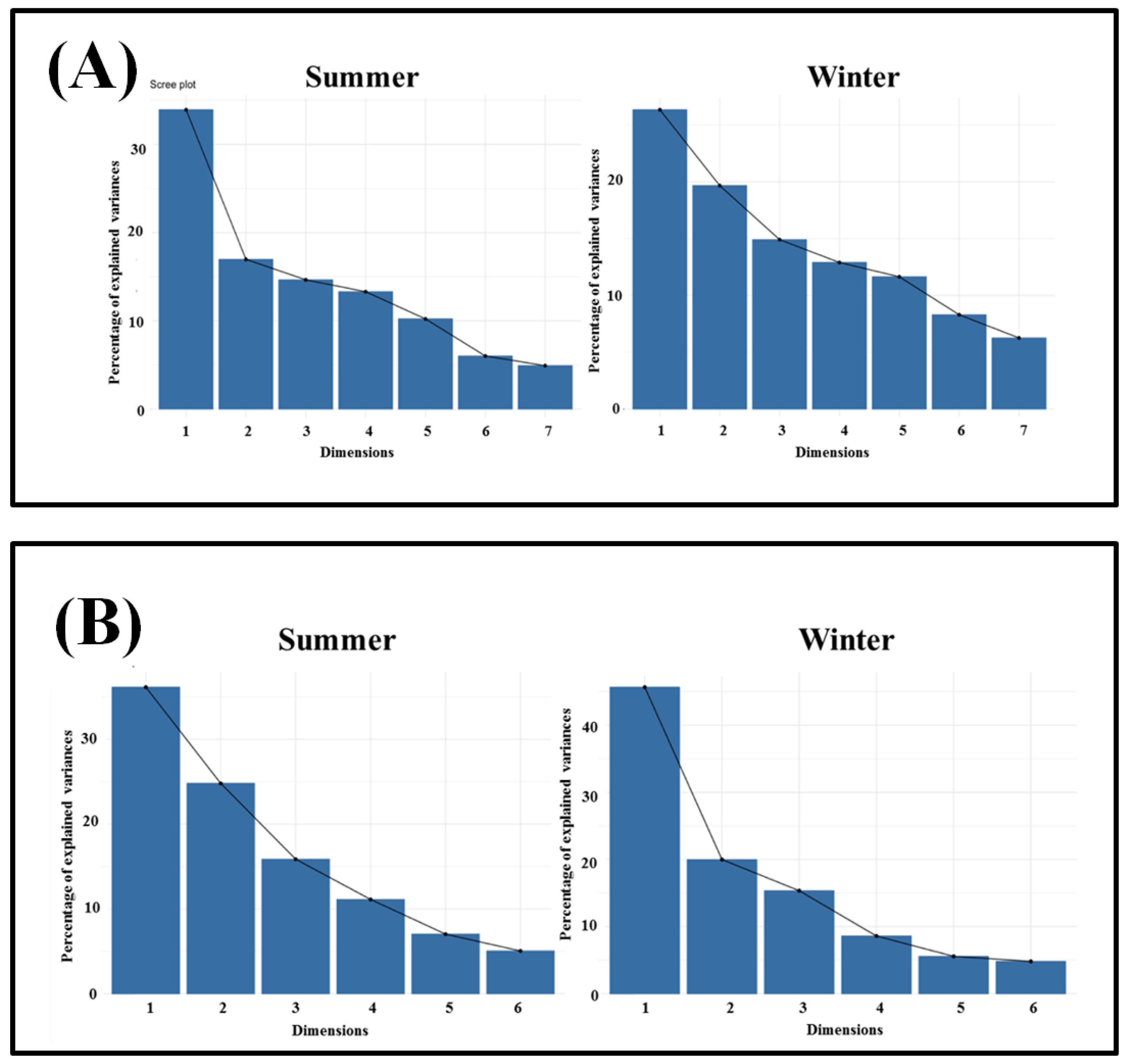
At this stage we performed PCA on both datasets, meteorological and air quality, to investigate whether any variable can explain most of our own dataset. The PCA results for the 7 selected meteorological data are presented in Figure 3 panel A for the summer and winter seasons, separately. The scree plot shows the presence of a principal component which dominates the data during the summer seasons. This variable explains $34\%$ of the total variance of the data.

An analogous analysis was performed for air quality, see Figure 3B. The first PC of the air quality dataset explains $36\%$ and $45.5\%$ for the summer and winter seasons, respectively.

In both cases, to account for at least $90\%$ of the variance, at least the first 3 PCs have to be considered. Since the weights of all variables in the first 3 PCs are not negligible, we conclude that there is no significant benefit in excluding any variable for further analyses.

3.2. Insights from Linear Models

We explored the existence of a linear relationship between meteorological and air quality data. To this aim, we firstly evaluated the pairwise Pearson’s correlation between meteorological and air quality features; the results are shown in

Table 3. Correlation coefficients between the 6 air quality variables and the 7 meteorological variables for both summer (above) and winter (below) period.

SUMMER
Correlation coefficient	T.max	UMR	Prec	WS	WD.	RAD	. Press.Atm.
$N{O}_2$	−0.16	0.04	0.02	−0.27	−0.05	−0.19	−0.00
$CO$	−0.17	0.05	0.00	−0.22	−0.04	−0.13	0.04
$Benzene$	−0.08	0.09	0.01	−0.22	−0.03	−0.08	0.08
$S{O}_2$	0.22	−0.09	−0.02	0.04	0.01	0.15	0.03
$P{M}_{10}$	0.28	−0.14	−0.05	−0.07	−0.04	0.01	0.08
$P{M}_{2.5}$	0.27	−0.07	−0.03	−0.19	−0.06	0.03	0.28
WINTER
Correlation coefficient	T.max	UMR	Prec	WS	WD.	RAD	. Press.Atm.
$N{O}_2$	−0.14	0.09	−0.04	−0.39	0.01	−0.23	0.08
$CO$	−0.25	0.04	−0.06	−0.32	0.03	−0.16	0.14
$Benzene$	−0.18	0.06	−0.06	−0.32	0.06	−0.14	0.18
$S{O}_2$	0.00	−0.06	0.01	−0.01	0.01	0.08	0.01
$P{M}_{10}$	0.09	0.03	−0.06	−0.15	0.02	0.03	0.24
$P{M}_{2.5}$	−0.13	−0.02	−0.08	−0.32	0.08	0.03	0.44

. Correlations were less than moderate, the highest value being 0.44. Accordingly, for both seasons, no linear relationship was identified between any single meteorological and air quality variable.

We also used a linear model to test for the presence of multivariate relationships between meteorological features, used as independent variables, and air quality features, each used as the dependent variable in 6 different models.

In

Table 4. Correlation coefficients for all air quality features for both the summer and winter seasons for the linear model.

Linear Model
Correlation Coefficient	${\mathit{NO}}_{\mathbf{2}}$	$\mathit{CO}$	$\mathit{Benzene}$	${\mathit{SO}}_{\mathbf{2}}$	${\mathit{PM}}_{\mathbf{10}}$	${\mathit{PM}}_{\mathbf{2}.\mathbf{5}}$
SUMMER	0.32	0.27	0.23	0.24	0.34	0.44
WINTER	0.41	0.37	0.36	0.10	0.30	0.50

we report, for each air quality variable, the correlation value between the predicted values from the linear model and the measured values from monitoring station. The whole dataset was used for training and validation. Even in this case, we observe a poor relationship between the meteorological conditions and air quality.

A poor correlation is obtained for all air quality features. In terms of RMSE, the worst performance is obtained by $N{O}_2$ with $\mathrm{RMSE}\approx 0.6$, while for the other pollutants, we obtained on average $\mathrm{RMSE}\approx 0.3$. These findings suggest that linear models cannot model the relationship between meteorological conditions and pollution, if any.

Finally, we investigated the existence of a linear relationship using CCA. Combining 6 air quality and 7 meteorological features, we obtained 6 canonical components. They are the 6 most correlated pairs $(x,y)$ with first component x, a linear combination of air quality features, and with second component y, a linear combination of meteorological features. The results are presented in

Table 5. Correlation coefficients for the 6 pairs of canonical components for the summer and winter seasons.

Canonical Component Analysis
	CC-1	CC-2	CC-3	CC-4	CC-5	CC-6
SUMMER	0.47	0.37	0.25	0.11	0.05	0.03
WINTER	0.57	0.38	0.29	0.09	0.04	0.03

. These results show how the best linear correlation value is $0.47$ during summer and $0.57$ during winter. Both results indicate that, even if we globally consider the meteorological and the air quality data, there is a non-linear relationship between the two datasets.

3.3. Insights from Non-Linear Models

We explored the existence of a non-linear relationship between meteorological conditions and pollution by means of a machine learning approach, namely RF regression. For each of the 6 air quality features, we built a specific RF model. It is worth noting that, as we used RF for modeling purposes, in this case, the whole dataset was used both for training and validation. Of course, we are aware that such a procedure yields a biased estimate of the generalization accuracy; nevertheless, this aspect lies far from the scope of this study. Interestingly, as the dataset dimensions far exceed the number of features exploited by the model, the overfitting issue should be limited. Results are summarized in

Table 6. Correlation coefficients for all air quality features for both the summer and winter seasons for the non-linear models.

Random Forest
Correlation Coefficient	${\mathit{NO}}_{\mathbf{2}}$	$\mathit{CO}$	$\mathit{Benzene}$	${\mathit{SO}}_{\mathbf{2}}$	${\mathit{PM}}_{\mathbf{10}}$	${\mathit{PM}}_{\mathbf{2}.\mathbf{5}}$
SUMMER	0.93	0.94	0.93	0.94	0.95	0.94
WINTER	0.92	0.92	0.92	0.93	0.94	0.93

.

From the comparison among Table 5 and Table 6, it is evident that the RF model outperforms the linear models.

3.4. Air Quality Data Predictions

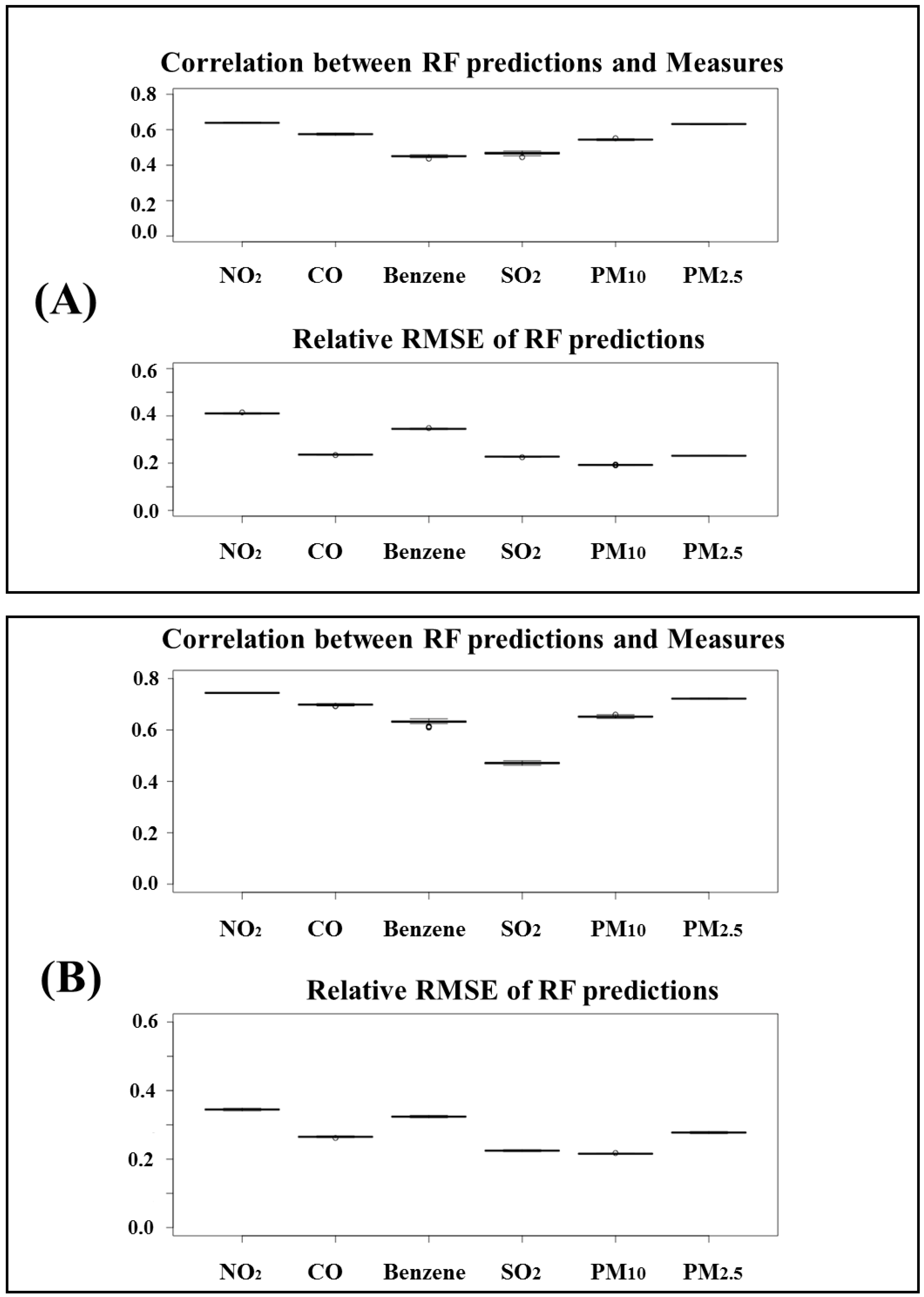
The result obtained with RF trained on the whole dataset suggests the possibility to use a RF model for prediction purposes. We explored the possibility of modeling the air quality using meteorological predictors. In this case, we adopted a 5-fold cross-validation framework repeated 100 times. In order not to alter the configuration of the RF model investigated previously, we performed the analysis separately for the summer and winter periods. Figure 4 shows both the summer and winter results. As expected, we observe a performance deterioration with respect to Table 6. Except for $S{O}_2$ and benzene, correlations exceed $0.5$. In terms of $\mathrm{RMSE}$, performance for all pollutants remains stable, except for $N{O}_2$. Interestingly, despite the cross validation, the variance of the performance measured in terms of the interquartile range of the boxplots is extremely small, suggesting particularly robust results. We reported additional figures and tables with the results of our analysis in Supplementary Materials section.

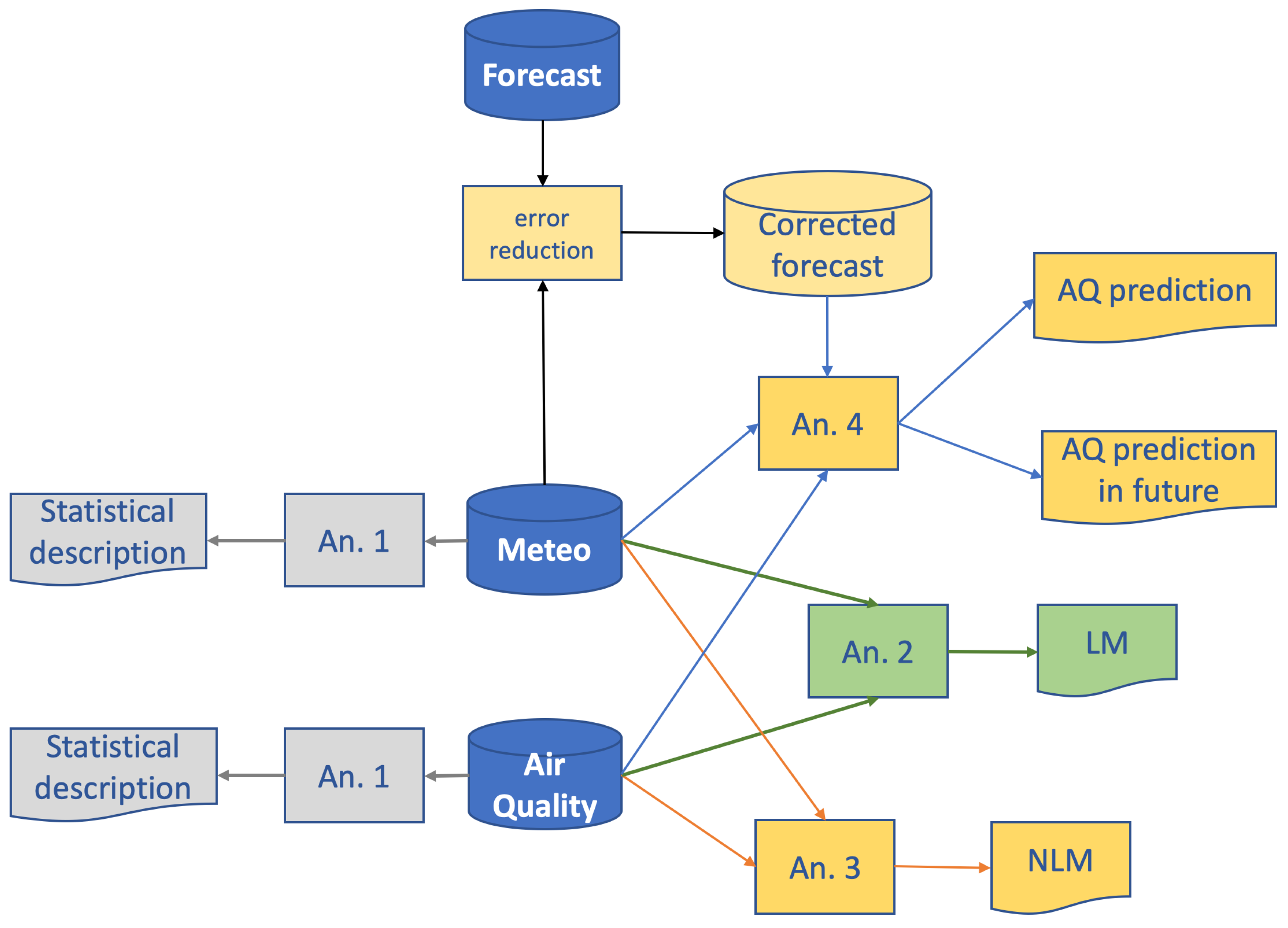
The previous results demonstrated how meteorological conditions at time t can be suitably used to predict the air quality at the same time t. Here, we address the problem of forecasting air quality at future times $t+h$. In particular, using the numerical weather prediction model WRF, we investigated three distinct cases: $h=24,48,72$ h, 1, 2, and 3 days in advance, respectively. Furthermore, we compared results obtained using data with spatial resolution d01 (16 km) and d02 (4 km). Finally, as the ground station has its own geographical coordinates which do not coincide with a node of the grid, we used the GrADS software to allow the comparison and applied post-processing techniques to reduce the forecast error for those measures acquired on ground: 2 m temperature, 10 m temperature, 10 m wind direction and speed, and 2 m relative humidity. We assessed the performance in terms of MSE and Pearson’s correlation.

The forecast error reduction approach basically consists in training a specific RF model on a period of 30 days prior to the day of interest in order to predict the WRF bias on the estimation of the weather variables. This approach proved effective in reducing the average forecast error to the point of making it close to zero. In the case of the wind speed of 10 m, in addition to reducing the systematic error, this approach also reduced the error globally.

This error reduction occurred for all the considered variables, except for the 10 m wind direction (for the temperature at 2 m, no significant improvement was observed because the forecast was already excellent). However, for the 10 m wind direction, this approach effectively reduced the direction accuracy (DACC). For a detailed description of the forecast error reduction in the predicted WRF variables, see the Supporting Material section.

Once the WRF prediction mean error was reduced, a new RF model was trained for each of the air quality variables, in the same way as in the previous analysis, with the difference that the measured weather values were replaced by the WRF predicted and corrected weather values. Since the WRF model was used to obtain forecasts with 1, 2 and 3 days in advance on two spatial domains with resolutions of 16 and 4 km, respectively, the same number of air quality variable predictions are available.

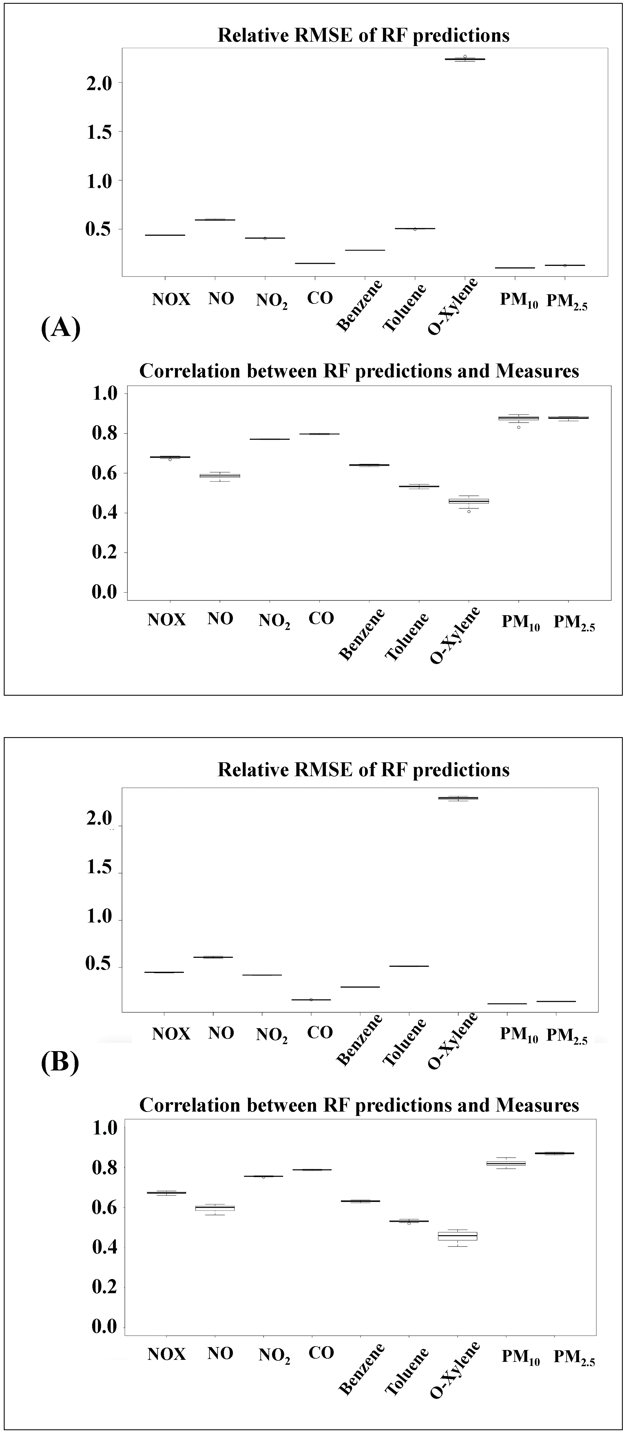
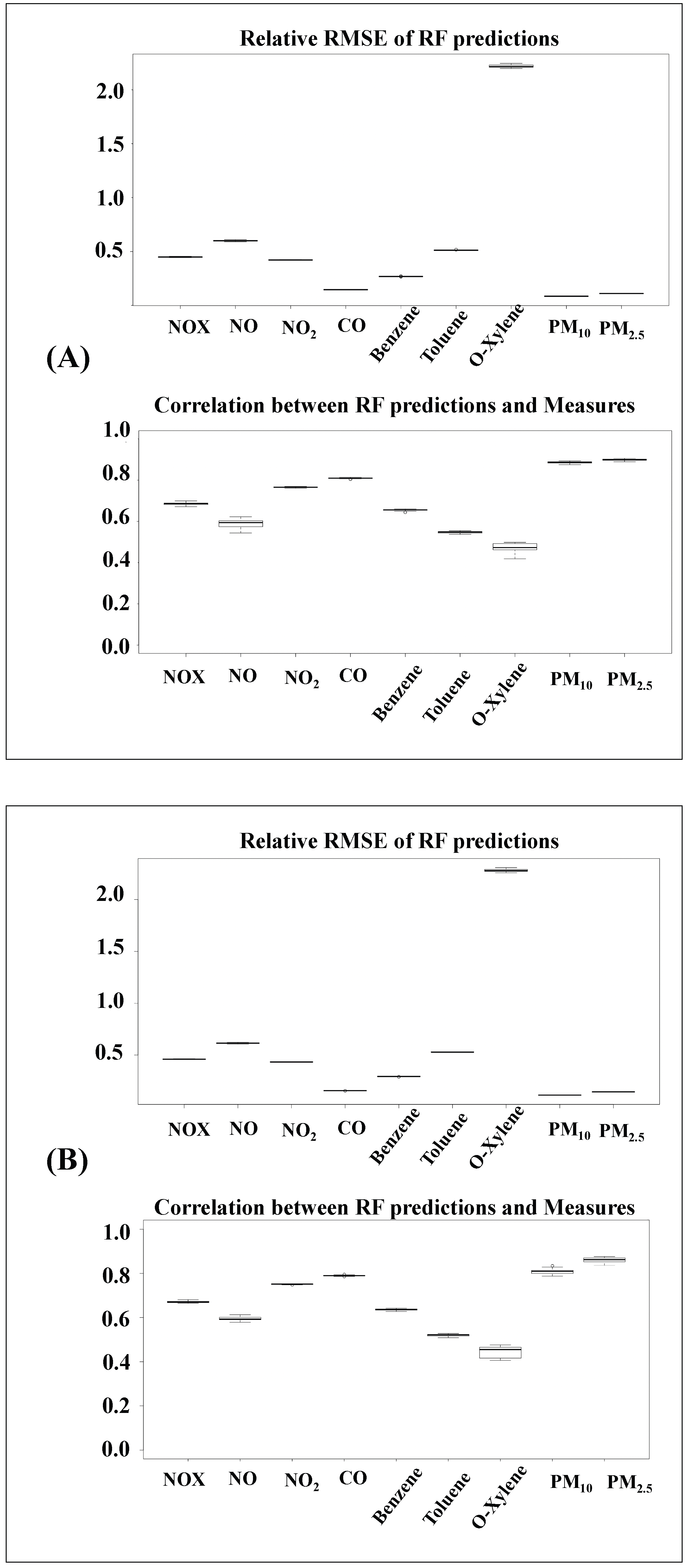
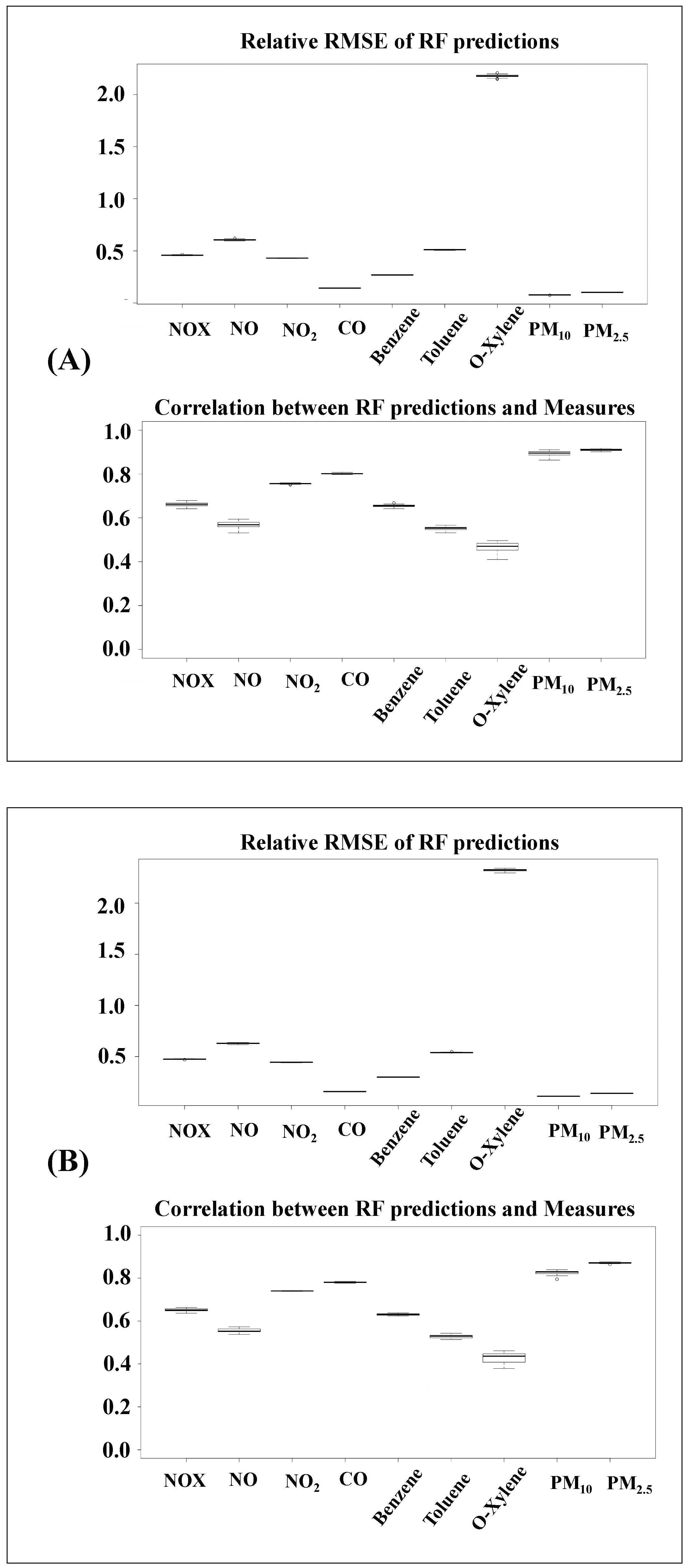
In panel A of Figure 5, Figure 6 and Figure 7, we show the performance of each of the 9 models in terms of relative RMSE and correlation coefficient on the lowest resolution domain d01 using 1-, 2- or 3-day forecasts, respectively.

In panel B of Figure 5, Figure 6 and Figure 7, the performance for each of the 9 models in terms of relative RMSE and correlation coefficient on the higher resolution domain d02 using 1-, 2- or 3-day forecasts, respectively, are shown.

The results show that regardless of the spatial domain and the type of forecast, the RF models for the prediction of air quality achieve good performance in terms of the correlation coefficient (higher than $0.7$) for $N{O}_2$, $CO$, $P{M}_{10}$, and $P{M}_{2.5}$. If for $CO$, $P{M}_{10}$, and $P{M}_{2.5}$, the relative RMSE is excellent, as it is lower than $0.2$, and for $N{O}_2$, despite the good correlation between the predicted and measured values, the relative RMSE is $0.4$. In the Supporting Material section, we reported scatter plots and time series for the four air quality variables showed good performance. Given the length of the analyzed time window, for the time series, we considered only the first four months of the considered period.

4. Conclusions

In this work, we analyzed the peculiar case of the Southern Italian province of Lecce in the Apulia region. This province has the highest tumor rate in the region despite heavy industries being substantially absent. We hypothesize here that meteorological conditions affect the air quality of this province. Using machine learning, we combine ground and forecast meteorological factors with air quality data to investigate possible interactions between them. The study, through the use of typical machine learning techniques, confirms the existence of a relationship between meteorological data and air quality data and shows that this relationship is certainly non-linear.

Using this relationship, it is possible to both predict current air quality data using the current measured meteorological data and predict future values of air quality variables using weather forecasts.

The relationship between meteorological data and air quality data is not univocal but is site-specific and also dependent on seasonality and therefore cannot be generalized. For this reason, although numerous studies have already been conducted in this regard, each referring to a specific location, it is necessary to repeat the analyses for each new site of interest.

Of course, our study was affected by the typical limitations of ecological studies; however, it is worth noting that our goal was not to demonstrate a causal relationship. Our findings reveal a significant association between meteorological conditions and the concentrations of $P{M}_{10}$, $P{M}_{2.5}$, $NO$₂ and $CO$. In a future study, it might be of interest to analyze whether such an association could explain the anomalous tumor rate in the studied region, which does not have any heavy industries. In fact, high concentrations of pollutants can result from specific meteorological conditions that, for instance, influence the depth of the planetary boundary layer, and cause air stagnation, the long-range transport of pollutants, or other phenomena.

References

1. Lionetto, M.G.; Guascito, M.R.; Caricato, R.; Giordano, M.E.; De Bartolomeo, A.R.; Romano, M.P.; Conte, M.; Dinoi, A.; Contini, D. Correlation of oxidative potential with ecotoxicological and cytotoxicological potential of PM10 at an urban background site in Italy. Atmosphere 2019, 10, 733. [Google Scholar] [CrossRef] [Green Version]
2. Pope III, C.A.; Dockery, D.W. Health effects of fine particulate air pollution: Lines that connect. J. Air Waste Manag. Assoc. 2006, 56, 709–742. [Google Scholar] [CrossRef] [PubMed]
3. Gualtieri, M.; Longhin, E.; Mattioli, M.; Mantecca, P.; Tinaglia, V.; Mangano, E.; Proverbio, M.C.; Bestetti, G.; Camatini, M.; Battaglia, C. Gene expression profiling of A549 cells exposed to Milan PM2.5. Toxicol. Lett. 2012, 209, 136–145. [Google Scholar] [CrossRef] [PubMed]
4. Gauderman, W.J.; Urman, R.; Avol, E.; Berhane, K.; McConnell, R.; Rappaport, E.; Chang, R.; Lurmann, F.; Gilliland, F. Association of improved air quality with lung development in children. N. Engl. J. Med. 2015, 372, 905–913. [Google Scholar] [CrossRef] [PubMed] [Green Version]
5. Velali, E.; Papachristou, E.; Pantazaki, A.; Choli-Papadopoulou, T.; Planou, S.; Kouras, A.; Manoli, E.; Besis, A.; Voutsa, D.; Samara, C. Redox activity and in vitro bioactivity of the water-soluble fraction of urban particulate matter in relation to particle size and chemical composition. Environ. Pollut. 2016, 208, 774–786. [Google Scholar] [CrossRef]
6. Perrone, M.G.; Gualtieri, M.; Ferrero, L.; Porto, C.L.; Udisti, R.; Bolzacchini, E.; Camatini, M. Seasonal variations in chemical composition and in vitro biological effects of fine PM from Milan. Chemosphere 2010, 78, 1368–1377. [Google Scholar] [CrossRef]
7. Happo, M.; Markkanen, A.; Markkanen, P.; Jalava, P.; Kuuspalo, K.; Leskinen, A.; Sippula, O.; Lehtinen, K.; Jokiniemi, J.; Hirvonen, M.R. Seasonal variation in the toxicological properties of size-segregated indoor and outdoor air particulate matter. Toxicol. Vitr. 2013, 27, 1550–1561. [Google Scholar] [CrossRef]
8. Jia, Y.Y.; Wang, Q.; Liu, T. Toxicity research of PM2.5 compositions in vitro. Int. J. Environ. Res. Public Health 2017, 14, 232. [Google Scholar] [CrossRef] [Green Version]
9. Li, N.; Sioutas, C.; Cho, A.; Schmitz, D.; Misra, C.; Sempf, J.; Wang, M.; Oberley, T.; Froines, J.; Nel, A. Ultrafine particulate pollutants induce oxidative stress and mitochondrial damage. Environ. Health Perspect. 2003, 111, 455–460. [Google Scholar] [CrossRef] [Green Version]
10. Delfino, R.J.; Staimer, N.; Tjoa, T.; Gillen, D.L.; Schauer, J.J.; Shafer, M.M. Airway inflammation and oxidative potential of air pollutant particles in a pediatric asthma panel. J. Expo. Sci. Environ. Epidemiol. 2013, 23, 466–473. [Google Scholar] [CrossRef]
11. Michael, S.; Montag, M.; Dott, W. Pro-inflammatory effects and oxidative stress in lung macrophages and epithelial cells induced by ambient particulate matter. Environ. Pollut. 2013, 183, 19–29. [Google Scholar] [CrossRef]
12. Donaldson, K.; Stone, V.; Borm, P.J.; Jimenez, L.A.; Gilmour, P.S.; Schins, R.P.; Knaapen, A.M.; Rahman, I.; Faux, S.P.; Brown, D.M.; et al. Oxidative stress and calcium signaling in the adverse effects of environmental particles (PM10). Free Radic. Biol. Med. 2003, 34, 1369–1382. [Google Scholar] [CrossRef]
13. Brugha, R.; Grigg, J. Urban air pollution and respiratory infections. Paediatr. Respir. Rev. 2014, 15, 194–199. [Google Scholar] [CrossRef]
14. Kleine Deters, J.; Zalakeviciute, R.; Gonzalez, M.; Rybarczyk, Y. Modeling PM2.5 urban pollution using machine learning and selected meteorological parameters. J. Electr. Comput. Eng. 2017, 2017, 5106045. [Google Scholar] [CrossRef] [Green Version]
15. World Health Organization. Air Pollution Levels Rising in Many of the World’s Poorest Cities. 2016. Available online: https://www.who.int/news/item/12-05-2016-air-pollution-levels-rising-in-many-of-the-world-s-poorest-cities (accessed on 10 October 2022).
16. Lelieveld, J.; Evans, J.S.; Fnais, M.; Giannadaki, D.; Pozzer, A. The contribution of outdoor air pollution sources to premature mortality on a global scale. Nature 2015, 525, 367–371. [Google Scholar] [CrossRef]
17. Xing, Y.F.; Xu, Y.H.; Shi, M.H.; Lian, Y.X. The impact of PM2.5 on the human respiratory system. J. Thorac. Dis. 2016, 8, E69. [Google Scholar]
18. Carugno, M.; Dentali, F.; Mathieu, G.; Fontanella, A.; Mariani, J.; Bordini, L.; Milani, G.P.; Consonni, D.; Bonzini, M.; Bollati, V.; et al. PM10 exposure is associated with increased hospitalizations for respiratory syncytial virus bronchiolitis among infants in Lombardy, Italy. Environ. Res. 2018, 166, 452–457. [Google Scholar] [CrossRef]
19. Conticini, E.; Frediani, B.; Caro, D. Can atmospheric pollution be considered a co-factor in extremely high level of SARS-CoV-2 lethality in Northern Italy? Environ. Pollut. 2020, 261, 114465. [Google Scholar] [CrossRef]
20. Sciomer, S.; Moscucci, F.; Magrì, D.; Badagliacca, R.; Piccirillo, G.; Agostoni, P. SARS-CoV-2 spread in Northern Italy: What about the pollution role? Environ. Monit. Assess. 2020, 192, 325. [Google Scholar] [CrossRef]
21. Setti, L.; Passarini, F.; De Gennaro, G.; Barbieri, P.; Pallavicini, A.; Ruscio, M.; Piscitelli, P.; Colao, A.; Miani, A. Searching for SARS-COV-2 on Particulate Matter: A Possible Early Indicator of COVID-19 Epidemic Recurrence. Int. J. Environ. Res. Public Health. 2020, 17, 2986. [Google Scholar] [CrossRef]
22. Gatti, R.C.; Velichevskaya, A.; Tateo, A.; Amoroso, N.; Monaco, A. Machine learning reveals that prolonged exposure to air pollution is associated with SARS-CoV-2 mortality and infectivity in Italy. Environ. Pollut. 2020, 267, 115471. [Google Scholar] [CrossRef] [PubMed]
23. Ciencewicki, J.; Jaspers, I. Air pollution and respiratory viral infection. Inhal. Toxicol. 2007, 19, 1135–1146. [Google Scholar] [CrossRef] [PubMed]
24. Wong, C.M.; Thach, T.Q.; Chau, P.; Chan, E.; Chung, R.Y.n.; Ou, C.Q.; Yang, L.; Peiris, J.; Thomas, G.N.; Lam, T.H.; et al. Part 4. Interaction between Air Pollution and Respiratory Viruses: Time-Series Study of Daily Mortality and Hospital Admissions in Hong Kong; Research Report; Health Effects Institute: Boston, MA, USA, 2010; pp. 283–362. [Google Scholar]
25. Nenna, R.; Evangelisti, M.; Frassanito, A.; Scagnolari, C.; Pierangeli, A.; Antonelli, G.; Nicolai, A.; Arima, S.; Moretti, C.; Papoff, P.; et al. Respiratory syncytial virus bronchiolitis, weather conditions and air pollution in an Italian urban area: An observational study. Environ. Res. 2017, 158, 188–193. [Google Scholar] [CrossRef] [PubMed]
26. Ramsey, N.R.; Klein, P.M.; Moore, B. The impact of meteorological parameters on urban air quality. Atmos. Environ. 2014, 86, 58–67. [Google Scholar] [CrossRef]
27. Wang, J.; Ogawa, S. Effects of meteorological conditions on PM2.5 concentrations in Nagasaki, Japan. Int. J. Environ. Res. Public Health 2015, 12, 9089–9101. [Google Scholar] [CrossRef]
28. Zhang, F.; Cheng, H.r.; Wang, Z.w.; Lv, X.p.; Zhu, Z.m.; Zhang, G.; Wang, X.m. Fine particles (PM2.5) at a CAWNET background site in Central China: Chemical compositions, seasonal variations and regional pollution events. Atmos. Environ. 2014, 86, 193–202. [Google Scholar] [CrossRef]
29. Li, Y.; Chen, Q.; Zhao, H.; Wang, L.; Tao, R. Variations in PM10, PM2.5 and PM1.0 in an urban area of the Sichuan Basin and their relation to meteorological factors. Atmosphere 2015, 6, 150–163. [Google Scholar] [CrossRef] [Green Version]
30. Lombardi, A.; Diacono, D.; Amoroso, N.; Monaco, A.; Tavares, J.M.R.; Bellotti, R.; Tangaro, S. Explainable deep learning for personalized age prediction with brain morphology. Front. Neurosci. 2021, 15, 578. [Google Scholar] [CrossRef]
31. Amoroso, N.; Pomarico, D.; Fanizzi, A.; Didonna, V.; Giotta, F.; La Forgia, D.; Latorre, A.; Monaco, A.; Pantaleo, E.; Petruzzellis, N.; et al. A roadmap towards breast cancer therapies supported by explainable artificial intelligence. Appl. Sci. 2021, 11, 4881. [Google Scholar] [CrossRef]
32. Tateo, A.; Miglietta, M.M.; Fedele, F.; Menegotto, M.; Monaco, A.; Bellotti, R. Ensemble using different Planetary Boundary Layer schemes in WRF model for wind speed and direction prediction over Apulia region. Adv. Sci. Res. 2017, 14, 95–102. [Google Scholar] [CrossRef] [Green Version]
33. Fedele, F.; Miglietta, M.M.; Perrone, M.R.; Burlizzi, P.; Bellotti, R.; Conte, D.; Carducci, A.G.C. Numerical simulations with the WRF model of water vapour vertical profiles: A comparison with LIDAR and radiosounding measurements. Atmos. Res. 2015, 166, 110–119. [Google Scholar] [CrossRef]
34. Berman, F.; Chien, A.; Cooper, K.; Dongarra, J.; Foster, I.; Gannon, D.; Johnsson, L.; Kennedy, K.; Kesselman, C.; Mellor-Crumme, J.; et al. The GrADS project: Software support for high-level grid application development. Int. J. High Perform. Comput. Appl. 2001, 15, 327–344. [Google Scholar] [CrossRef]
35. Abdi, H.; Williams, L.J. Principal component analysis. Wiley Interdiscip. Rev. Comput. Stat. 2010, 2, 433–459. [Google Scholar] [CrossRef]
36. Meuzelaar, H.; Statheropoulos, M.; Huai, H.; Yun, Y. Canonical Correlation Analysis of Multisource Fossil Fuel Data. Comput.-Enhanc. Anal. Spectrosc. Peter A. Jurs Plenum Publ. 1992, 111, 185–213. [Google Scholar]
37. Statheropoulos, M.; Vassiliadis, N.; Pappa, A. Principal component and canonical correlation analysis for examining air pollution and meteorological data. Atmos. Environ. 1998, 32, 1087–1095. [Google Scholar] [CrossRef]
38. Breiman, L. Random forests. Mach. Learn. 2001, 45, 5–32. [Google Scholar] [CrossRef] [Green Version]
39. Tateo, A.; Bellotti, R.; Fedele, F.; Guarnieri Calò Carducci, A.; Pollice, A. Post-processing of the Weather Research and Forecasting (WRF) Mesoscale Model by Artificial Neural Networks. In Proceedings of the GRASPA-SIS Biennial Conference, Bari, Italy, 15–16 June 2015. [Google Scholar]
Figure 1. Overall flowchart of the proposed methodology. AQ: air quality; LM: linear model; NLM: non-linear model; An.1: step 1 of the analysis; An.2: step 2 of the analysis; An.3: step 3 of the analysis; An.4: step 4 of the analysis.
Atmosphere 14 00475 g001
Figure 2. Map of Italy with Lecce location (panel A); plant of Lecce, the position of monitoring station (panel B).
Atmosphere 14 00475 g002
Figure 3. Percentage of variance explained by each principal component during summer (left) and winter (right) for the meteorological data (A) and air quality data (B).
Atmosphere 14 00475 g003
Figure 4. Distributions of the correlation (top) and the relative RMSE (bottom) of random forest predictions vs. measured values for each air quality variable, obtained from 100 repeated 5-fold cross-validation procedures, for the summer (A) and winter seasons (B).
Atmosphere 14 00475 g004
Figure 5. Distributions of the relative RMSE (top) and Pearson’s correlation coefficient (bottom) for each RF model using the WRF prediction for the first day (+24) on the lower resolution domain d01 (A) and on the higher resolution domain d02 (B).
Atmosphere 14 00475 g005
Figure 6. Distributions of the relative RMSE (top) and Pearson’s correlation coefficient (bottom) for each RF model using the WRF prediction for the second day (+48) on the lower resolution domain d01 (A) and on the higher resolution domain d02 (B).
Atmosphere 14 00475 g006
Figure 7. Distributions of the relative RMSE (top) and Pearson’s correlation coefficient (bottom) for each RF model using the WRF prediction for the third day (+72) on the lower resolution domain d01 (A) and on the higher resolution domain d02 (B).
Atmosphere 14 00475 g007