
Is There a Formaldehyde Deficit in Emissions Inventories for Southeast Michigan?

 ,
,
Abstract
:1. Introduction
2. Methods
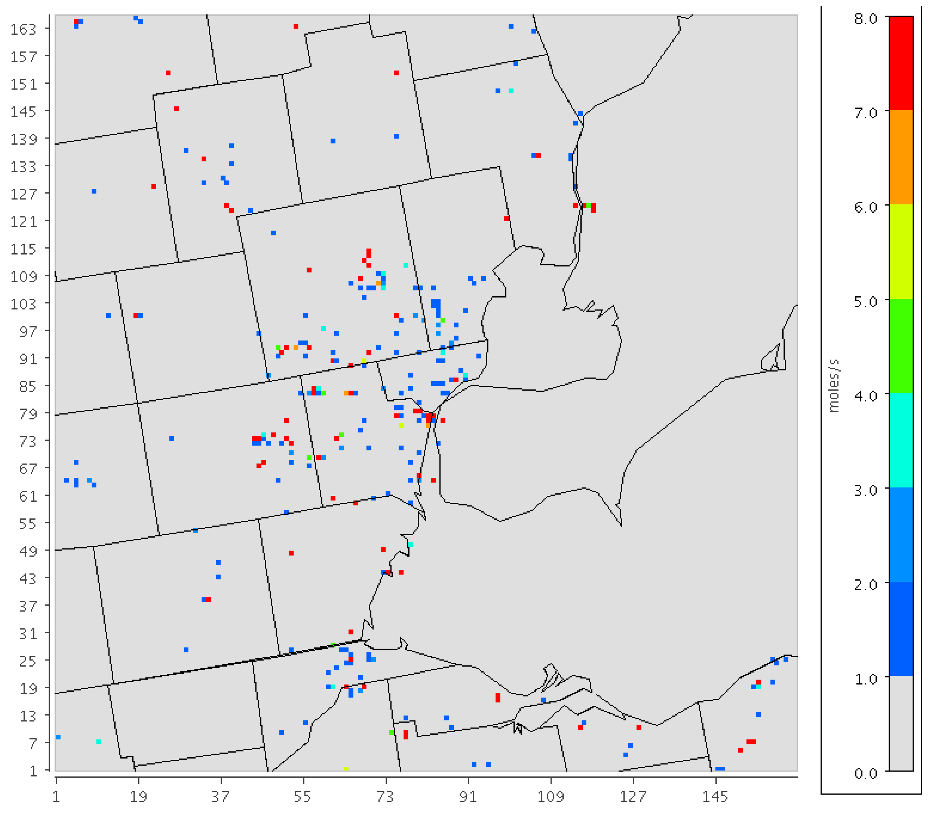
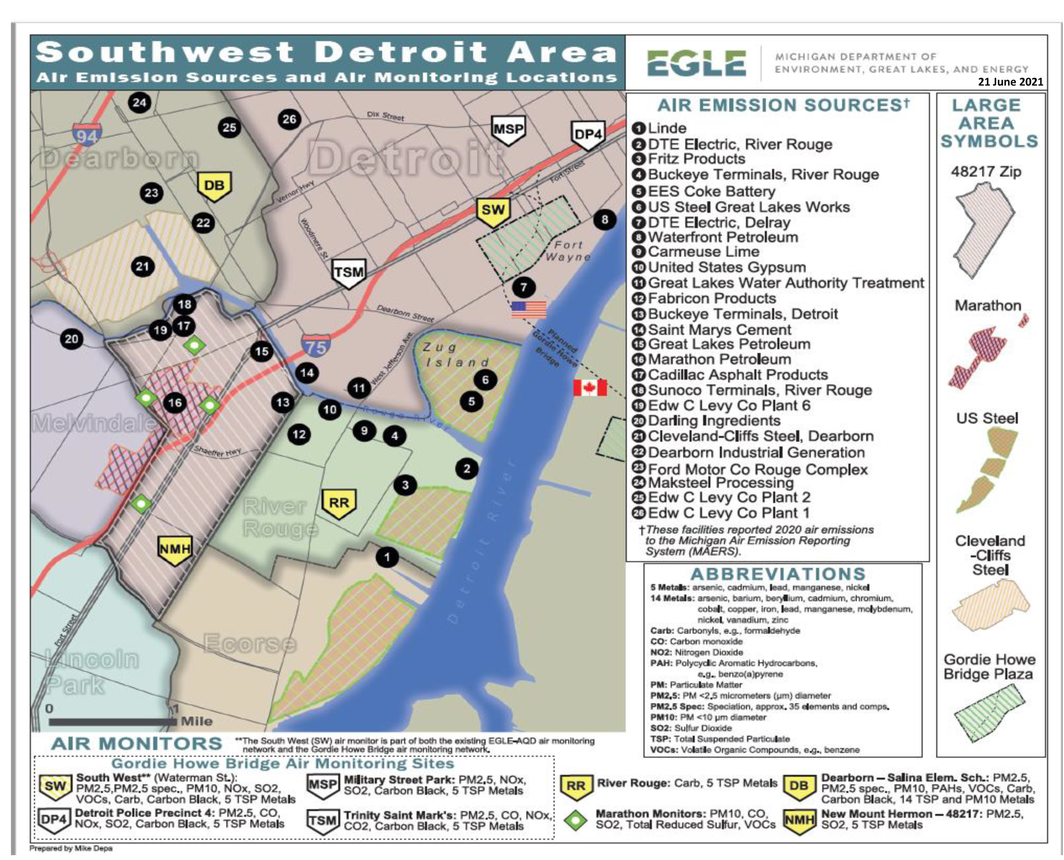
2.1. Formaldehyde Emissions Estimates
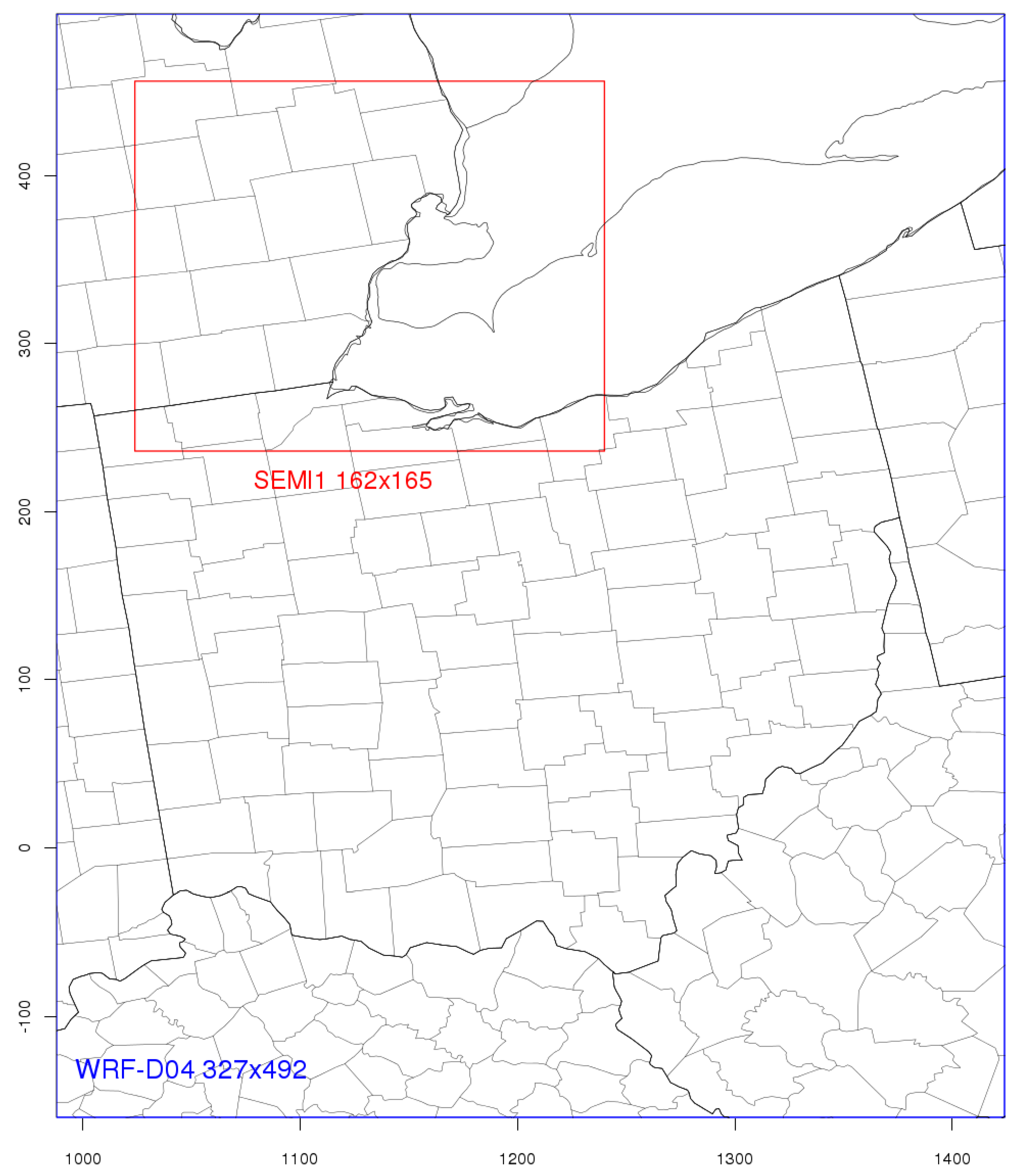
2.2. Modeling Methodology
2.3. Field Measurements
3. Results
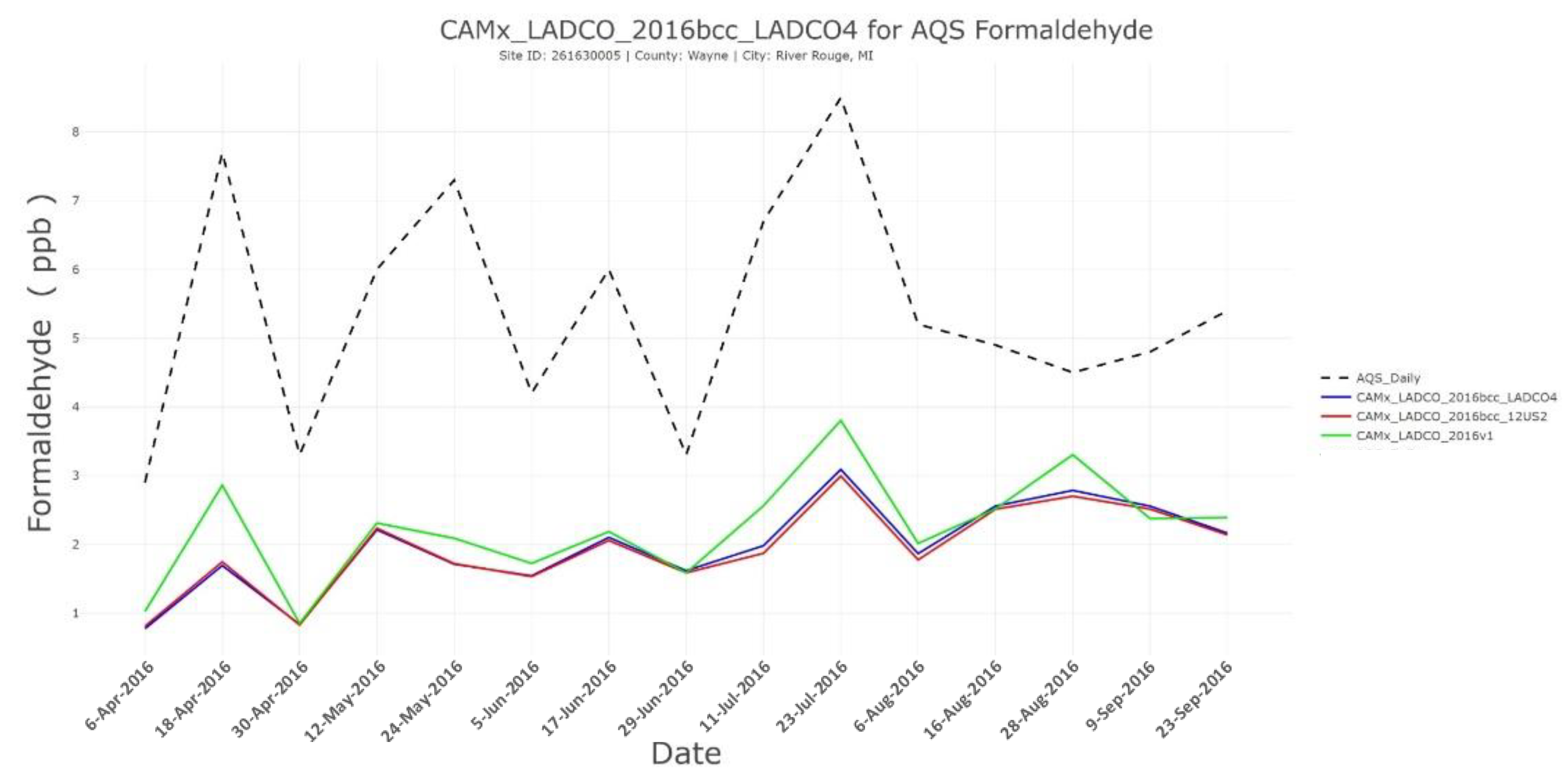
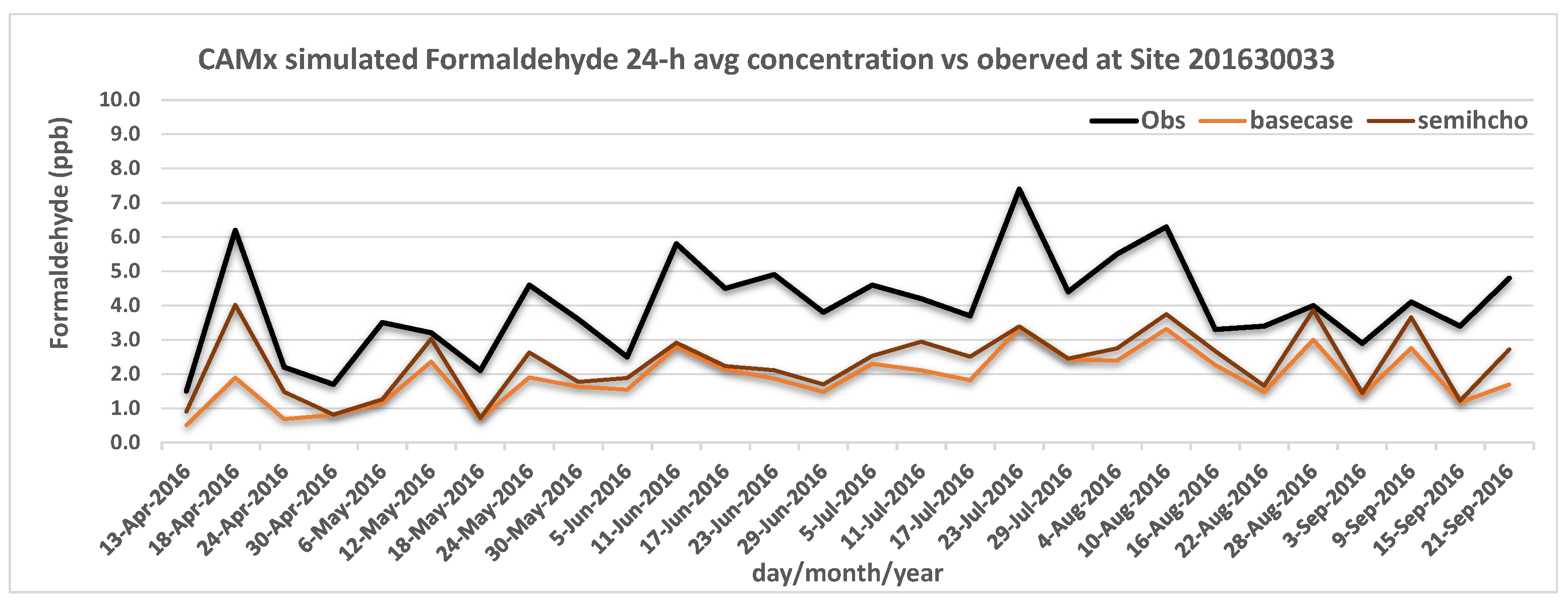
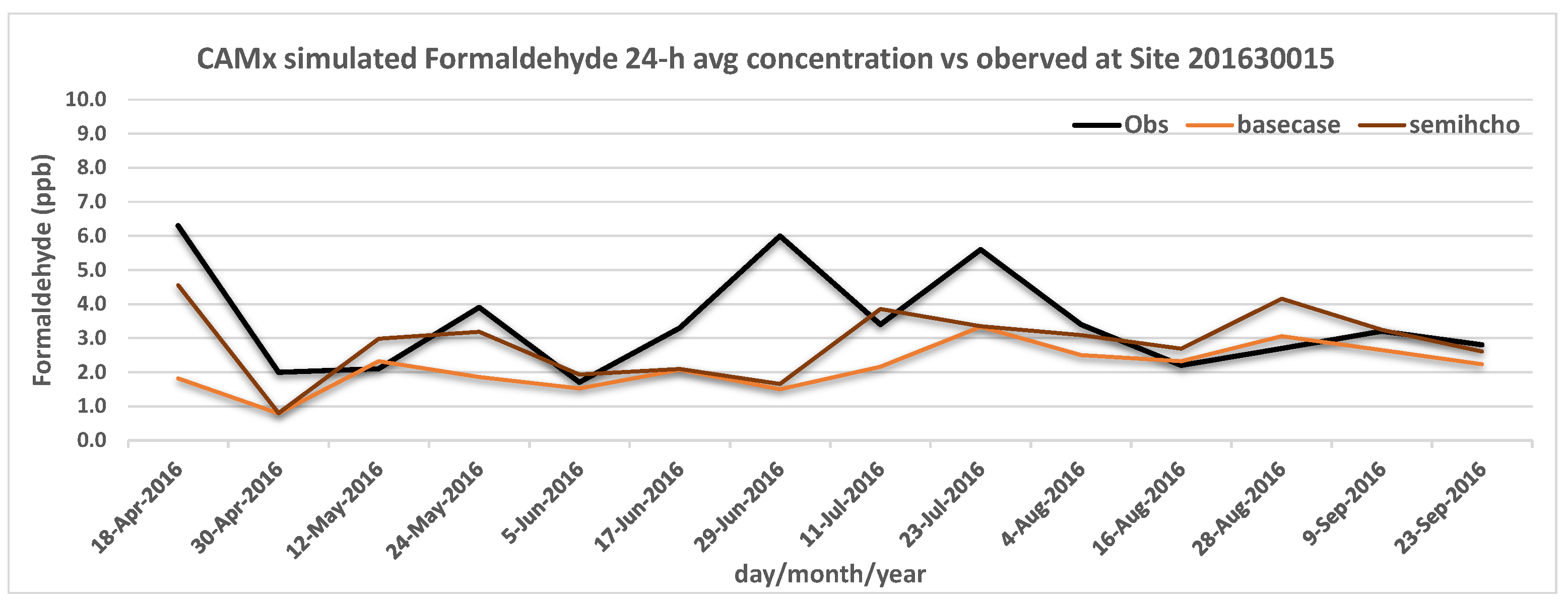
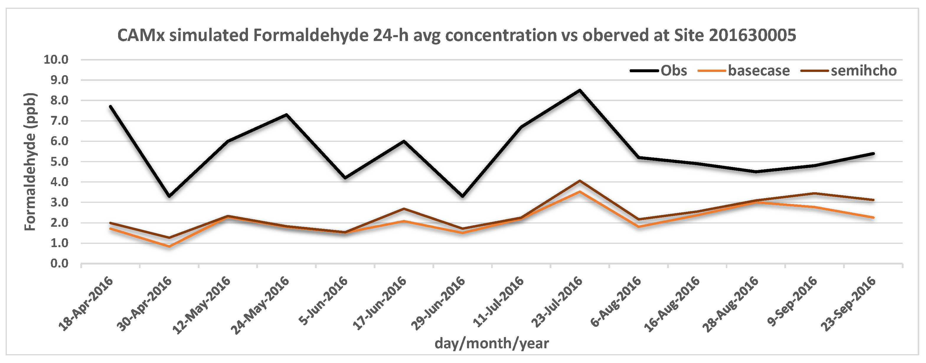
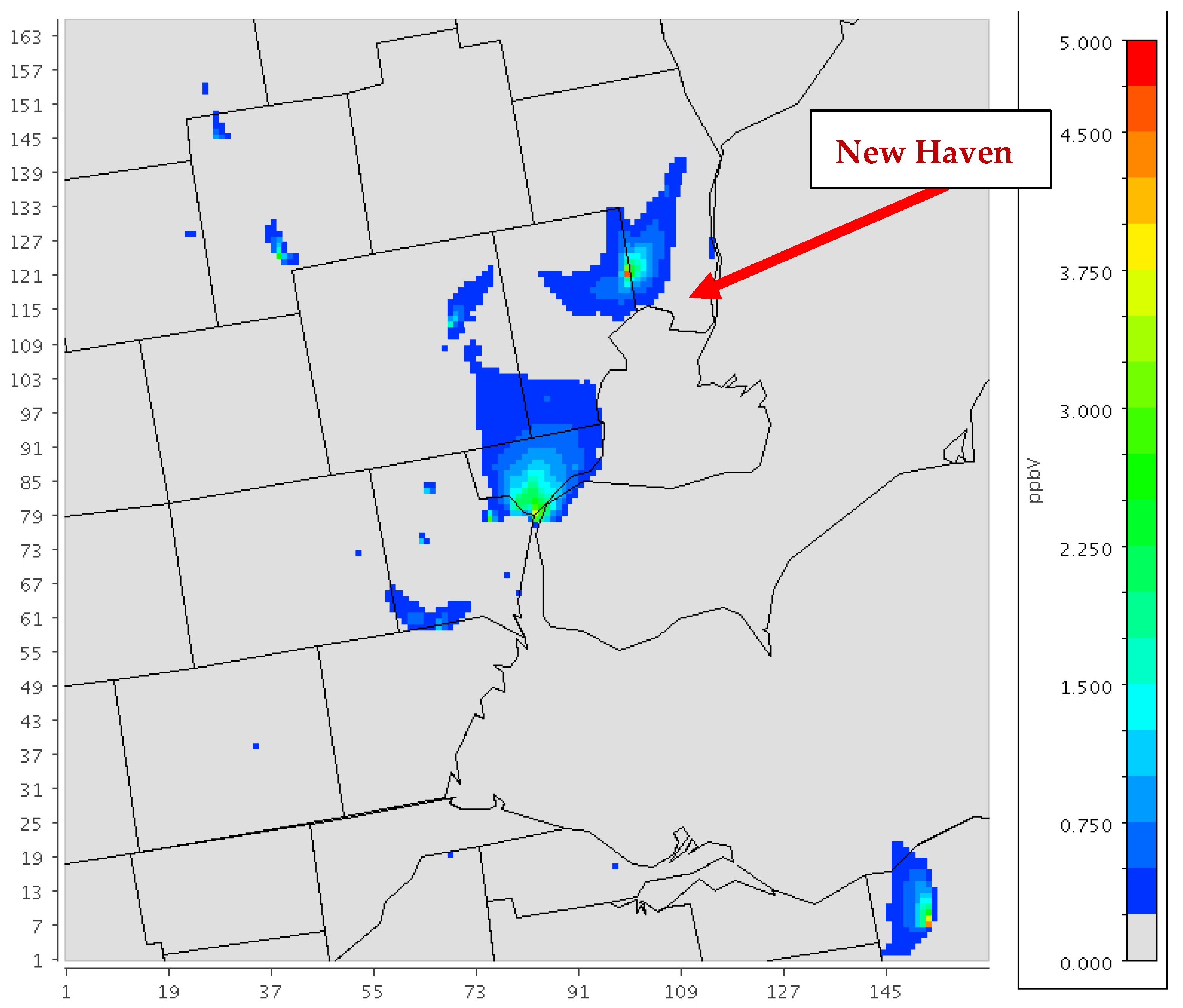
3.1. CAMx Modeling
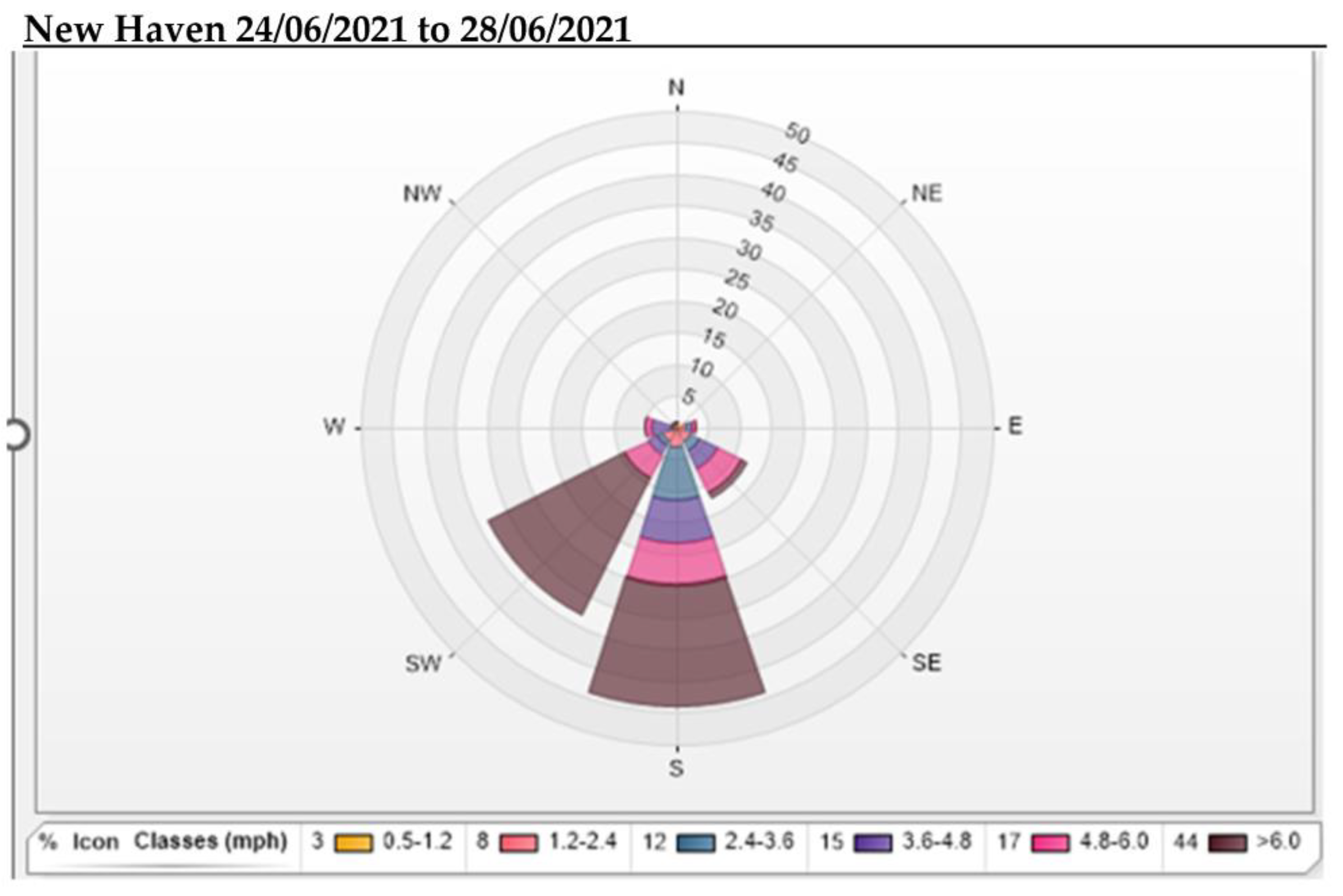
3.2. HCHO Measurements
4. Discussion
5. Summary and Conclusions
- Primary HCHO is significantly underestimated in current emissions inventories due to the under-deployment of contemporary emission measurement techniques.
- Ambient HCHO concentrations near the surface in heavily industrialized urban areas are likely under-predicted by air quality models due to a deficit in primary HCHO, and not merely because existing model chemical mechanisms under-predict secondary HCHO due to biogenic isoprene emissions.
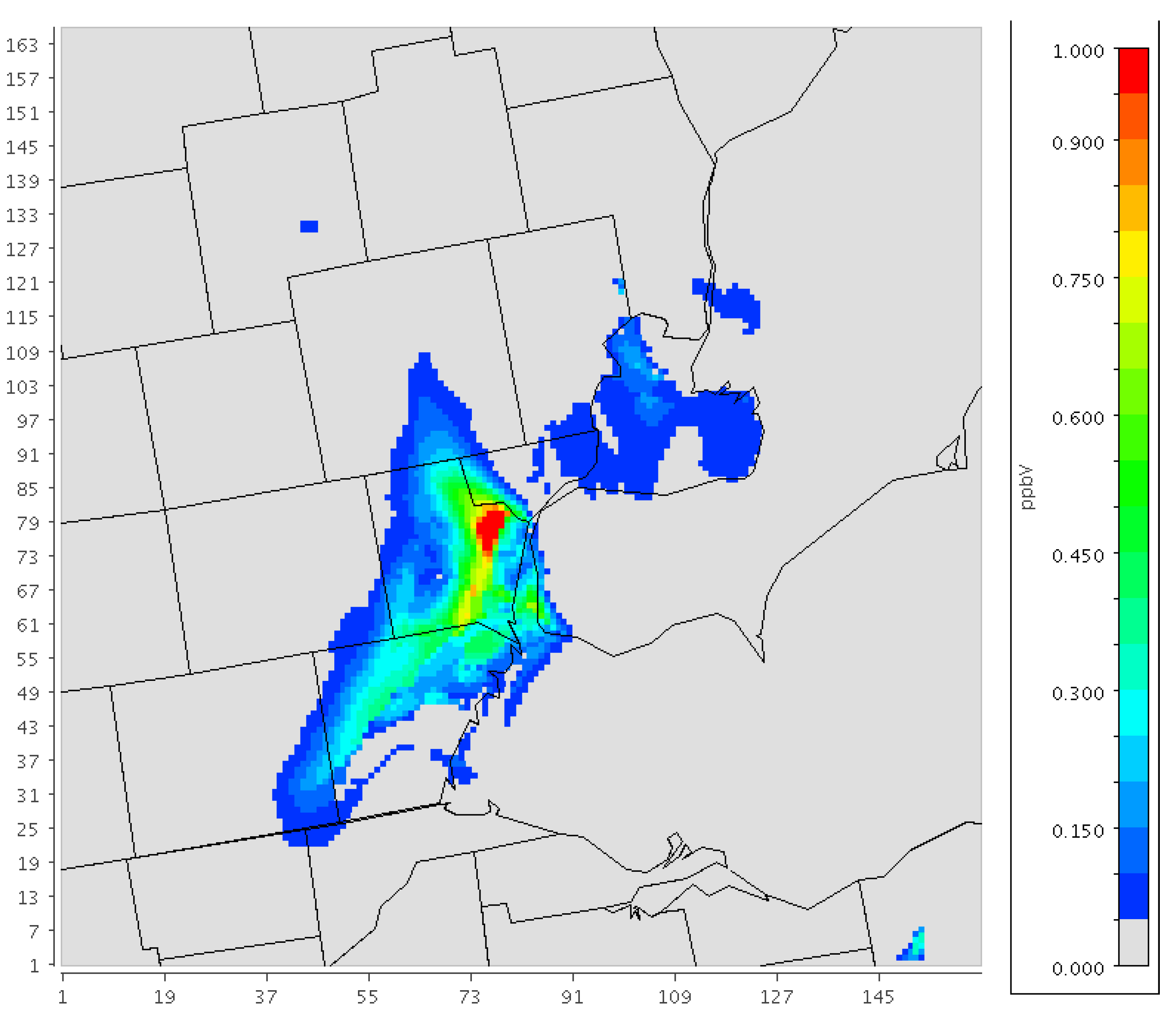
- The MDA8 O3 attributable to missing HCHO emissions can approach or exceed 1 ppb in areas downwind of HCHO emission sources.
- Controlling emissions of HCHO may yield significant human health benefits beyond mitigating human exposure to ambient ozone by reducing toxics exposure, especially in industrial fence line communities.
Author Contributions
Funding
Institutional Review Board Statement
Informed Consent Statement
Data Availability Statement
Conflicts of Interest
References
- Calvert, J.G.; Orlando, J.J.; Stockwell, W.R.; Wallington, T.J. The Mechanisms of Reactions Influencing Atmospheric Ozone; Oxford University Press: New York, NY, USA, 2015. [Google Scholar]
- Mao, J.; Ren, X.; Chen, S.; Brune, W.H.; Chen, Z.; Martinez, M.; Hader, H.; Lefer, B.; Rappenglück, B.; Flynn, J.; et al. Atmospheric oxidation capacity in the summer of Houston 2006: Comparison with summer measurements in other metropolitan studies. Atmos. Environ. 2010, 44, 4107–4115. [Google Scholar] [CrossRef]
- Dovrou, E.; Bates, K.H.; Moch, J.M.; Keutsch, F.N. Catalytic role of formaldehyde in particulate matter formation. Proc. Natl. Acad. Sci. USA 2022, 119, e2113265119. [Google Scholar] [CrossRef]
- U.S. Environmental Protection Agency. Integrated Risk Information System (IRIS) on Formaldehyde; National Center for Environmental Assessment, Office of Research and Development: Washington, DC, USA, 1999.
- U.S. Environmental Protection Agency. IRIS Toxicological Review of Formaldehyde-Inhalation (External Review Draft); EPA/635/R-22/039; U.S. Environmental Protection Agency: Washington, DC, USA, 2022.
- Zhou, Y.; Li, C.; Huijbregts, M.A.J.; Moiz Mumtaz, M. Carcinogenic air toxics exposure and their cancer-related health impacts in the United States. PLoS ONE 2015, 10, e0140013. [Google Scholar] [CrossRef] [PubMed] [Green Version]
- Strum, M.; Scheffe, R. National review of ambient air toxics observations. J. Air Waste Manage. Assoc. 2016, 66, 120–133. [Google Scholar] [CrossRef]
- U.S. Environmental Protection Agency. Locating and Estimating Air Emissions from Sources of Formaldehyde (Revised); EPA-450/4-9 l-012; U.S. Environmental Protection Agency: Durham, NC, USA, 1991. [Google Scholar]
- Bylinski, H.; Gebicki, J.; Namiesnik, J. Evaluation of health hazard due to emission of volatile organic compounds from various processing units of wastewater treatment plant. Int. J. Environ. Res. Public Health 2019, 16, 1712. [Google Scholar] [CrossRef] [Green Version]
- Lei, W.; Zavala, M.; de Foy, B.; Volkamer, R.; Molina, M.J.; Molina, L.T. Impact of primary formaldehyde on air pollution in the Mexico City Metropolitan Area. Atmos. Chem. Phys. 2009, 9, 2607–2618. [Google Scholar] [CrossRef] [Green Version]
- Marvin, M.R.; Wolfe, G.M.; Salawitch, R.J.; Canty, T.P.; Roberts, S.J.; Travis, K.R.; Aikin, K.C.; de Gouw, J.A.; Graus, M.; Hanisco, T.F.; et al. Impact of evolving isoprene mechanisms on simulated formaldehyde: An inter-comparison supported by in situ observations from SENEX. Atmos. Environ. 2017, 164, 325–336. [Google Scholar] [CrossRef]
- Parrish, D.D.; Ryerson, T.B.; Mellqvist, J.; Johansson, J.; Fried, A.; Richter, D.; Walega, J.G.; Washenfelder, R.A.; de Gouw, J.A.; Peischl, J.; et al. Primary and secondary sources of formaldehyde in urban atmospheres: Houston Texas region. Atmos. Chem. Phys. 2012, 12, 3273–3288. [Google Scholar] [CrossRef] [Green Version]
- U.S. Environmental Protection Agency. EJ 2020 Action Agenda, The U.S. EPA’s Environmental Justice Strategic Plan for 2016–2020. Available online: https://www.epa.gov/sites/default/files/2016-05/documents/052216_ej_2020_strategic_plan_final_0.pdf (accessed on 8 February 2023).
- Olaguer, E.P. Application of an adjoint neighborhood scale chemistry transport model to the attribution of primary formaldehyde at Lynchburg Ferry during TexAQS II. J. Geophys. Res. Atmos. 2013, 118, 4936–4946. [Google Scholar] [CrossRef]
- Olaguer, E.P.; Kolb, C.E.; Lefer, B.; Rappenglück, B.; Zhang, R.; Pinto, J.P. Overview of the SHARP campaign: Motivation, design, and major outcomes. J. Geophys. Res. Atmos. 2014, 119, 2597–2610. [Google Scholar] [CrossRef]
- Johansson, J.K.E.; Mellqvist, J.; Samuelsson, J.; Offerle, B.; Moldanova, J.; Rappenglück, B.; Lefer, B.; Flynn, J. Quantitative measurements and modeling of industrial formaldehyde emissions in the Greater Houston area during campaigns in 2009 and 2011. J. Geophys. Res. Atmos. 2014, 119, 4303–4322. [Google Scholar] [CrossRef] [Green Version]
- Olaguer, E.P.; Rappenglück, B.; Lefer, B.; Stutz, J.; Dibb, J.; Griffin, R.; Brune, W.H.; Shauck, M.; Buhr, M.; Jeffries, H.; et al. Deciphering the role of radical precursors during the Second Texas Air Quality Study. J. Air Waste Manage. Assoc. 2009, 59, 1258–1277. [Google Scholar] [CrossRef] [PubMed] [Green Version]
- Allen, D.T.; Torres, V.M. TCEQ 2010 Flare Study, Final Report; PGA No. 582-8-862-45-FY09-04; Texas Commission on Environmental Quality: Austin, TX, USA, 1 August 2011.
- Torres, V.; Allen, D.; Herndon, S. TCEQ 2010 Flare Study Report; Houston-Galveston Area Council: Houston, TX, USA, 1 June 2011. [Google Scholar]
- Ratzman, K. Formaldehyde Emissions from Landfill Gas and Natural Gas Engines; Mid-Atlantic Regional Air Management Association (MARAMA) Air Toxics Workshop: Towson, MD, USA, 21–23 August 2018. [Google Scholar]
- Olaguer, E.P. The potential ozone impacts of landfills. Atmosphere 2021, 12, 877. [Google Scholar] [CrossRef]
- Konkol, I.; Cebula, J.; Świerczek, L.; Piechaczek-Wereszczyńska, M.; Cenian, A. Biogas pollution and mineral deposits formed on the elements of landfill gas engines. Materials 2022, 15, 2408. [Google Scholar] [CrossRef]
- Byun, D.; Schere, K.L. Review of the governing equations, computational algorithms, and other components of the Models-3 Community Multiscale Air Quality (CMAQ) modeling. Appl. Mech. Rev. 2006, 59, 51–77. [Google Scholar] [CrossRef]
- CMAQ User’s Guide. Available online: https://github.com/USEPA/CMAQ/blob/main/DOCS/Users_Guide/README.md (accessed on 21 October 2022).
- Ramboll US Corporation. Hemispheric Comprehensive Air Quality Model with Extensions, Enhancement and Testing, Final Report; Texas Commission on Environmental Quality: Austin, TX, USA, 30 June 2020.
- Luecken, D.J.; Hutzell, W.T.; Strum, M.L.; Pouliot, G.A. Regional sources of atmospheric formaldehyde and acetaldehyde, and implications for atmospheric modeling. Atmos. Environ. 2012, 47, 477–490. [Google Scholar] [CrossRef]
- Luecken, D.J.; Napelenok, S.L.; Strum, M.; Scheffe, R.; Phillips, S. Sensitivity of ambient atmospheric formaldehyde and ozone to precursor species and source types across the U.S. Environ. Sci. Technol. 2018, 52, 4668–4675. [Google Scholar] [CrossRef]
- Harkey, M.; Holloway, T.; Kim, E.J.; Baker, K.R.; Henderson, B. Satellite formaldehyde to support model evaluation. J. Geophys. Res. Atmos. 2021, 126, e2020JD032881. [Google Scholar] [CrossRef]
- Lake Michigan Air Directors Consortium. Attainment Demonstration Modeling for the 2015 Ozone National Ambient Air Quality Standard, Technical Support Document; Lake Michigan Air Directors Consortium: Hillside, IL, USA, 21 September 2022. [Google Scholar]
- U.S. Environmental Protection Agency. National Emissions Inventory (NEI). Available online: https://www.epa.gov/air-emissions-inventories/national-emissions-inventory-nei#:~:text=The%20National%20Emissions%20Inventory%20 (accessed on 21 October 2022).
- Michigan-Ontario Ozone Source Experiment (MOOSE). Available online: https://www-air.larc.nasa.gov/missions/moose/ (accessed on 21 October 2022).
- Olaguer, E.P.; Herndon, S.C.; Buzcu-Guven, B.; Kolb, C.E.; Brown, M.J.; Cuclis, A.E. Attribution of primary formaldehyde and sulfur dioxide at Texas City during SHARP/formaldehyde and olefins from large industrial releases (FLAIR) using an adjoint chemistry transport model. J. Geophys. Res. Atmos. 2013, 118, 11317–11326. [Google Scholar] [CrossRef]
- Lake Michigan Air Directors Consortium. Weather Research Forecast 2016 Meteorological Model Simulation and Evaluation, Technical Support Document; Lake Michigan Air Directors Consortium: Hillside, IL, USA, 22 June 2022; Available online: https://www.ladco.org/wp-content/uploads/Modeling/2016/WRF/LADCO_2016WRF_Performance_22June2022.pdf (accessed on 13 February 2023).
- Georgia Institute of Technology. Southeast Michigan Air Quality Modeling Study; Lake Michigan Air Directors Consortium: Hillside, IL, USA, 15 December 2022; Available online: http://semap.ce.gatech.edu/LADCO/SEMI_Modeling_Final_Report_Draft.pdf (accessed on 13 February 2023).
- Pikelnaya, O.; Flynn, J.H.; Tsai, C.; Stutz, J. Imaging DOAS detection of primary formaldehyde and sulfur dioxide emissions from petrochemical flares. J. Geophys. Res. Atmos. 2013, 118, 8716–8728. [Google Scholar] [CrossRef]
- Cárdenas, C.R.; Guarín, C.; Stremme, W.; Friedrich, M.M.; Bezanilla, A.; Ramos, D.R.; Mendoza-Rodríguez, C.A.; Grutter, M.; Blumenstock, T.; Hase, F. Formaldehyde total column densities over Mexico City: Comparison between multi-axis differential optical absorption spectroscopy and solar-absorption Fourier transform infrared measurements. Atmos. Meas. Tech. 2021, 14, 595–613. [Google Scholar] [CrossRef]


| State Area | Default Emissions (tpy) | Updated Emissions (tpy) | Ratio |
|---|---|---|---|
| Michigan | 121.5 | 1203 | 9.9 |
| Ohio | 58.6 | 152 | 2.6 |
| Ozone Monitoring Site ID | Average Increase in Simulated MDA8 O3 (ppb) | Maximum Increase in Simulated MDA8 O3 (ppb) | Number of Observations of >60 ppb MDA8 O3 |
|---|---|---|---|
| 260990009 | 0.037 | 0.22 | 24 |
| 260991003 | 0.035 | 0.18 | 23 |
| 261250001 | 0.037 | 0.21 | 23 |
| 261470005 | 0.070 | 0.64 | 16 |
| 261610008 | 0.017 | 0.07 | 18 |
| 261619991 | 0.024 | 0.1 | 17 |
| 261630001 | 0.011 | 0.06 | 19 |
| 261630019 | 0.065 | 0.49 | 30 |
| 261630093 | 0.006 | 0.01 | 2 |
| 261630094 | 0.084 | 0.75 | 18 |
| Sample Number | Sample Date | 24-h HCHO (ppb) |
|---|---|---|
| 211143 | 24 June 2021 | 5.46 |
| 211141 | 25 June 2021 | 5.22 |
| 211142 | 26 June 2021 | 5.05 |
| 211138 | 27 June 2021 | 5.65 |
| 211139 | 28 June 2021 | 5.62 |
Disclaimer/Publisher’s Note: The statements, opinions and data contained in all publications are solely those of the individual author(s) and contributor(s) and not of MDPI and/or the editor(s). MDPI and/or the editor(s) disclaim responsibility for any injury to people or property resulting from any ideas, methods, instructions or products referred to in the content. |
© 2023 by the authors. Licensee MDPI, Basel, Switzerland. This article is an open access article distributed under the terms and conditions of the Creative Commons Attribution (CC BY) license (https://creativecommons.org/licenses/by/4.0/).
Share and Cite
Olaguer, E.P.; Hu, Y.; Kilmer, S.; Adelman, Z.E.; Vasilakos, P.; Odman, M.T.; Vaerten, M.; McDonald, T.; Gregory, D.; Lomerson, B.; et al. Is There a Formaldehyde Deficit in Emissions Inventories for Southeast Michigan? Atmosphere 2023, 14, 461. https://doi.org/10.3390/atmos14030461
Olaguer EP, Hu Y, Kilmer S, Adelman ZE, Vasilakos P, Odman MT, Vaerten M, McDonald T, Gregory D, Lomerson B, et al. Is There a Formaldehyde Deficit in Emissions Inventories for Southeast Michigan? Atmosphere. 2023; 14(3):461. https://doi.org/10.3390/atmos14030461
Chicago/Turabian StyleOlaguer, Eduardo P., Yongtao Hu, Susan Kilmer, Zachariah E. Adelman, Petros Vasilakos, M. Talat Odman, Marissa Vaerten, Tracey McDonald, David Gregory, Bryan Lomerson, and et al. 2023. "Is There a Formaldehyde Deficit in Emissions Inventories for Southeast Michigan?" Atmosphere 14, no. 3: 461. https://doi.org/10.3390/atmos14030461