Airglow Observation and Statistical Analysis of Plasma Bubbles over China

Abstract

Airglow observation is a very effective method to investigate plasma bubbles, and can obtain their horizontal structure. In this study, the image processing method was used to process airglow data, including image enhancement, azimuth correction, and image projection, and the clear image products of equatorial plasma bubbles (EPBs) were obtained. Based on the optical data of the airglow imager in Hainan, we investigated the main optical features of EPBs, and statistically analyzed the occurrence of EPBs from September 2014 to August 2015. The observation results show that EPB exhibits plume-shaped structures, usually tilting westward, and EPB extends to a long distance along the geomagnetic field lines. It is found that the west wall of EPB is relatively stable, while there are some bifurcations on the east wall of EPB, and the bifurcation of EPB becomes more pronounced with time. Moreover, the spatial scale of EPB gradually increases with time, which is about several hundred kilometers, and the drift velocity of EPB is in the range of 40–130 m/s (+/−20 m/s). The statistical results show that EPBs mainly occur in the months of September to November and February to April, with a higher occurrence rate. In terms of seasonal occurrence, EPBs tend to appear more frequently in spring and autumn, and the occurrence rate of EPBs is relatively low in winter and summer.

1. Introduction

Ionospheric plasma bubbles are very important irregular structures in low latitudes and equatorial regions. Rayleigh–Taylor instability is generally considered to be an important mechanism for the generation of plasma bubbles [1,2]. The plasma depletions usually occur at the bottom of the ionospheric F region after sunset. Due to the effect of both the electric and magnetic fields, the depletions will extend upward and even drift to the top of the ionosphere. In the process of rising, the plasma depletions will extend poleward to low latitudes and form ionospheric irregularities with various scales [3,4]. Plasma bubbles are manifestations of ionospheric irregularities with large spatial scales. Plasma bubbles usually show the shape of the dark band using optical imaging observation. Through the observation means of incoherent scattering radar, plasma bubbles generally appear as plume irregularities in altitude-versus-time ionograms [5]. It is revealed that the plasma bubbles normally occur at night and rarely in the daytime, and plasma bubbles tilt westward in most cases [6,7,8]. Moreover, the scale of plasma bubbles typically could be from tens to hundreds of kilometers.

Optical observation can be capable of studying ionospheric plasma bubbles effectively. Weber et al. [9] first observed the optical images of equatorial plasma bubbles and found that the plasma bubbles were distributed in the north–south direction. Consequently, researchers all over the world have conducted a lot of research work on plasma bubbles by optical means. Otsuka et al. [10] reported the geomagnetic conjugate observation for the first time; the 630.0 nm airglow depletions caused by equatorial plasma bubbles were simultaneously observed by two all-sky imagers, located at the geomagnetic conjugate points of two hemispheres. Makela et al. [11] statistically analyzed the seasonal variation of equatorial plasma bubbles by using airglow data and GPS scintillation data for two years. Based on ground-based airglow images and satellite data, Tardelli et al. [12] revealed the zonal drift velocities of plasma bubbles and plasma blobs in low latitudes. Using the data obtained from the airglow imager from 2011 to 2015 in India, Gurav et al. [13] reported the evolution and dynamics of ionospheric plasma bubbles at low latitudes, including the bifurcation, merging, and detachment of plasma bubbles. In terms of the optical observation of plasma bubbles, some research work has been carried out recently in China. By using the airglow data in China, Wu et al. [14] investigated the main optical features of plasma bubbles, such as morphology and drift, and obtained the optical observation results of plasma bubbles for the first time in Hainan, China. Based on several all-sky airglow imagers in China, Sun et al. [15] revealed the irregular structure characteristics and statistical characteristics of plasma bubbles.

The all-sky airglow imager [16,17] can observe the airglow depletions caused by plasma bubbles in the equatorial regions [18]. The advantage of the airglow imager [19,20] is that it can display the two-dimensional horizontal structures of plasma bubbles on a large scale. In this study, we utilized the optical data of the all-sky airglow imager at Fuke station in Hainan (19.5° N, 109.2° E), which is part of the Meridian project in China. Moreover, the geomagnetic latitude of Fuke is 9.9° N; thus, Fuke is a station located near the northern crest of the Equatorial Ionospheric Anomaly (EIA). The airglow imager has a large field of view and can observe the airglow emission with a large range of 180 degrees. Moreover, digital airglow images can be obtained using the imager, and the resolution of the airglow image is 1024 × 1024 pixels. The all-sky airglow imager in Fuke usually works at night for observation. The observation time is generally 18:00 LT–6:00 LT at Fuke station, and the observation duration is nearly 12 h in each day. In this study, we employed the optical data in Hainan during the period from September 2014 to August 2015. Based on these data, we investigated the main features of plasma bubbles and obtained statistical characteristics of the occurrence of plasma bubbles at low latitudes. The research in this paper can be used to further study the morphological characteristics of plasma bubbles, and be beneficial to the monitoring and prediction of ionospheric scintillations.

2. Processing Method for Airglow Images

The optical brightness of the original airglow image is quite low, that is, the airglow image has a low grayscale value, so we cannot observe the optical features of plasma bubbles from the original airglow image. Plasma bubbles mainly appear in the ionospheric F-region. The data of plasma bubbles can be mainly obtained from the airglow emissions of 630 nm wavelength, which mainly lies in the area below the peak height of the ionospheric F2 layer, with the height range of 250–300 km. The airglow imager is mainly composed of fish-eye lens, filter, CCD camera, etc., and the filter has a narrow bandwidth of 2.0 nm, which can better filter out other background emissions, and obtain the airglow information at a wavelength of 630 nm. To investigate the morphological and drift features of plasma bubbles, it is necessary to perform a series of image processing on the original image. The processing method of airglow images generally includes image enhancement, azimuth correction, and image projection [21]. Figure 1 illustrates the processing steps for airglow images of plasma bubbles.

2.1. Image Enhancement

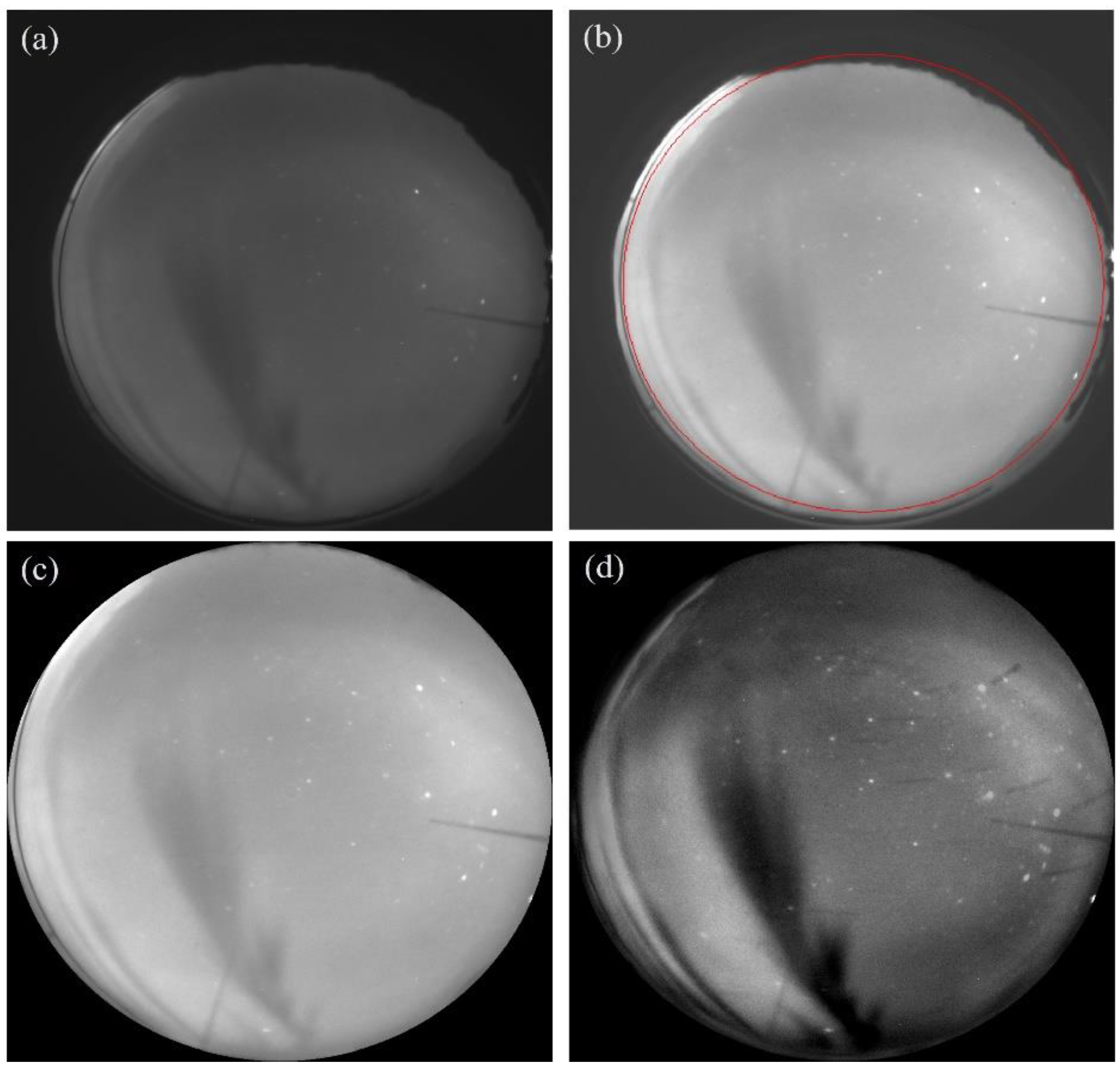
The original airglow image is characterized by low brightness, and the grayscale value of the image is very low. At first, we need to improve the brightness of the original image according to certain rules. Here we use the airglow image at 19:39:20 UT on 2 September 2014, for image enhancement. Figure 2a shows the original airglow image, it is apparent that the original image has low brightness and dynamic range. The brightness of the original image was linearly increased to obtain the enhanced image, as shown in Figure 2b, and the plasma bubble can be observed in Figure 2b. The airglow imager has a large field of view, the optical data around the edge of the airglow image are mostly affected by the local light, and there is a lot of noise. Therefore, the middle part of the image was extracted according to the circular template, and the noise data at the edge of the circular image were removed. Then the smoothed circular airglow image can be obtained, as shown in Figure 2c.

In order to highlight the features of plasma bubbles, it is necessary to remove the background noise from the airglow image. The airglow images for one consecutive hour were selected, there are 20 images in total, and the average image can be obtained by averaging these images. Then, we can take the average image as the background image, subtract the background image from each image, and obtain the processed images with the background noise removed. Finally, the images were normalized to obtain the final enhanced images [21], as shown in Figure 2d, so that the grayscale values of the enhanced image can be distributed in the range of 0–255, and the plasma bubble can be observed more clearly. After these processing steps, clear and high-contrast images of plasma bubbles can be obtained.

2.2. Azimuth Correction

All-sky airglow imagers often do not carry out azimuth calibration when performing optical imaging, so the orientation of an airglow image is generally uncertain. Through azimuth correction, the airglow image with unknown azimuth can be corrected to the right position. Firstly, it is important to find the orientation of the north, which can be identified by the position of the Polaris. Next, we need to figure out the orientations of the east and west. By observing the motion of multiple stars over time, we can obtain the directions of east and west in the airglow image. For the continuous time images, the stars are observed to move from right to left, it can be inferred that the east–west direction is correct, that is, west is on the left and east is on the right, so no flipping is required for east–west orientation. Then, we need to rotate the north to the top of the airglow image, centered on the zenith position, and the rotation angle can be calculated by Equation (1) as follows. In Equation (1), (X_n, Y_n) represents the coordinates of Polaris in the airglow image, (X₀, Y₀) refers to the coordinates of the zenith in the image, and ${\alpha }_N$ is the azimuth of Polaris, which can be obtained through the software Stellarium. Moreover, the nearest interpolation method is adopted to obtain the corrected image; thus, the azimuth correction of the airglow image is accomplished.

$$\theta =-\arctan \frac{X_0-X_n}{Y_0-Y_n}-{\alpha }_N$$

(1)

2.3. Image Projection

To further analyze the main features of plasma bubbles, image projection is required to obtain the final projected image. According to the geographic mapping algorithm, the airglow image can be projected to the corresponding geographic latitude and longitude. In this study, plasma bubbles were observed using airglow emissions at 630 nm wavelength, generally located at an altitude of 250–300 km; thus, the airglow altitude was assumed to be 300 km [21], and the airglow image would be projected to the geographic coordinates at 300 km, and the projection rules can be obtained through the parameter information of the stars in the image. The image projection used in this study is similar to the projection method from Wu’s study, the airglow image was also projected to the altitude of 300 km [14]. In the process of image projection, multiple stars that were evenly distributed in an airglow image were selected, and their elevation angle, azimuth angle, and positions were recorded.

Above all, it is necessary to find the relationship between the incident angle and the image radius of the stars, the incident angle (the zenith angle) is the complement of the elevation angle, and the image radius stands for the pixel distance from the stars to the zenith, and their relationship can be obtained by polynomial fitting, as shown in Equation (2).

$$R\_img=f(\mathrm{zenith})=b+k_1\alpha +k_2{\alpha }^2+k_3{\alpha }^3+\dots$$

(2)

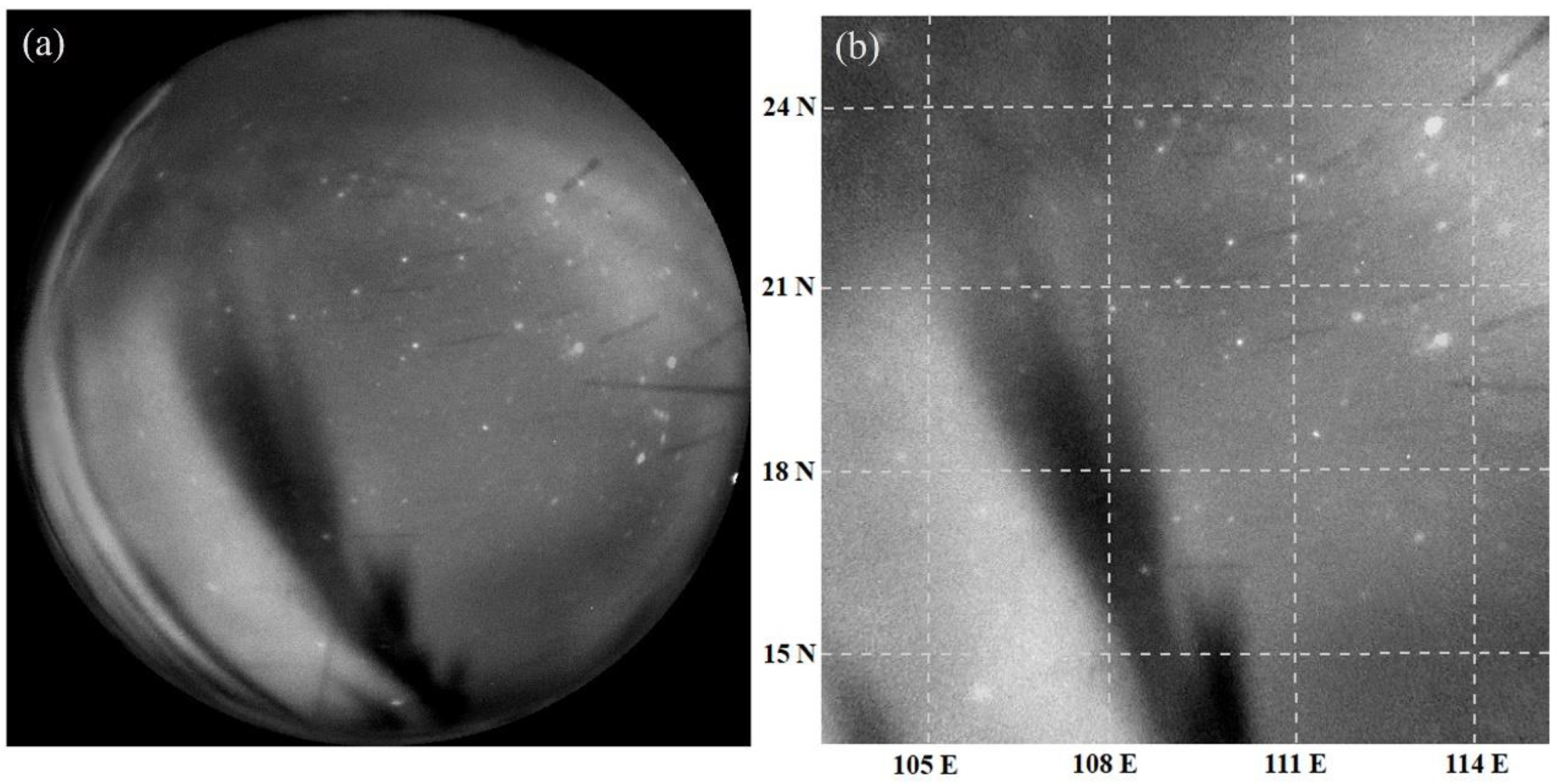
The image projection is finally completed by projecting airglow images to the corresponding geographic coordinates. Figure 3a shows the corrected image at 19:39:20 UT on 2 September 2014, and Figure 3b is the obtained projected image. For the projected image in Figure 3b, the range of latitude and longitude is (13.5°–25.48° N, 103.22°–115.2° E), with per-pixel 0.02°. Fuke station (19.5° N, 109.2° E) is located at the center of the projected image, which also represents the zenith position, and its geomagnetic latitude is 9.9° N.

3. Analysis of the Main Characteristics of Plasma Bubbles

3.1. Morphology and Spatial Scale of Plasma Bubbles

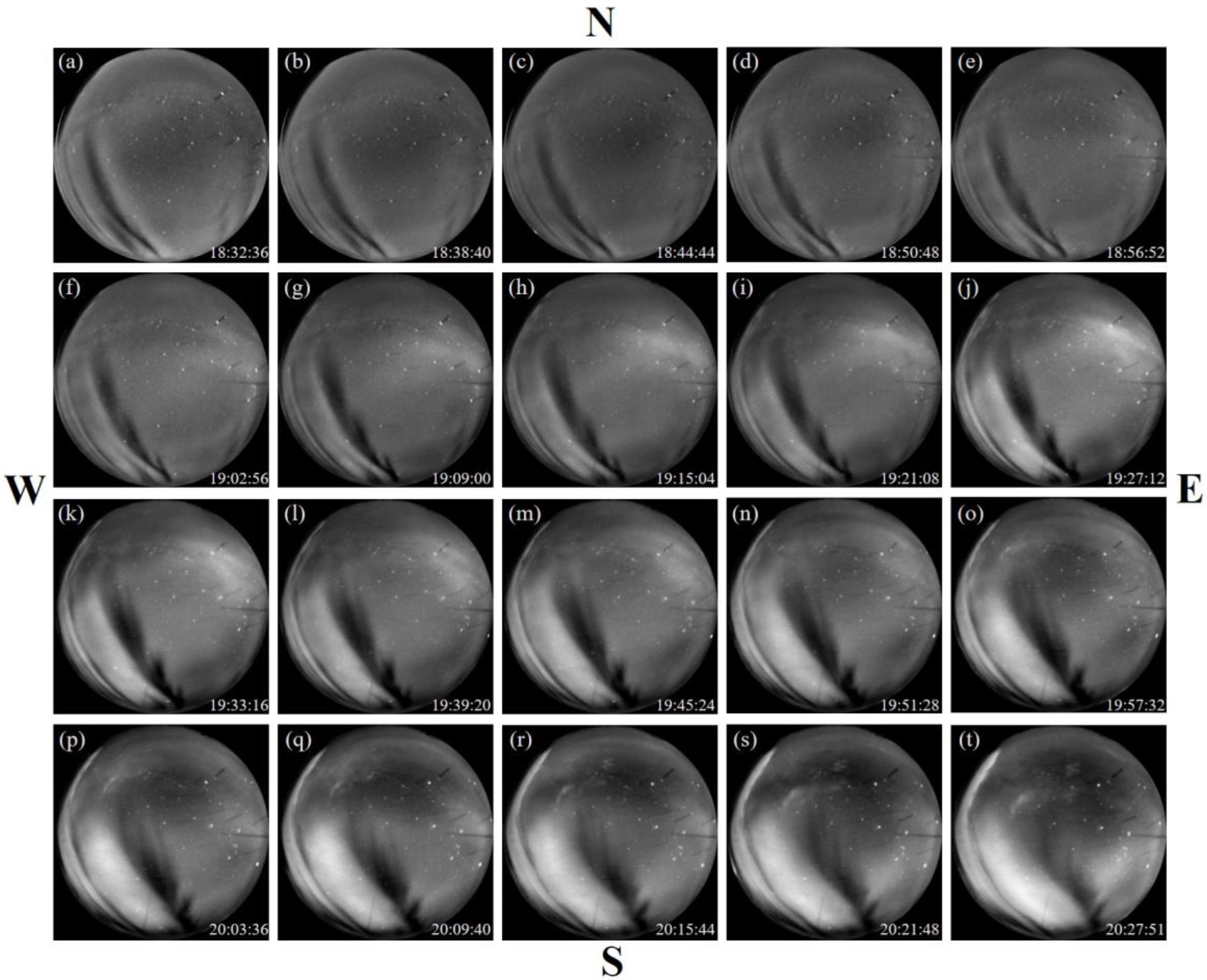
Based on the image processing method of airglow data, as introduced above, we performed image processing on the original airglow images and obtained the clear and recognizable image products of equatorial plasma bubbles (EPBs). Then, the morphological characteristics and temporal–spatial variations of EPBs were analyzed and studied. For the optical images on the evening of 2 September 2014, image processing was performed on these data, and the corrected and projected images of EPBs can be obtained. Figure 4 presents the corrected airglow images of EPB from 18:32:36 UT to 20:27:51 UT, which shows the evolution of EPB from its beginning to its disappearance; the time interval of each subgraph is 6 min. From Figure 4a, EPB exhibits a smaller scale when EPB starts to appear, and EPB shows the shape of a long stripe. With the increase in local time, the spatial scale of the EPB gradually becomes larger. When EPB evolves to a larger scale, EPB is observed as plume-shaped structures and develops into plume irregularities. Moreover, it is visible from Figure 4 that EPB tilts westward as a whole, compared with its north–south distribution, and EPB extends to a long distance along the geomagnetic field lines.

As the EPB scale increases gradually, it can be seen from Figure 4 that a bifurcation phenomenon occurs at the top of the EPB, for example, at 19:15:04 UT in Figure 4h. With the change in time, it is found that the degree of EPB bifurcation increases gradually, and the bifurcation of EPB becomes more pronounced with time. The east wall of the EPB gradually expands outwards over time, and the bifurcation point gradually extends from the top to the bottom of the EPB. Moreover, a small branch appears at the bottom of the EPB, starting from about 19:02:56 UT in Figure 4f, then the small branch gradually separates from the EPB, and becomes more apparent on the east wall of EPB. From Figure 4, the west wall of EPB is relatively stable during this period, while there are some bifurcations on the east wall of EPB. From these observations, it can be inferred that the east wall of EPB is more unstable than the west wall, and we speculate about the possible causes of this phenomenon. The ionospheric irregularities and the neutral wind move eastward together at night, and the plasma density in the EPB is lower than that in the surrounding ionosphere. The interaction between the ions in the EPB will be weakened, so that the velocity of neutral wind in the EPB will be slightly increased, and the extra momentum will affect the east wall of the EPB, which will be correspondingly expanded. For the EPB occurrence on 2 September 2014, it is found that EPB lasts more than 2 h. When the EPB is about to disappear, the intensity gradually weakens over 30 min until the bubble finally disappears.

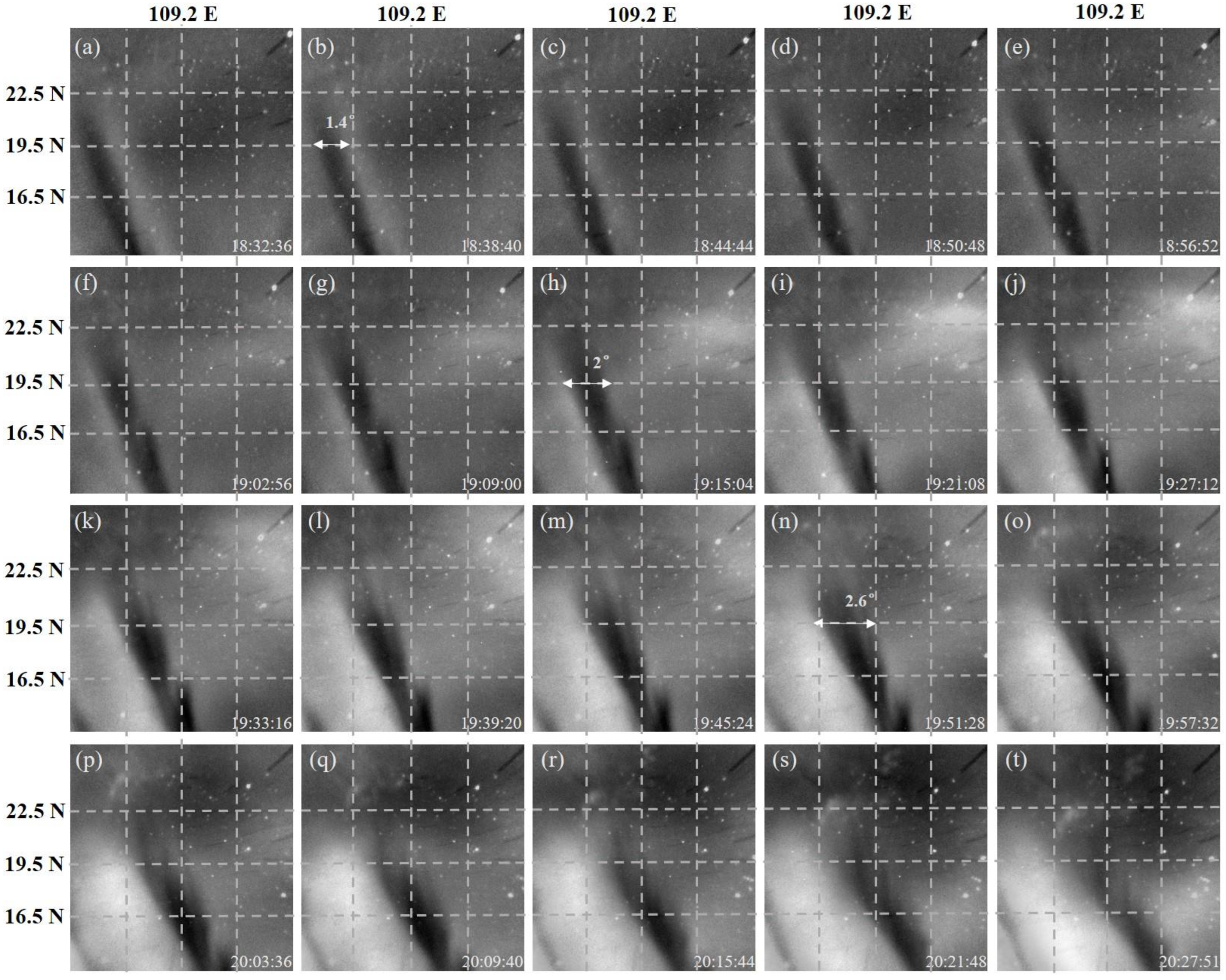
Figure 5 shows the projected images of EPB changing with time on 2 September 2014; these are the results of airglow images after image enhancement, azimuth correction, and image projection. According to the projected images of EPB, the east–west scale of the EPB was analyzed. The EPB scale can be calculated through the longitude range of the EPB in the zenith direction, that is, the horizontal axis at the center of the projected image. In Figure 5b, the EPB spans a longitude of 1.4°, and the east–west scale of EPB is about 165 km at 18:38:40 UT. In Figure 5h, the longitude span of the EPB is 2°; thus, the width of EPB is calculated to be about 240 km at 19:15:04 UT. With the increase in local time, the longitude span of the EPB changes to 2.6° at 19:51:28 UT, and the EPB scale increases to 307 km, as shown in Figure 5n. It can be concluded that the spatial scale of EPB gradually increases with time. At the start of EPB occurrence, EPB appears on a smaller scale. As time goes on, EPB gradually broadens in the east–west direction, and the EPB scale gradually becomes larger over time. The analysis indicates that the east–west scale of EPB is about several hundred kilometers, which is consistent with the results of F-layer irregularities observed by VHF radar [22].

3.2. Drift Velocity of Plasma Bubbles

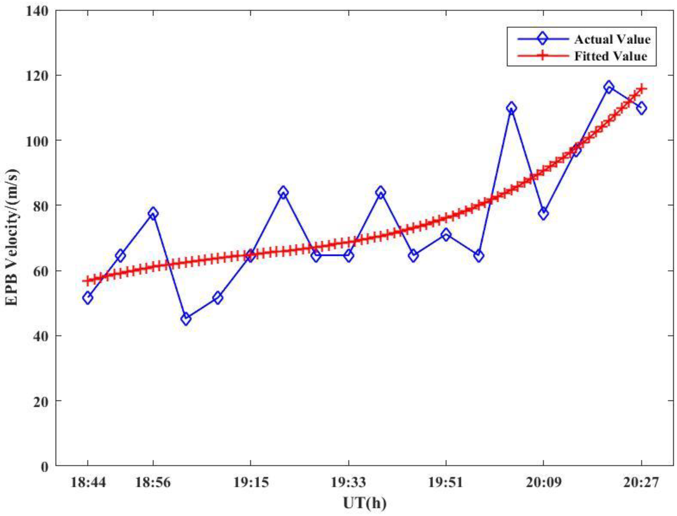
Through analyzing the sequence images of the EPB changing with time, as shown in Figure 5, it can be observed that the EPB exhibits the features of drifting eastward, then the eastward drift velocity of EPB was analyzed and investigated. Here, we use the following method to obtain the drift velocity of EPB, the drift distance of EPB can be calculated through projected images from Figure 5, and the interval time of each image was recorded, then the drift velocity can be obtained through drift distance and interval time. In this study, the airglow data used to analyze the drift velocity began from 18:44 UT to 20:27 UT on 2 September 2014. The west wall of EPB is more stable than the east wall; thus, the drift velocity of the west wall was calculated, which can be appropriate for analyzing the drift velocity of EPB. Figure 6 shows the drift velocity results of EPB changing with time.

In Figure 6, the blue plot shows the actual drift velocity of the EPB, and the red plot represents the fitting results of the drift velocity, which is fitted by a cubic polynomial. It is visible from Figure 6 that the drift velocity of EPB is relatively stable, it fluctuates within a certain range. During the early period of EPB appearance, the EPB exhibits a small drift velocity, about 50 m/s at 18:44 UT. With the increase in local time, the drift velocity of EPB increases gradually, and then reaches a relatively stable condition. During the period of 19:15–19:51 UT, the drift velocity of EPB tends to be more stable, the value of drift velocity is about 70 m/s. When EPB is about to disappear, the drift velocity of EPB continues to increase with time, and the maximum drift velocity reaches about 120 m/s. From Figure 6, it can be concluded that the average drift velocity of the EPB is about 76 m/s (+/−20 m/s), and the drift velocity of the EPB is in the range of 40–130 m/s (+/−20 m/s).

4. Statistical Analysis of the Occurrence of Plasma Bubbles

Based on the airglow observation data over a long period, the occurrence of plasma bubbles can be analyzed and studied. The data used to do the statistical analysis in Fuke began from 1 September 2014 to 31 August 2015. The image processing method was used to process these optical data, and clear and recognizable images of plasma bubbles can be obtained. Then we made a statistical analysis of the occurrence of equatorial plasma bubbles (EPBs), and investigated the monthly and seasonal variations of EPB occurrence.

4.1. Statistical Analysis of the Monthly Occurrence of Plasma Bubbles

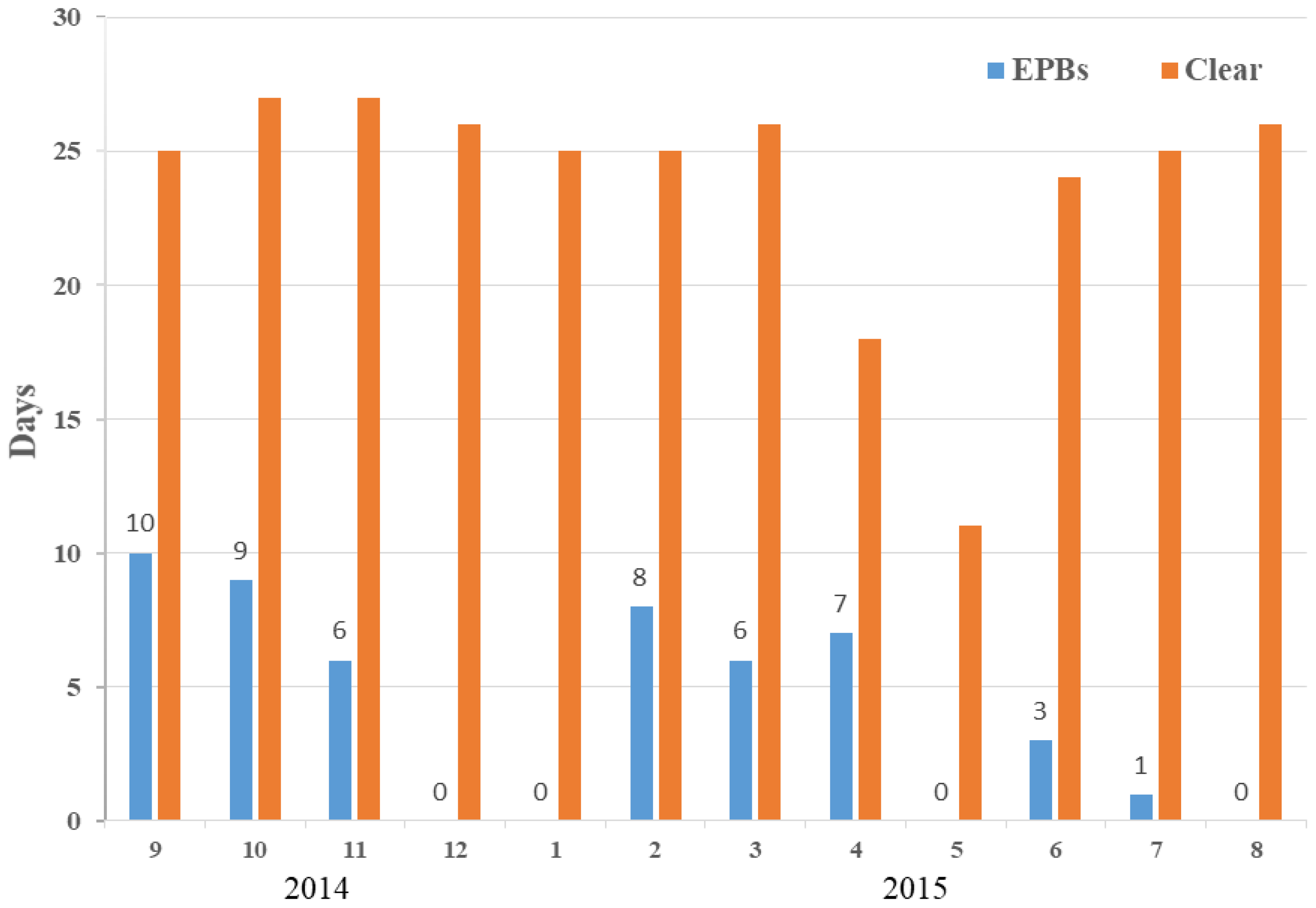
Using the airglow data from September 2014 to August 2015, we statistically analyzed the monthly occurrence of plasma bubbles. Through the statistics of optical data during this period, we obtained the numbers of EPB days and clear days per month, and the statistical features of EPB occurrence with months were analyzed. In the process of data statistics, the situation that the clear period at night exceeded 1 h was marked as a clear night. Figure 7 shows the statistical distribution histogram of EPB days and clear days in each month.

Figure 7 gives the statistical results of EPB days and clear days every month. The total numbers of observation days in Fuke are 330 from September 2014 to August 2015, and the optical observation was almost carried out every day in most months of the year. From Figure 7, EPBs occur most frequently in September 2014, with 10 events. The rest of fall in October and November generally have decreasing occurrence than September, with 9 and 6 events, respectively, followed by EPB occurrence in the early–mid winter. Occurrence increases again in late winter and spring, followed by a small peak in early summer. To conclude, EPBs appear more frequently from September to November 2014 and February to April 2015.

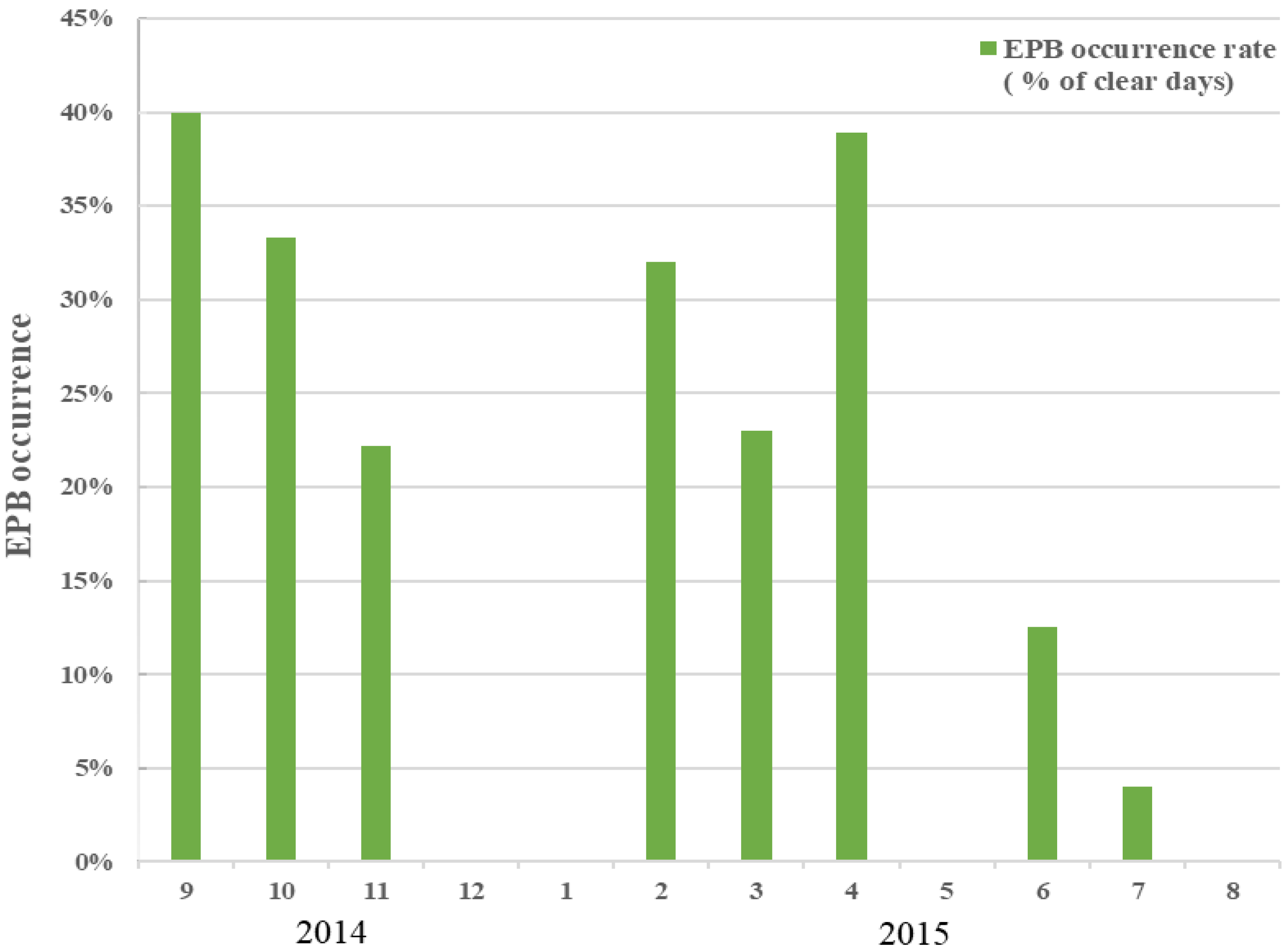
Therefore, the occurrence rate of EPBs in each month can be calculated and obtained. In this study, the occurrence rate is the percentage of clear days with EPB, Figure 8 presents the statistical results of the monthly occurrence rate of EPBs over the period from September 2014 to August 2015.

Figure 8 shows the statistical distribution histogram of EPB occurrence in each month, the green bar represents the EPB occurrence rate. From Figure 8, EPBs mainly occur from September to November in 2014, and from February to April in 2015. The maximum occurrence rate is 40% in September. Then followed by April, the occurrence rate of EPBs is also relatively higher, reaching 38%. EPBs also show a high occurrence rate in October and February, which are both close to 33%. Figure 8 shows that the EPB occurrence rate is very low from December to January, the occurrence rate is 0 in these months. In addition, EPBs are less observed during the period from June to July 2015, and the calculated occurrence rate is relatively lower, which is less than 15%. In conclusion, EPBs occur more frequently during the months of September to November and February to April, for the twelve months observed. However, the occurrence rate of EPBs is relatively low in other months.

4.2. Statistical Analysis of the Seasonal Occurrence of Plasma Bubbles

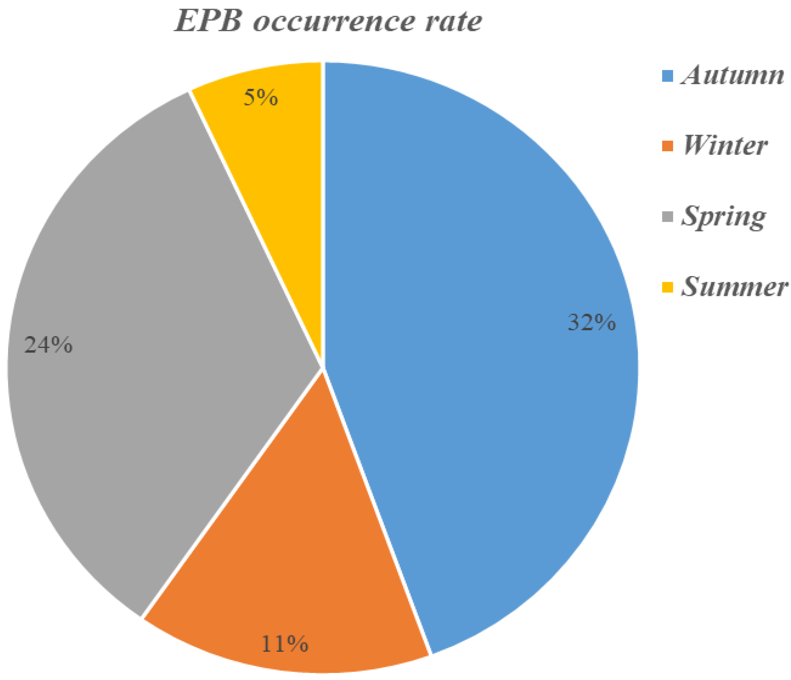
Considering the seasonal occurrence of EPBs, based on the airglow data from autumn 2014 to summer 2015, we made statistics on the seasonal occurrence of EPBs. For the seasonal statistics of airglow data, we set March to May as spring, June to August as summer, September to November as autumn, and December to February as winter. Figure 9 shows the statistical results of the seasonal occurrence rate of EPBs from September 2014 to August 2015.

Figure 9 presents the pie chart of seasonal statistics of EPB occurrence rate. From Figure 9, EPBs have the highest occurrence rate in autumn, reaching 32%, followed by spring, with an occurrence rate of 24%. Next is winter, the EPB occurrence rate is 11%, and the lowest in summer, with 5%. According to Figure 9, we can conclude that EPBs tend to occur more frequently in spring and autumn, with a high occurrence rate, while EPBs can be less observed in summer and winter.

Through the statistical analysis of airglow data from autumn 2014 to summer 2015, it can be extrapolated that plasma bubbles will mainly occur in spring and autumn for a given year. Plasma bubbles are the main cause of scintillations in the ionosphere [21,22], GPS scintillation data can be used to analyze and study the variation and occurrence of plasma bubbles [11]. The appearance and development of plasma bubbles can be closely related to ionospheric scintillations [23]; thus, ionospheric scintillations also appear more likely in spring and autumn.

5. Discussion

Through the analysis of the main features of EPBs in Hainan, it is found that EPB exhibits plume-shaped irregularities in morphology. The spatial scale of the EPB gradually increases with time, and EPB gradually becomes wider in the east–west direction. Moreover, the EPB scale is about hundreds of kilometers, which is similar to the results of radar observations. Optical observation results indicate that EPB exhibits the characteristics of westward tilt. Previous studies show that EPBs often tilt westward in most cases [15,21], which may be caused by plasma drift shear [24]. With the increase in time, it is observed that a bifurcation appears at the top of the EPB, the bifurcation becomes more pronounced with time, which is similar to other events [13,21]. Moreover, it is found that there are some bifurcations on the east wall of EPB, the EPB bifurcation is not apparent at the beginning. Afterwards, the branches of the east wall gradually spread outwards over time, the degree of bifurcation gradually increases with time, and the bifurcation phenomenon becomes more obvious. This phenomenon may be due to the instability of the east wall of EPB [14]. In terms of the studies on EPB bifurcation, Carrasco et al. [20] investigated the generation and evolution of plasma bubbles by simulating the EPB, explained the physical mechanism for the EPB bifurcation, and conclude that the variation of the polarization electric fields inside the bubble makes an important influence on the bifurcation mechanism.

Optical observations show that EPB has the features of eastward drift, and the drift velocity of EPB is about 40–130 m/s (+/−20 m/s), which is close to the previous studies of the EPB drift velocity in Hainan, the drift speed of EPB is typically 50–150 m/s [21,25]. In terms of the seasonal variation of EPB occurrence, the statistical results show that EPBs have a high occurrence rate in spring and autumn, and EPBs generally appear less in winter and summer. Wu et al. reported that EPBs mainly appeared in the months of September–October and February–April [14], and the typical seasons for EPB occurrence are spring and autumn. Sun et al. also revealed that EPBs tend to occur in spring and autumn [15]; our findings are consistent with their studies on the EPB occurrence.

6. Conclusions

Based on optical data acquired by the all-sky airglow imager in Fuke, Hainan (geomagnetic latitude = 9.9° N), we utilized an image processing method to process the original airglow data, including image enhancement, azimuth correction, and image projection, and obtained the clear and recognized image products of plasma bubbles. We selected the airglow data of plasma bubbles on the evening of 2 September 2014, and then analyzed the main optical characteristics of plasma bubbles, such as morphology, spatial scale, drift features, etc. Moreover, we employed nearly one year of airglow data (from 1 September 2014 to 31 August 2015) from the all-sky airglow imager in Fuke, and made a statistical analysis of the occurrence of plasma bubbles. In the statistics, we investigated the monthly and seasonal occurrence rates of plasma bubbles during one year, and obtained the statistical characteristics of the occurrence of plasma bubbles. Plasma bubbles generally have a significant impact on high-frequency (HF) communications, satellite-ground communications, and GPS navigation and positioning. Therefore, it is of great scientific significance to further investigate equatorial plasma bubbles (EPBs) at low latitudes, which can be beneficial to the forecasting of ionospheric scintillations. The main conclusions and findings in this study are presented as follows.

(1)

For the optical observation of EPB on September 2 in 2014, it is found that EPB usually appears as plume-shaped structures in morphology, EPB often tilts to the west as a whole, compared with its north–south distribution, and EPB extends to a long distance along the geomagnetic field lines. It is found that the spatial scale of the EPB gradually increases over time. As the EPB increases to a larger scale, EPB shows the features of a vertical bifurcation, the bifurcation of EPB becomes more pronounced with time, and the bifurcation point gradually extends from the top to the bottom of the EPB. The observation results show that the west wall of EPB is relatively more stable, while there are some bifurcations on the east wall of EPB. Moreover, when EPB is about to disappear, the intensity of EPB gradually weakens until EPB finally disappears;

(2)

According to the projected images of EPB, the spatial scale and drift velocity of EPB were analyzed and studied. During the early period of EPB occurrence, EPB appears on a smaller scale. With the increase in time, EPB gradually widens in the east–west direction, the EPB scale gradually increases with time. It can be obtained that the east–west scale of EPB is about several hundred kilometers. In our observations, EPB exhibits the features of drifting eastward. The analysis indicates that the drift velocity of EPB increases gradually with time, and then reaches a relatively stable condition. It is concluded that the drift velocity of the EPB is in the range of 40–130 m/s (+/−20 m/s), and the average drift velocity of the EPB is about 76 m/s (+/−20 m/s);

(3)

Based on the airglow observation data for one year, we investigated the statistical features of the occurrence of EPBs. The statistical results show that EPBs mainly appear in the months of September–November and February–April. The occurrence rate of EPBs presents the highest in September, reaching 40%, and EPBs are less observed from June to July 2015, and the occurrence rate is less than 15% in the two months. Considering seasonal occurrence, EPBs in the ionospheric F-region tend to occur more frequently in spring and autumn, while rarely being observed in summer and winter. The statistical results show occurrence rates of 32 % in autumn, the highest of the year, followed by 24 % for spring, 11 % for winter, and the lowest of the year, 5 % in summer.

References

- Kelley, M.C. The Earth’s Ionosphere: Plasma Physics and Electrodynamics; Academic Press: San Diego, CA, USA, 1989. [Google Scholar]
- Sultan, P.J. Linear theory and modeling of the Rayleigh-Taylor instability leading to the occurrence of equatorial spread F. J. Geophys. Res. Space Phys. 1996, 101, 26875–26891. [Google Scholar] [CrossRef]
- Kelley, M.C.; Makela, J.J.; Ledvina, B.M.; Kintner, P.M. Observations of equatorial spread-F from Haleakala, Hawaii. Geophys. Res. Lett. 2002, 29, 64-1–64-4. [Google Scholar] [CrossRef]
- Makela, J.J. A review of imaging low-latitude ionospheric irregularity processes. J. Atmos. Sol.-Terr. Phys. 2006, 68, 1441–1458. [Google Scholar] [CrossRef]
- Woodman, R.F.; Hoz, C.L. Radar observations of F region equatorial irregularities. J. Geophys. Res. 1976, 81, 5447–5466. [Google Scholar] [CrossRef]
- Taori, A.; Sindhya, A. Measurements of equatorial plasma depletion velocity using 630 nm airglow imaging over a low-latitude Indian station. J. Geophys. Res. Space Phys. 2014, 119, 396–401. [Google Scholar] [CrossRef]
- Narayanan, V.L.; Gurubaran, S.; Shiny, M.B.B.; Emperumal, K.; Patil, P. Some new insights of the characteristics of equatorial plasma bubbles obtained from Indian region. J. Atmos. Sol. Terr. Phys. 2017, 156, 80–86. [Google Scholar] [CrossRef]
- Hickey, D.A.; Martinis, C.R. All-Sky Imaging Observations of the Interaction between the Brightness Wave and ESF Airglow Depletions. J. Geophys. Res. Space Phys. 2020, 125, e2019JA027232. [Google Scholar] [CrossRef]
- Weber, E.J.; Buchau, J.; Eather, R.H.; Mende, S.B. North-south aligned equatorial airglow depletions. J. Geophys. Res. 1978, 83, 712–716. [Google Scholar] [CrossRef]
- Otsuka, Y.; Shiokawa, K.; Ogawa, T.; Wilkinson, P. Geomagnetic conjugate observations of equatorial airglow depletions. Geophys. Res. Lett. 2002, 29, 43-1–43-4. [Google Scholar] [CrossRef]
- Makela, J.J.; Ledvina, B.M.; Kelley, M.C.; Kintner, P.M. Analysis of the seasonal variations of equatorial plasma bubble occurrence observed from Haleakala, Hawaii. Ann. Geophys. 2004, 22, 3109–3121. [Google Scholar] [CrossRef] [Green Version]
- Tardelli-Coelho, F.; Pimenta, A.A.; Tardelli, A.; Abalde, J.; Venkatesh, K. Plasma blobs associated with plasma bubbles observed in the Brazilian sector. Adv. Space Res. 2017, 60, 1716–1724. [Google Scholar] [CrossRef]
- Gurav, O.B.; Narayanan, V.L.; Sharma, A.K.; Ghodpage, R.N.; Gaikwad, H.P.; Patil, P.T. Airglow imaging observations of some evolutionary aspects of equatorial plasma bubbles from Indian sector. Adv. Space Res. 2019, 64, 385–399. [Google Scholar] [CrossRef]
- Wu, Q.; Yu, T.; Lin, Z.X.; Xia, C.L.; Zuo, X.M.; Wang, X. Night airglow observations to irregularities in the ionospheric F region over Hainan. Chin. J. Geophys. 2016, 59, 17–27. [Google Scholar]
- Sun, L.; Xu, J.; Wang, W.; Yuan, W.; Li, Q.; Jiang, C. A statistical analysis of equatorial plasma bubble structures based on an all-sky airglow imager network in China. J. Geophys. Res. Space Phys. 2016, 121, 11495–11517. [Google Scholar] [CrossRef]
- Sahai, Y.; Aarons, J.; Mendillo, M.; Baumgardner, J.; Bittencourt, J.; Takahashi, H. OI 630 nm imaging observations of equatorial plasma depletions at 16°S dip latitude. J. Atmos. Sol. Terr. Phys. 1994, 56, 1461–1475. [Google Scholar] [CrossRef]
- Sahai, Y.; Fagundes, P.R.; Bittencourt, J.A. Solar cycle effects on large scale equatorial F-region plasma depletions. Adv. Space Res. 1999, 24, 1477–1480. [Google Scholar] [CrossRef]
- Abalde, J.R.; Fangundes, P.R.; Bittencourt, J.A.; Sahai, Y. Observations of equatorial F region plasma bubbles using simultaneous OI 777.4 nm and OI 630.0 nm imaging: New results. J. Geophys. Res. 2001, 106, 30331–30336. [Google Scholar] [CrossRef]
- Hosokawa, K.; Takami, K.; Saito, S.; Ogawa, Y.; Otsuka, Y.; Shiokawa, K.; Chen, C.-H.; Lin, C.-H. Observations of equatorial plasma bubbles using a low-cost 630.0-nm all-sky imager in Ishigaki Island, Japan. Earth Planets Space 2020, 72, 1–11. [Google Scholar] [CrossRef]
- Carrasco, A.J.; Pimenta, A.A.; Wrasse, C.M.; Batista, I.S.; Takahashi, H. Why Do Equatorial Plasma Bubbles Bifurcate? J. Geophys. Res. Space Phys. 2020, 125, e2020JA028609. [Google Scholar] [CrossRef]
- Ma, X.; Fang, H. Optical observation of plasma bubbles and comparative study of multiple methods of observing the ionosphere over China. Adv. Space Res. 2020, 65, 2761–2772. [Google Scholar] [CrossRef]
- Li, G.; Ning, B.; Abdu, M.A.; Wan, W.; Hu, L. Precursor signatures and evolution of post-sunset equatorial spread-F observed over Sanya. J. Geophys. Res. Space Phys. 2012, 117. [Google Scholar] [CrossRef]
- Li, G.; Ning, B.; Yuan, H. Analysis of ionospheric scintillation spectra and TEC in the Chinese low latitude region. Earth Planets Space 2007, 59, 279–285. [Google Scholar] [CrossRef]
- Zalesak, S.T.; Ossakow, S.L.; Chaturvedi, P.K. Nonlinear equatorial spread F: The effect of neutral winds and background Pedersen conductivity. J. Geophys. Res. Space Phys. 1982, 87, 151–166. [Google Scholar] [CrossRef]
- Chen, Y.H.; Huang, W.G.; Gong, J.C.; Ma, G.Y.; Sun, C.L.; Shen, H. Observations of ionospheric irregularity zonal velocity in Hainan. Chin. J. Space Sci. 2008, 28, 295–300. [Google Scholar]
Figure 1.
Processing steps for airglow images of plasma bubbles.
Figure 2.
Airglow image enhancement for 19:39:20 UT on 2 September 2014. (a) the original airglow image; (b) the enhanced airglow image; (c) the extracted circular airglow image; (d) the normalized airglow image.
Figure 3.
Image correction and projection for 19:39:20 UT on 2 September 2014. (a) the corrected airglow image; (b) the projected airglow image.
Figure 4.
Corrected airglow images from 18 UT to 20 UT on 2 September 2014 (a–t).
Figure 5.
Projected airglow images from 18 UT to 20 UT on 2 September 2014 (a–t).
Figure 6.
Drift velocity of EPB on 2 September 2014.
Figure 7.
Statistical results of EPB days and clear days in each month over Fuke (9.9 degrees MLAT).
Figure 8.
Statistical results of EPB occurrence in each month over Fuke (9.9 degrees MLAT).
Figure 9.
Seasonal statistical results of EPB occurrence over Fuke (9.9 degrees MLAT).
Disclaimer/Publisher’s Note: The statements, opinions and data contained in all publications are solely those of the individual author(s) and contributor(s) and not of MDPI and/or the editor(s). MDPI and/or the editor(s) disclaim responsibility for any injury to people or property resulting from any ideas, methods, instructions or products referred to in the content. |
© 2023 by the authors. Licensee MDPI, Basel, Switzerland. This article is an open access article distributed under the terms and conditions of the Creative Commons Attribution (CC BY) license (https://creativecommons.org/licenses/by/4.0/).
Share and Cite
MDPI and ACS Style
Ma, X.; Wu, M.; Guo, P.; Xu, J. Airglow Observation and Statistical Analysis of Plasma Bubbles over China. Atmosphere 2023, 14, 341. https://doi.org/10.3390/atmos14020341
AMA Style
Ma X, Wu M, Guo P, Xu J. Airglow Observation and Statistical Analysis of Plasma Bubbles over China. Atmosphere. 2023; 14(2):341. https://doi.org/10.3390/atmos14020341
Chicago/Turabian StyleMa, Xin, Mengjie Wu, Peng Guo, and Jing Xu. 2023. "Airglow Observation and Statistical Analysis of Plasma Bubbles over China" Atmosphere 14, no. 2: 341. https://doi.org/10.3390/atmos14020341
Note that from the first issue of 2016, this journal uses article numbers instead of page numbers. See further details here.