Article

Identification of Large-Scale Travelling Ionospheric Disturbances (LSTIDs) Based on Digisonde Observations

by
Ioanna Tsagouri
,
Anna Belehaki
*,
Konstantinos Koutroumbas
,
Konstantinos Tziotziou
and
Themistocles Herekakis
National Observatory of Athens, Institute for Astronomy, Astrophysics, Space Applications and Remote Sensing, 15236 Penteli, Greece
*
Author to whom correspondence should be addressed.
Atmosphere 2023, 14(2), 331; https://doi.org/10.3390/atmos14020331
Submission received: 22 December 2022 / Revised: 26 January 2023 / Accepted: 31 January 2023 / Published: 7 February 2023
(This article belongs to the Special Issue Ionospheric Science and Ionosonde Applications)

Abstract

:
In this paper we analyze Digisonde observations obtained in the European region to specify the effects of large-scale travelling ionospheric disturbances (LSTIDs) on the ionospheric characteristics that define the conditions in the bottomside ionosphere. While this type of disturbances affects all frequency ranges in the F region, the most pronounced effect is detected in the foF2 critical frequency, where the density is the highest. During LSTID activity, a significant uplifting of the F2 layer is observed to accompany an oscillation pattern in the foF2. Concurrent variations in the height of the peak electron density hmF2 and the corresponding scale height, Hm are also observed. These findings are used to propose a new methodology for the identification of LSTIDs, comprising a combination of different criteria. The efficiency of the proposed methodology is tested at middle latitudes during geomagnetically quiet and disturbed intervals as well as during time periods of lower atmosphere forcing affecting the ionosphere.

1. Introduction

Travelling ionospheric disturbances (TIDs) are plasma density fluctuations that propagate as waves through the ionosphere at a wide range of velocities and frequencies and play an important role in the exchange of momentum and energy between various regions of the upper atmosphere. TIDs are the ionospheric manifestation of internal atmospheric gravity waves (AGWs) in the neutral atmosphere [1,2] associated with auroral and geomagnetic activity and with lower atmosphere phenomena of non-space origin (e.g., severe tropospheric convection or passages of cold fronts, seismicity, volcanic activity, and artificially triggered events such as explosions). Independent of their source, the effects imposed by TIDs at the ionospheric altitudes are very important. It is now confirmed that TIDs constitute a threat for operational systems using predictable ionospheric characteristics, as they can impose disturbances with amplitudes of up to ~20% of the ambient electron density, a Doppler frequency shift of the order of 0.5 Hz on HF signals [3] and perturbations in the total electron content (TEC) that range from less than 1 up to 10 TEC units (TECU) [4]. Small amplitude TIDs, occurring virtually all the time, similar to cloud occurrence in the troposphere, can tilt the reflecting iso-density contours by as much as 3° to 5°. These time-varying tilts cause variances in the measured bearings of about 1° for emitter distances of 1000 km to about 100° for 100 km, the “short-range catastrophe” [5]. The accuracy of ground-based single-site-location (SSL) HF radio wave direction-finding is severely compromised by the passage of TIDs through the ionospheric reflection area. TIDs of larger amplitudes affect the performance of global navigation satellite systems (GNSS), and in particular, satellite based augmentation Systems (SBAS), such as the European SBAS EGNOS [6], since associated variations in total electron content of several TECU may decrease the observed accuracy and limit the availability of these systems for the different applications they support (mainly aviation). On the other hand, short-scale TIDs affect the performance of high-accuracy navigation systems, such as network real-time kinematic (N-RTK), given that differential ionospheric errors greater than 34 cm (2 TECU) cause problems in high precision differential Global Position System (GPS) applications [4]. In fact, TIDs are considered a nuisance for any system using trans-ionospheric propagation, such as trans-ionospheric radio astronomical observations at low frequencies (10–250 MHz). TIDs remain a troubling cause of coordinate registration (CR, geolocation) errors. They are also the principal mechanism limiting the performance of target detection algorithms for geolocation systems, because the associated range/azimuth deflections spread the target return in the algorithm results [7].
Large-scale travelling ionospheric disturbances (LSTIDs) are generally considered to be the ionospheric manifestation of AGWs that are associated with auroral and geomagnetic activity [1,8,9,10,11]. Auroral processes considered to generate LSTIDs [1,12] include Joule heating and Lorentz forces caused by the enhancement of the auroral electrojet or intense precipitation of charged particles among the main excitation sources of the LSTIDs. Enhanced thermospheric heating and wind launch waves propagating away from the auroral oval as gravity waves, and ion drag creates the ionosphere density perturbation [13,14,15,16]. These disturbances have typical horizontal velocities between 300 and 1000 m/s, horizontal wavelengths of more than 1000 km, and period in the range of 30 min to 3 h [8,9]. In general, in the northern hemisphere, LSTIDs have a south to south–east propagation direction, as they are generated in the northern auroral zone. Rare cases of poleward propagating LSTIDs have been observed either in connection with energy dissipation from medium scale TIDs (MSTIDs) of lower atmosphere origin [17] or in connection with interhemispheric constructive interference [18]. The physics behind LSTIDs remains not fully understood. Indicative open issues include: the exact physical mechanisms for LSTIDs formation, including transformation of various types of energy within the magnetosphere–ionosphere–thermosphere system; the trigger mechanisms of releasing the stored energy; the basic properties and parameters of LSTIDs and their propagation direction from the source; the way they dissipate with distance; and the effect of background ionospheric conditions on their propagation.
MSTIDs are mostly associated with the ionospheric coupling with the lower atmosphere and have no clear correlation with geomagnetic activity. Ionospheric plasma perturbations with horizontal wavelength of ~100–500 km are considered to be MSTIDs. Phase speed and period of MSTIDs are 250–1000 m/s and 15 min to 1 h, respectively [1]. MSTIDs are observed both during the daytime and nighttime, but the causative mechanisms of daytime and nighttime MSTIDs are different [19]. Investigations suggest that daytime MSTIDs are generated in association with primary and/or secondary gravity waves [20] mainly originating in the lower and middle atmosphere, respectively. On the other hand, the nighttime MSTIDs are caused by electrodynamical processes, i.e., Perkins instability associated with E- and F-region coupling processes [21,22]. Furthermore, the MSTIDs’ climatology has a proven dependence on the longitude.. Several physical processes are proposed to be connected with the climatological behavior of MSTIDs, such as polar atmospheric processes, particularly polar vortex variabilities, and stratospheric winds, and also, sporadic E layers and interhemispheric coupling [20,23,24,25,26].
On the other hand, dynamic phenomena of sporadic nature and, especially, earthquakes trigger ionospheric perturbations generated by different sub-sources and can be distinguished by their propagation speed (see for example [27]). Disturbances associated with acoustic waves generated by the crustal motion propagate at 600–1000 m/s; disturbances generated by Rayleigh surface waves have speeds similar to those of the source waves on the ground, that is, 3.3–4 km/s [28]. These different disturbances’ components can be seen well in detrended TEC maps, in iso-ionic contour plots, and in continuous Doppler sounding system (CDSS) recordings.
Due to the wide range of the TIDs’ impact on technological systems, the specification of TID activity over large world regions is a key requirement for the operation of systems using or affected by the ionosphere. However, the limitations in present understanding of their generation and propagation mechanisms make tracking and even nowcasting of TIDs a very challenging task. To help relevant efforts, in the following sections, we analyze ionospheric observations obtained by ground-based ionosondes at middle latitudes, aiming at the determination of the key characteristics and behavior of LSTIDs in the bottomside ionosphere. The ultimate goal is to propose a new methodology for the identification of LSTIDs based on ionospheric characteristics that are routinely monitored by Digisondes, and, therefore, can potentially support operational implementation.
The structure of the paper is as follows:
  • Data and methods are presented in Section 2.
  • The results are given in Section 3:
    Disturbances in ionospheric characteristics relevant to LSTIDs are analyzed and specified in Section 3.1.
    A set of criteria for the detection of LSTIDs is proposed in Section 3.2
    The LSTID detection criteria are applied over intervals with different geophysical characteristics, including solar and lower atmosphere forcing, in Section 3.3.
  • The results are discussed in Section 4.
  • Some conclusive remarks are provided in Section 5.

2. Data and Methods

To specify the effects of LSTIDs within the parameters that define the shape of the electron density profile, we analyzed iso-ionic height data at the frequency range of 2–8 MHz; and critical ionospheric characteristics, such as the foF2, the hmF2, and the scale height at hmF2, Hm, which is the vertical distance in which the electron density decreases by a factor of e. Considering that LSTIDs are caused by the movement of plasma up and down in the inclined magnetic field due to meridional winds, resulting changes in altitude were assumed to be most pronounced in the “reduced height” hmF2-ho, where ho is the height of the peak density for overhead sun. For the purpose of this analysis, ho was estimated to be equal to 200 km, based on the daily variation of the monthly median values of the hmF2 derived from several Digisonde stations, presented in the subsequent plots. Data derived from vertical incidence ionograms were obtained by three European Digisondes with 5 min cadence: Athens (38° N, 23.5° E), Dourbes (50.1° N, 4.6° E) and Ebre (40.8° N, 0.5° E). The data were retrieved from the Global Ionosphere Radio Observatory (GIRO—http://giro.uml.edu/, accessed on 14 January 2023) data repository [29]. To ensure the highest quality of observations, the ionograms analyzed here were manually scaled in all cases. Manually scaling of ionograms was performed using the SAO Explorer software provided with open access in https://ulcar.uml.edu/SAO-X/SAO-X.html (accessed on 25 January 2023). Detrended iso-ionic data dh(f) provided information about local disturbances at the height of HF frequency reflections due to TIDs. The detrending was applied to the five-minute cadence data using a running window of 1 h.
The auroral electrojet Indicators IU and IL derived from the Finnish Meteorological Institute (FMI)—International Monitor for Auroral Geomagnetic Effects (IMAGE) magnetometer chain were also used here as proxies for the magnetospheric activity in the European sector (https://space.fmi.fi/image/www/index.php?page=home, accessed on 14 December 2022). In particular, we analyzed magnetometer data from Norway to test the hypothesis that the observed perturbations are triggered by auroral activity. The list of the magnetometer stations used for the calculation of the IU and IL indicators analyzed here are provided in Table 1, together with their geographic coordinates. The geomagnetic activity level was assessed through records of the Dst index available from the World Data Center (WDC) for Geomagnetism, Kyoto (http://wdc.kugi.kyoto-u.ac.jp/dstdir/, accessed on 14 January 2023).
The analysis includes periods of both quiet and enhanced geomagnetic activity that occurred from 2020 until 2022.

3. Results

3.1. LSTID Identification Based on the Analysis of Ionospheric Characteristics

In this part of the analysis, we present indicative results for the interval from 24 to 30 September 2020 that is characterized by weak to moderate geomagnetic activity. The Dst index for this time interval is presented in the top panel of Figure 1. The response of the ionospheric characteristics foF2 and hmF2 with respect to monthly median conditions, as well as the scale height (Hm) and the “reduced height” (hmF2–200) from 24 to 30 September 2020 over Athens, are also presented in Figure 1 (second to forth panels, respectively). A feature of particular interest of this response, indicative of LSTID activity over Athens, is the quasi-oscillations in the foF2 characteristic that are mainly observed during daytime hours (especially on 24–26 September) and are often accompanied by uplifting of the F2 layer.
Next, we analyzed the perturbations recorded on 24 September 2020, the day with the most pronounced oscillations in foF2. From top to bottom, Figure 2 presents the auroral electrojet indicators IU and IL; the detrended iso-ionic heights for the frequency range 2.0 to 7.8 MHz; the variation of the cut-off frequency foF2 with its monthly median (foF2_m); the variation of the true height (hmF2) with respect to its monthly median values (hmF2_m); and the scale height at hmF2 (Hm) together with the variation of the parameter (hmF2-200). Overall, two periods of important perturbation are discerned:
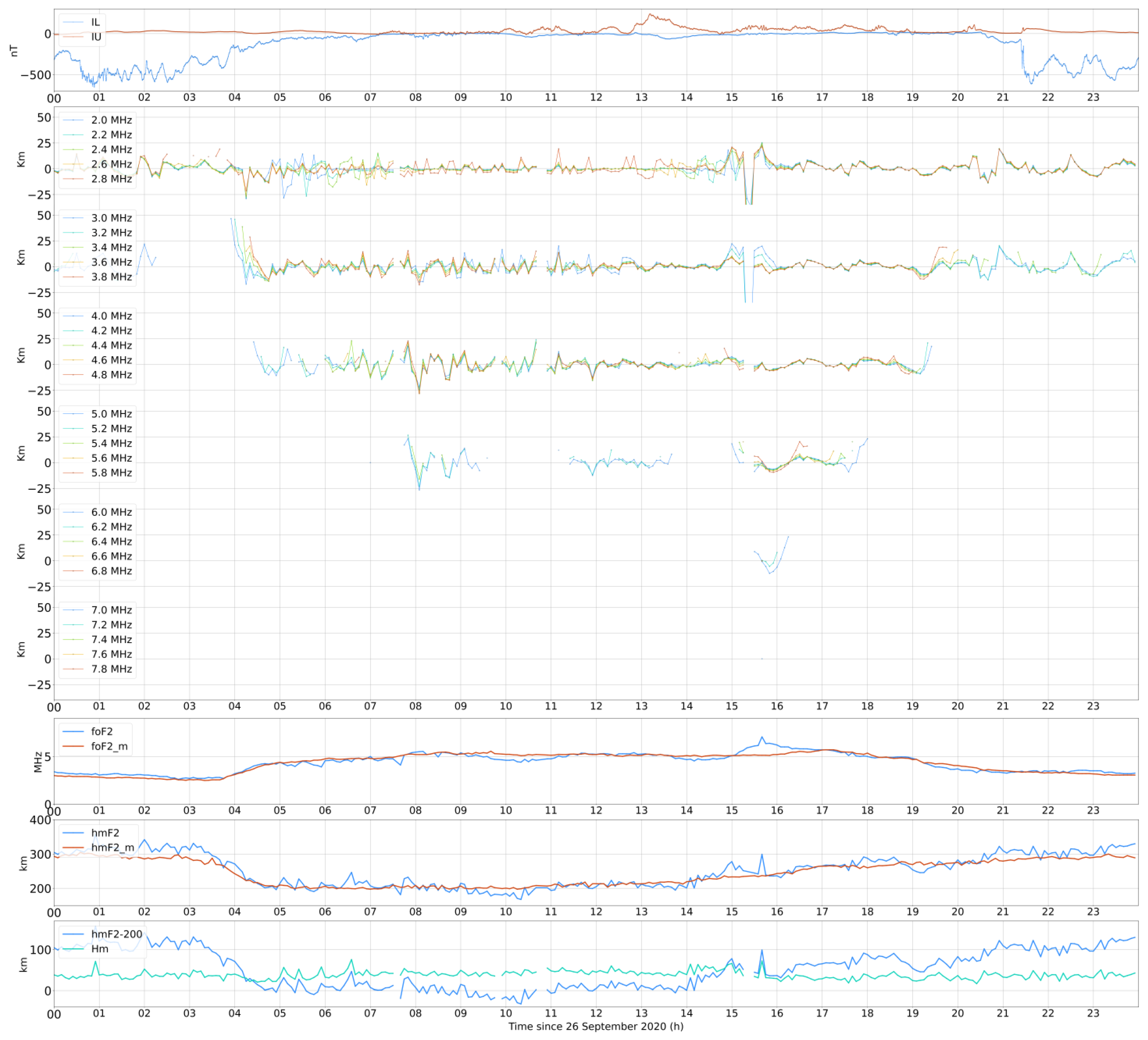
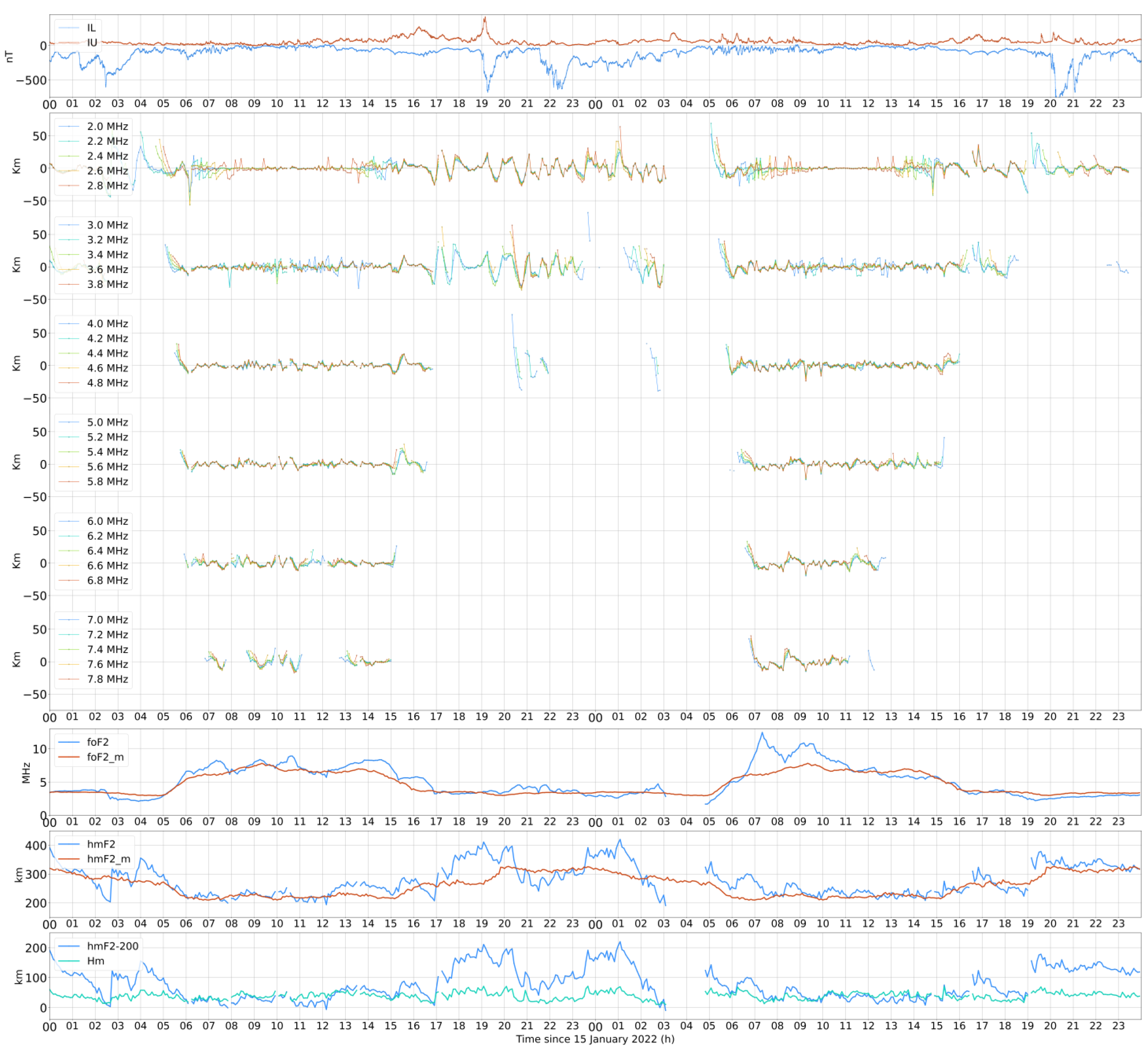
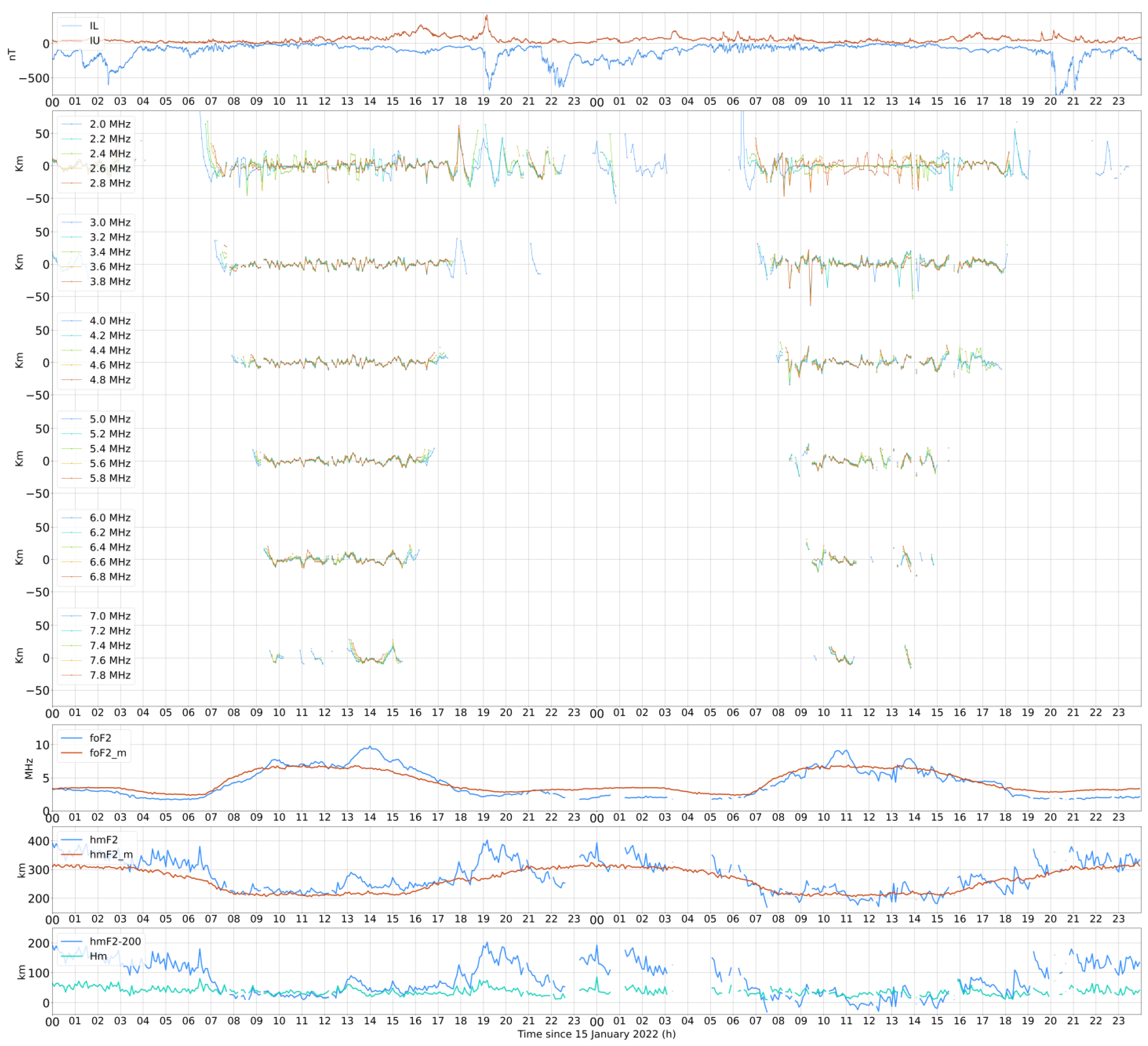
  • The first one is early in the morning, from 0300 to 0400 UT, where the perturbation in the iso-ionic heights is seen at lower frequencies (2.0–2.8 MHz); at the same time, a sudden increase in height and in the scale height is observed. A sharp decrease is observed in foF2 which lasts for one hour before it starts to increase again. A sudden upward jump in the height of the F-region ionization peak (hmF2) is followed by a quick descent of the hmF2, while the density of the F peak (NmF2) increases as the hmF2 moves down. This sequence of events is connected to the equatorial “sunrise undulation” (SU) [30]. Its anecdotal existence has been reported in both Jicamarca, Peru [31,32], and Trivandrum, India [30,33]. It was originally thought [32,33,34] that the SU was due to an electrodynamical effect, analogous to the well-known evening pre-reversal electric field effect [35,36]. This was suggested because of similarities between the electrodynamical conditions prevailing at sunset and sunrise in terms of an electric field reversal which pushes the plasma down in the morning before sunrise and then upward afterwards. Upon closer scrutiny, however, Ambili et al. [30], using a detailed set of digital ionosonde observations at Trivandrum, concluded that the SU actually has a photochemical origin, where vertical transport plays no direct role [37].
  • The second period occurs from 0700 to 1300 UT (0900 to 1500 LT). During this interval, quasi-periodic oscillations are observed at higher frequencies (4.0–7.0 MHz), while at the same time, there is an uplift of the F2 layer and an increase in the peak density (foF2). The scale height shows the same oscillatory behavior as the (hmF2-200) parameter [38]. The IU and IL indicators represent magnetic field perturbations induced by local auroral electrojet activity, which generates enhanced thermospheric heating and wind that are coupled with the ionosphere and propagate south-east as gravity waves. In this scenario, the sharp enhancement of both westward (IL) and eastward (IU) electrojet indices recorded at 0800 UT triggered waves assumed to travel with a speed of 500–1000 m/s (e.g., [39]), which should reach Athens (a distance of about 3000 km) in 1.0–1.5 h. This is, indeed, the time when the main oscillation in ionospheric plasma was observed (see the observed ionospheric disturbances in the time interval 1030–1300 UT).
Another indicative day to examine as a case study is 26 September 2020. The height iso-density data and the critical ionospheric characteristics for this day are shown in Figure 3 in the same manner as in Figure 2. The most pronounced perturbation is observed between 1500 and 1600 UT. Although this is too sharp, that could be regarded as an outlier, the ionograms show that this perturbation was due to a sudden uplift of the F2 layer. The sharp intensification detected at 1300–1330 UT in both electrojets (see IL and IU indices), was expected to activate disturbances that would reach Athens 1–1.5 h later, assuming again a south-west propagation moving at 500–1000 m/s as before. Therefore, it matches fairly well with the observed sharp perturbation in the middle latitude ionosphere over Athens.
At this point we have to comment on the relation between the scale height, Hm, and the peak height hmF2. As reported by McNamara et al. [38], during periods of TIDs, the oscillations in the reduced height hmF2-200 and in Hm are concurrent. This is a requirement in order for the recombination rate within the specific oscillating layer and hence, the plasma density, to be modified according to altitude change due to LSTIDs. Here we consider again the relative variability of the two characteristics in Figure 2 and Figure 3. Only during specific time intervals the two characteristics varied closely in magnitude. This was observed on 24 September 2020, from 0300 UT to 0400 UT and from 0800 UT to 1200 UT. On 26 September 2020, it was observed from 0500 UT to 0700 UT and from 1400 UT to 1600 UT. During these time intervals, LSTID activity was likely; however, additional criteria have to be satisfied in order to be more confident in that. This will be analyzed in the next section.

3.2. A Methodology for LSTID Identification
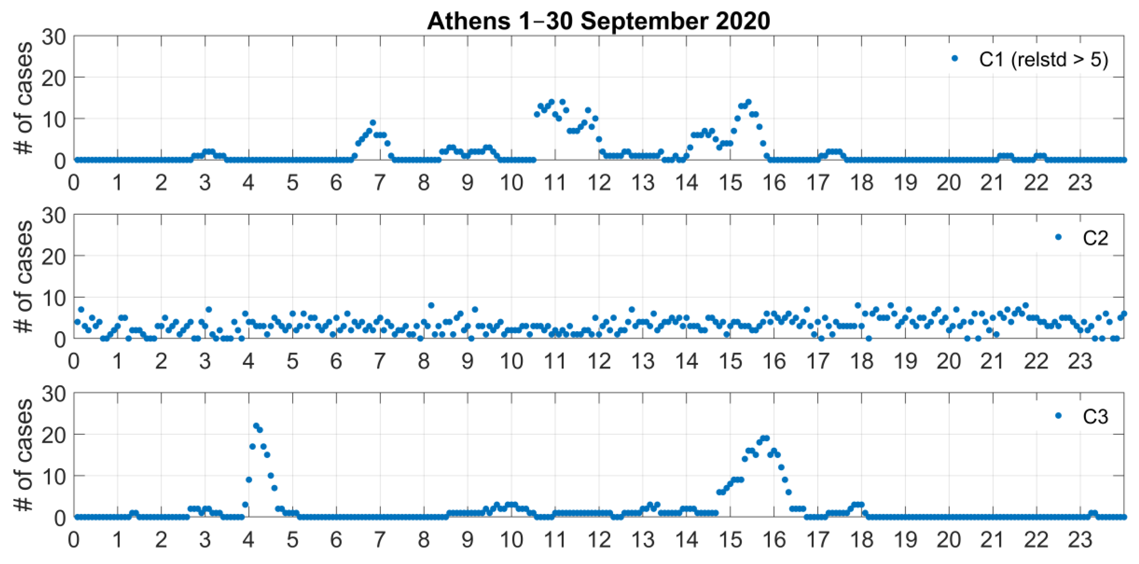
Based on the evidence provided in the previous section, simultaneous fulfillment of three conditions is considered as a key requirement for the identification of LSTID activity at the local scale: the significant variability of the foF2 critical frequency; the relative displacement of the F2 layer up-wards; and the concurrent variation of the scale height with the hmF2 peak electron density height. Hence, we propose the following criteria to be used for the identification of LSTIDs:
C1.
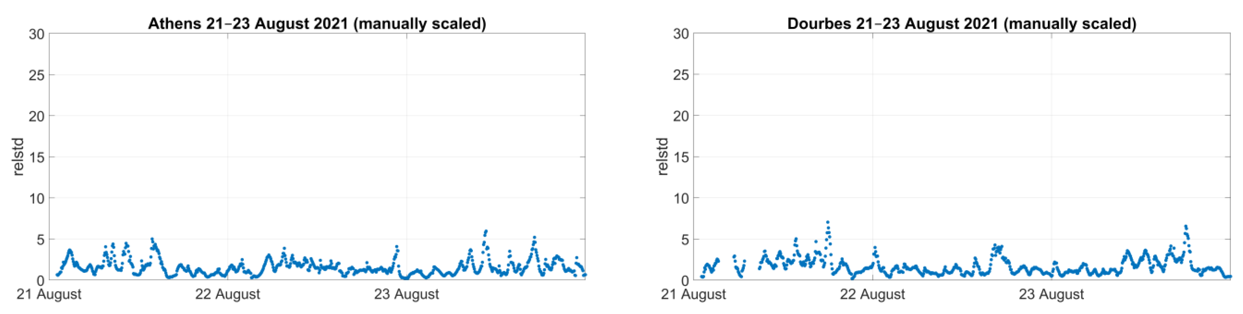
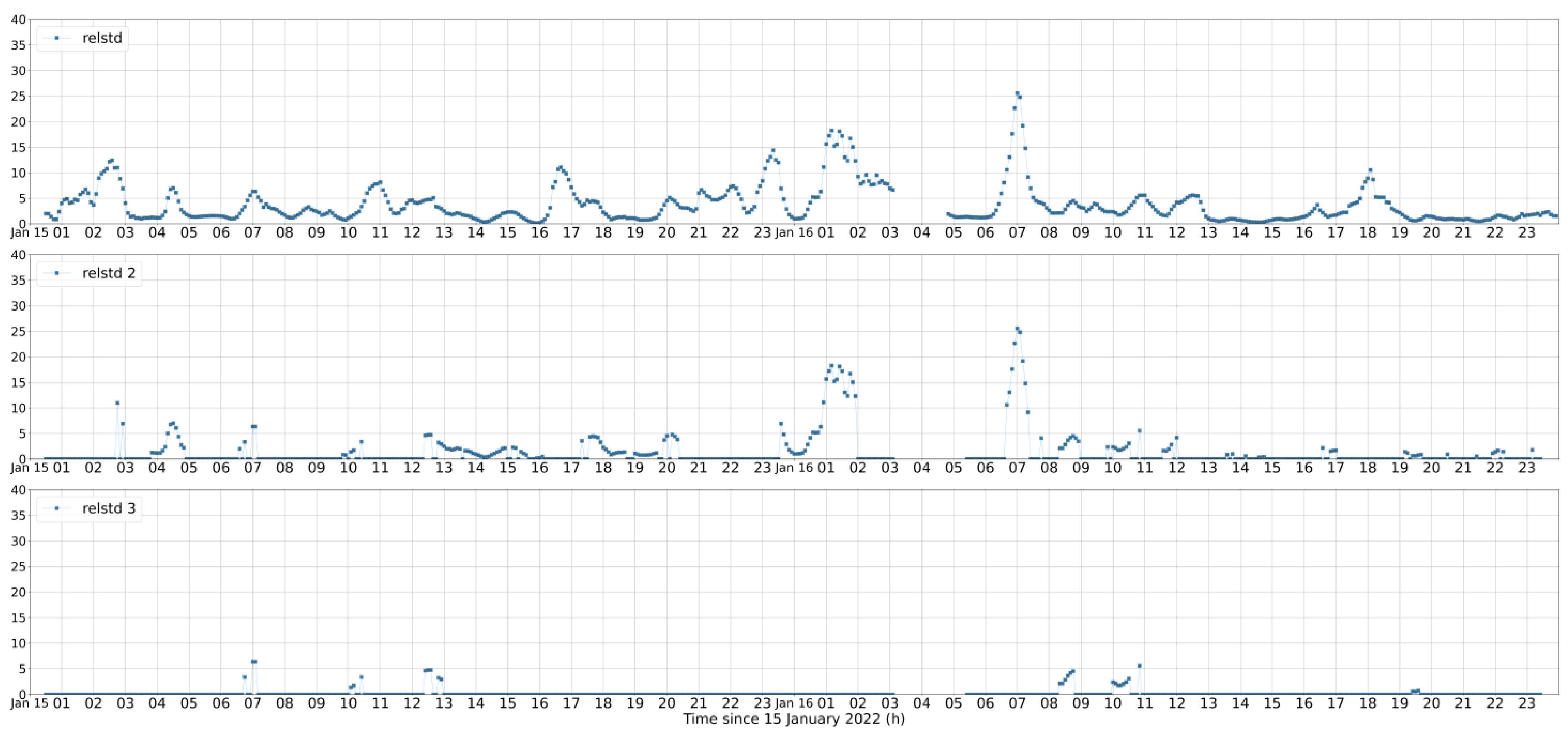
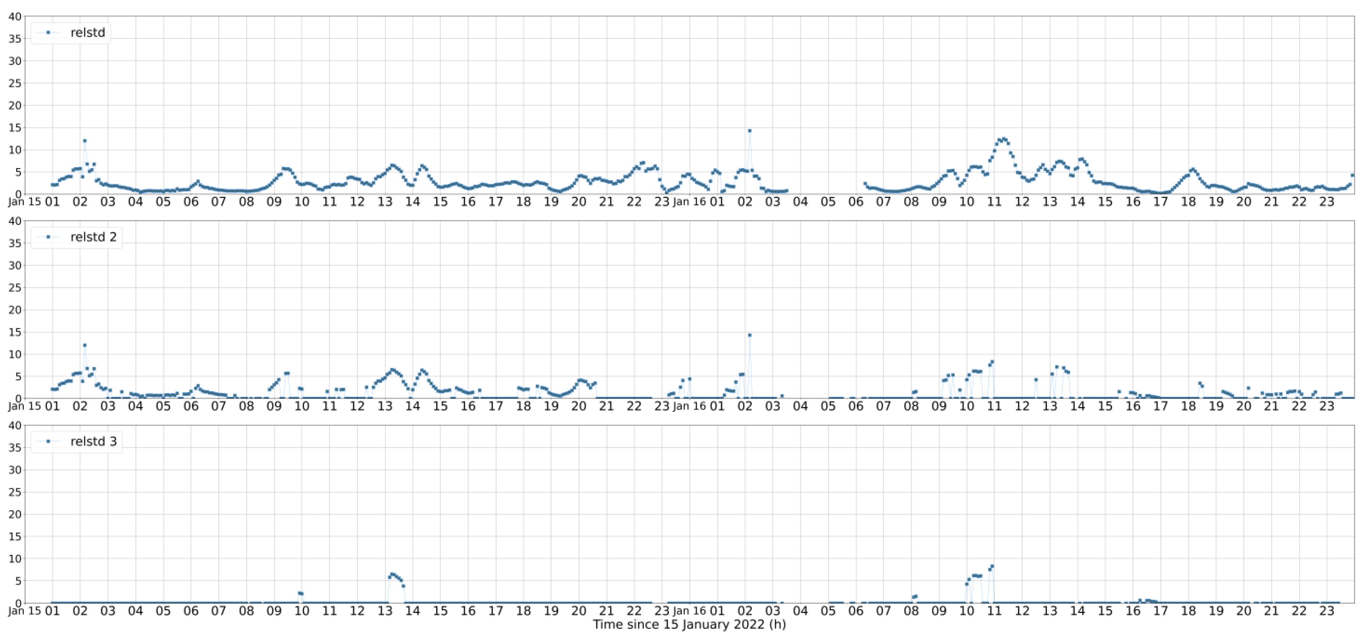
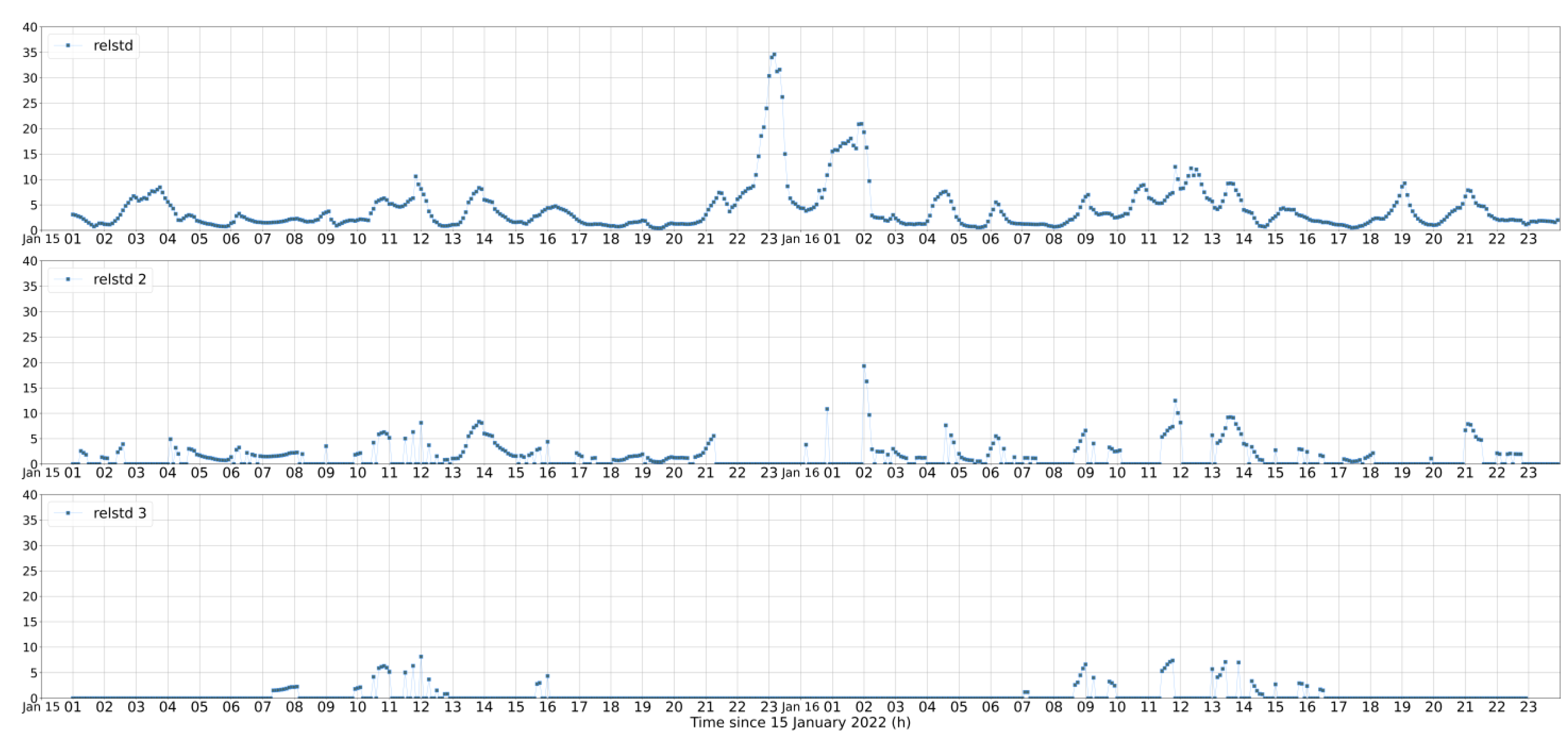
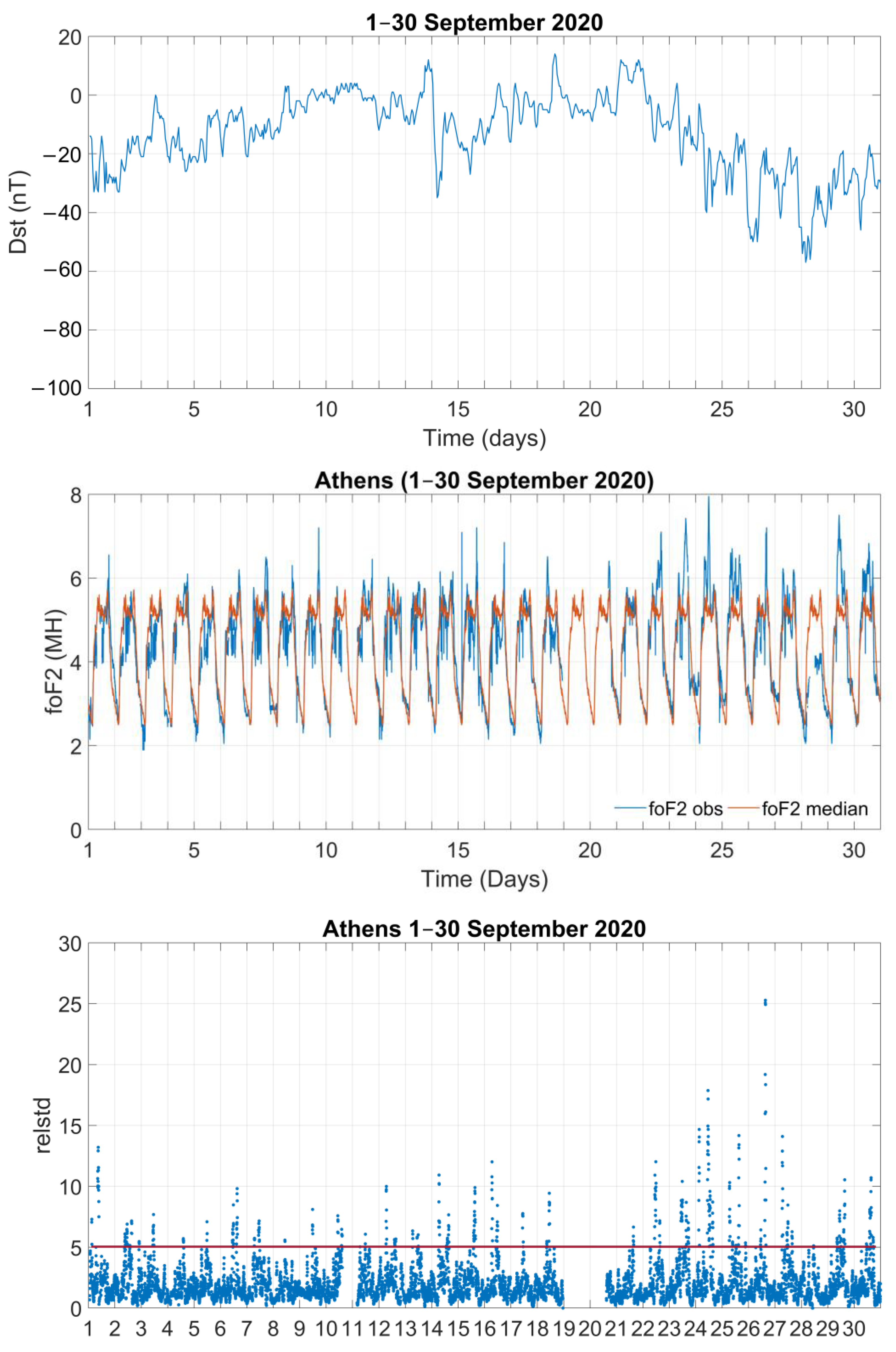
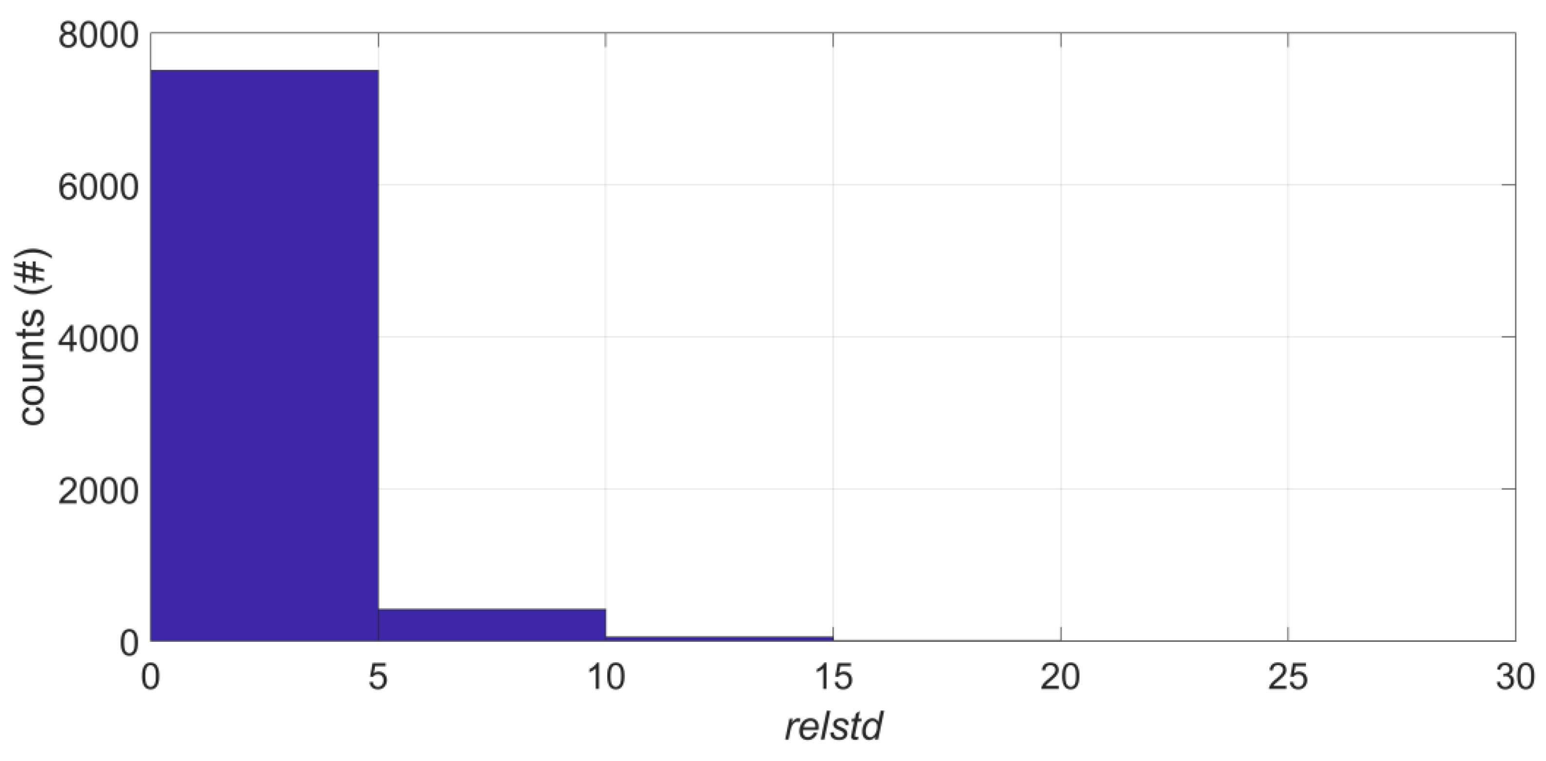
The cut-off frequency foF2 must be highly variable. We propose to quantify the variability based on the relative standard deviation of the foF2, according to the formula:
relstd = std_foF2/std_foF2median,
where std_foF2 is the standard deviation of the foF2 actual observations within 1 h. In the following analysis, the std estimates for each time stamp were based on the records obtained centered around this time stamp (i.e., half an hour before and after the time stamp). std_foF2median is the standard deviation of the foF2 medians within (the same as in std_foF2) 1 h.
Following its definition, relstd values greater than 1 are considered important for the designed purposes, since they are indicative of the increased variability of the foF2 critical frequency.
C2.
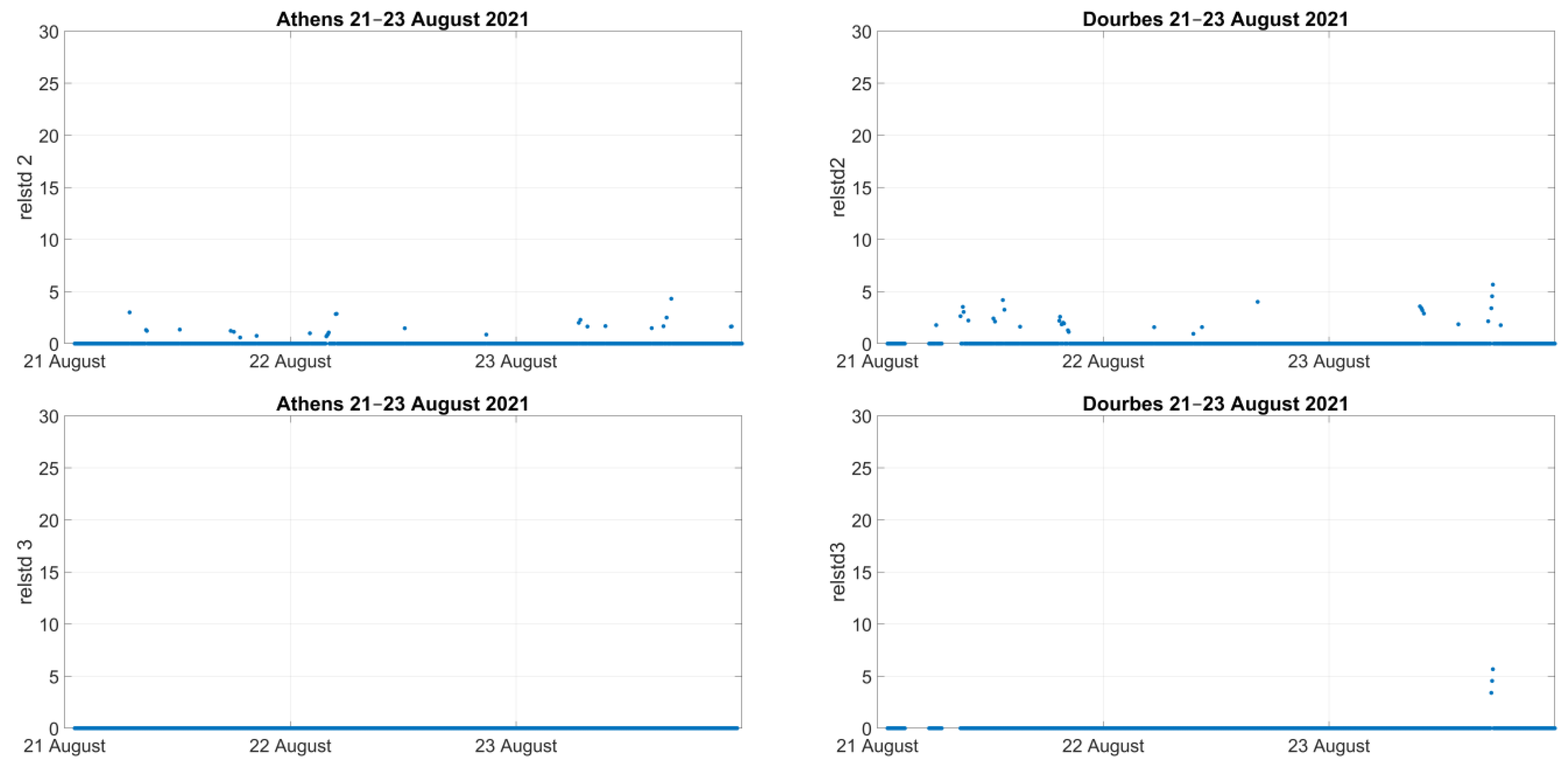
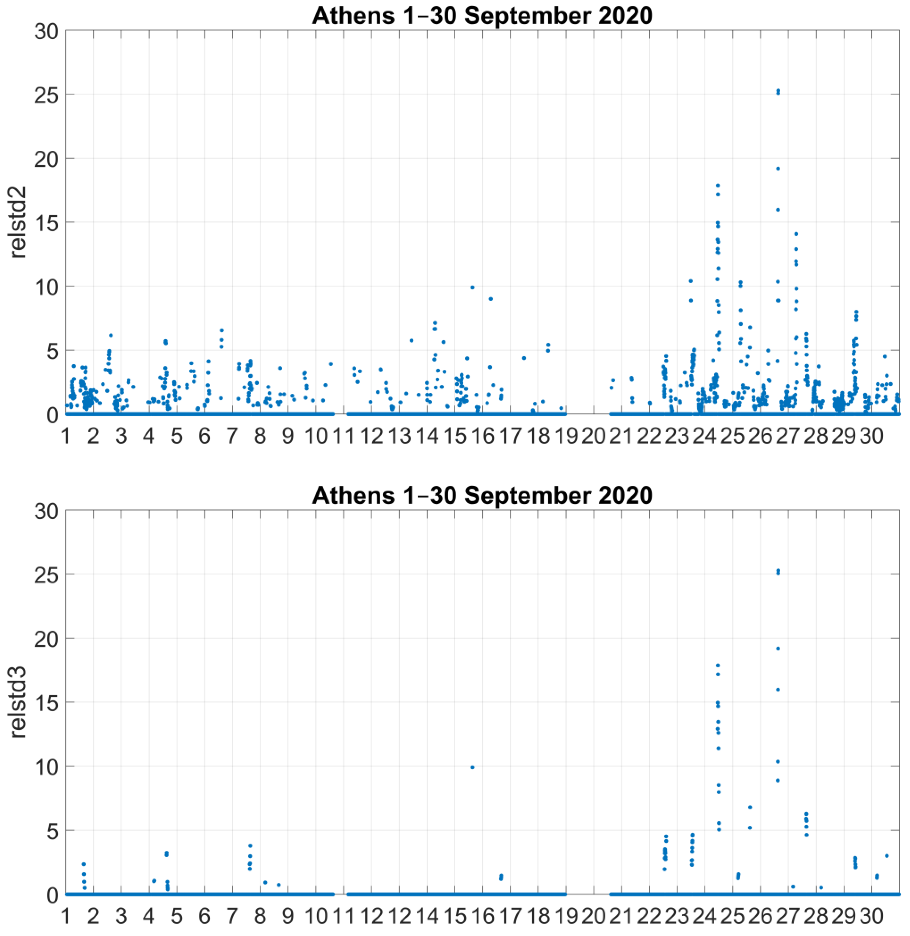
The uplift of the F2 layer, seen as an increase in the hmF2. Here, the increase in the hmF2 is considered significant when the relative positive deviation of the hmF2 observed value from the monthly median (i.e., dhmF2 (%) = ((hmF2obs–hmF2median)/hmF2median) × 100) is greater than the relative standard deviation of the hmF2 values taken into account for the estimation of the median (i.e., (STDmedian/hmF2median) × 100) at the same location and time of the day. As a result of this comparison, we assigned 1 to cases characterized by an increase in hmF2 and 0 to the rest, to be multiplied with the relstd values received above. Therefore, the resulted relstd2 values become zero in case of no hmF2 increase, while they are equal to the relstd in the opposite case.
C3.
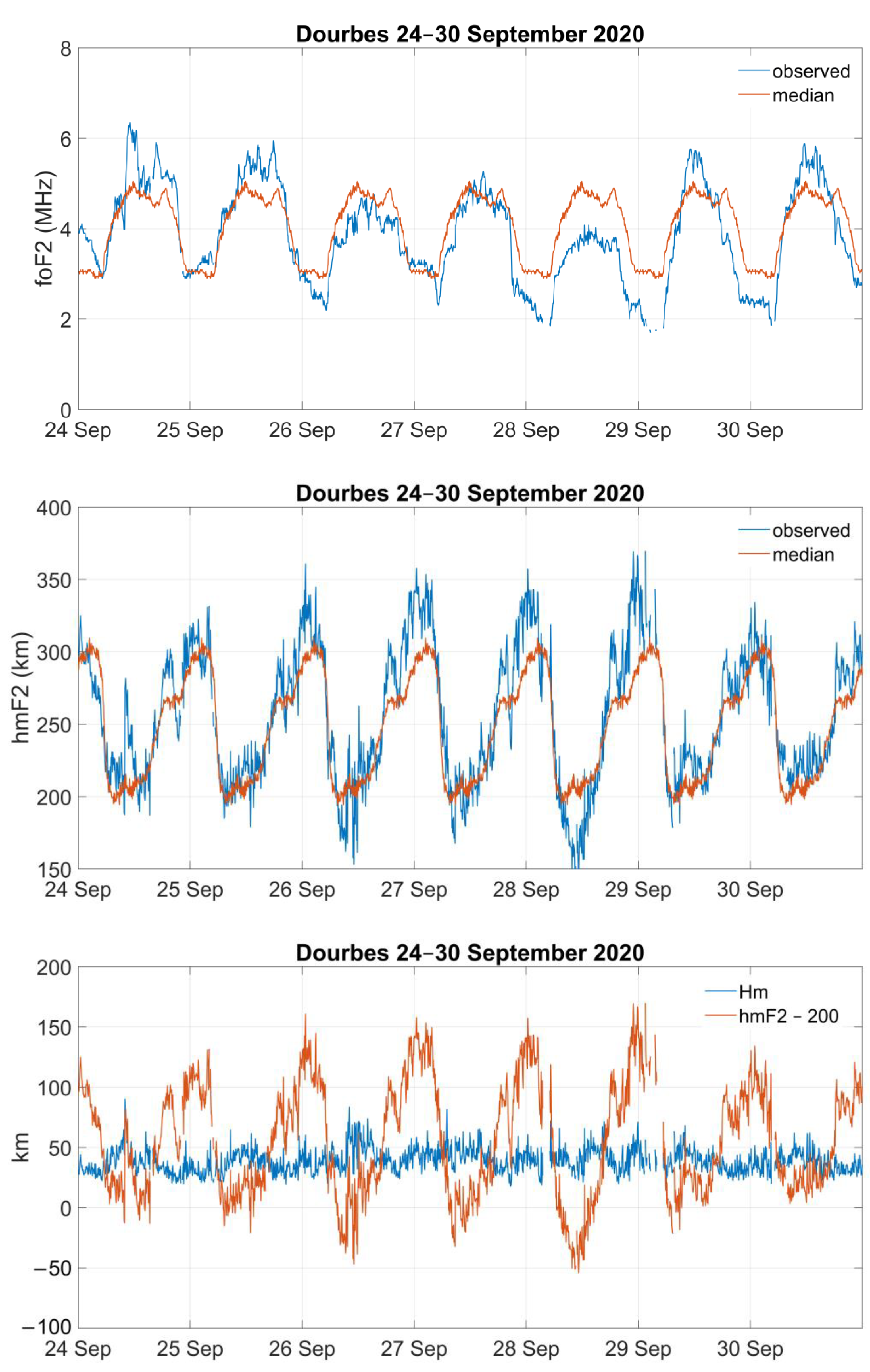
The concurrent variation of (hmF2-200) and the effective scale height, Hm. This is identified using the Kolmogorov–Smirnov (KS) test. The test is applied on two series/vectors of (scalar) data x1 and x2 and returns a test decision for the null hypothesis that the data in vectors x1 and x2 are from the same continuous distribution, for a prespecified significance level. In the present study, the kstest2 MATLAB function, which implements the KS test, was adopted. The alternative hypothesis is that x1 and x2 are from different continuous distributions. The result h is 1 if the test rejects the null hypothesis and 0 otherwise. The adopted significance level in this study is 5%. The KS was applied over (hmF2-200) data (x1) and scale F2 data (x2). Following the implementation of the C3 criterion, the resultant relstd3 values maintained relstd2 ones in case they were accompanied by the concurrent variation of (hmF2-200) and the effective scale height, while returning zeros otherwise.
In the following sections, the performance of the proposed methodology was tested during:
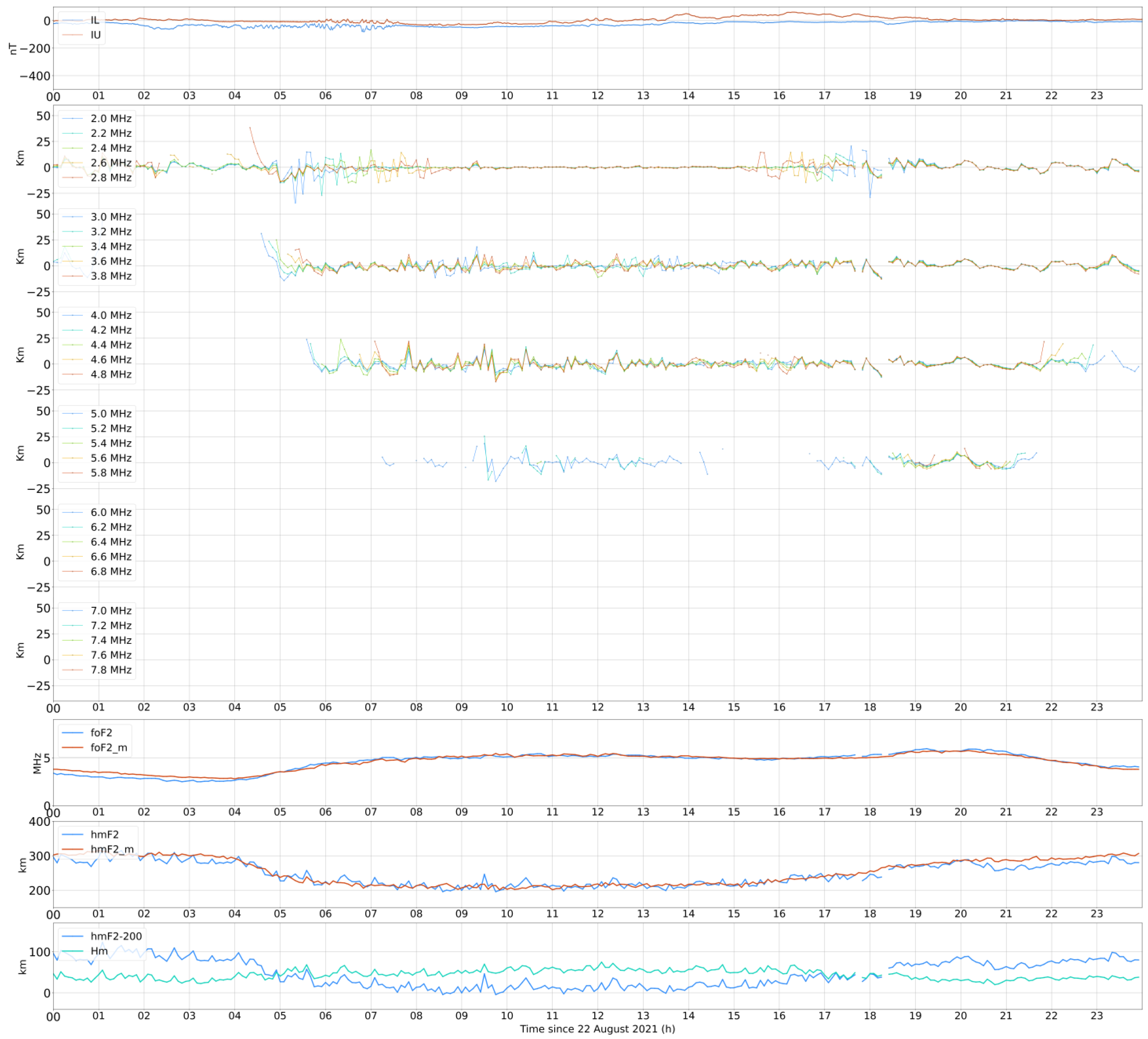
  • A quiet interval where no geomagnetic or lower atmosphere forcing had occurred (21–23 August 2021).
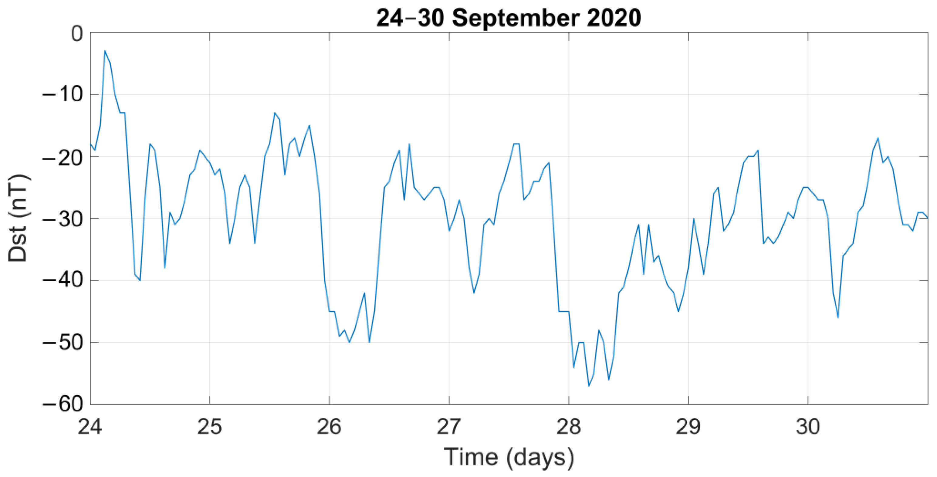
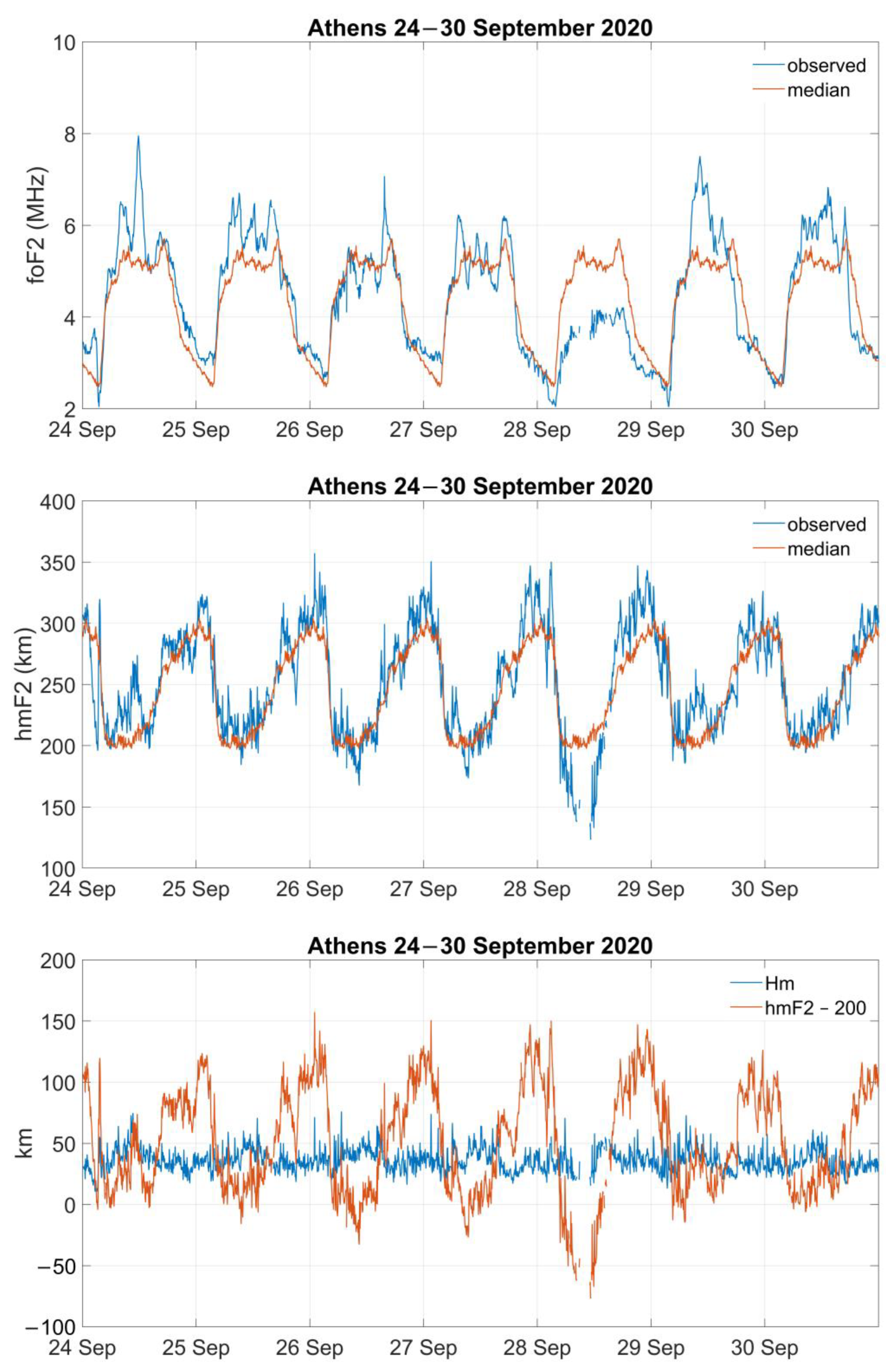
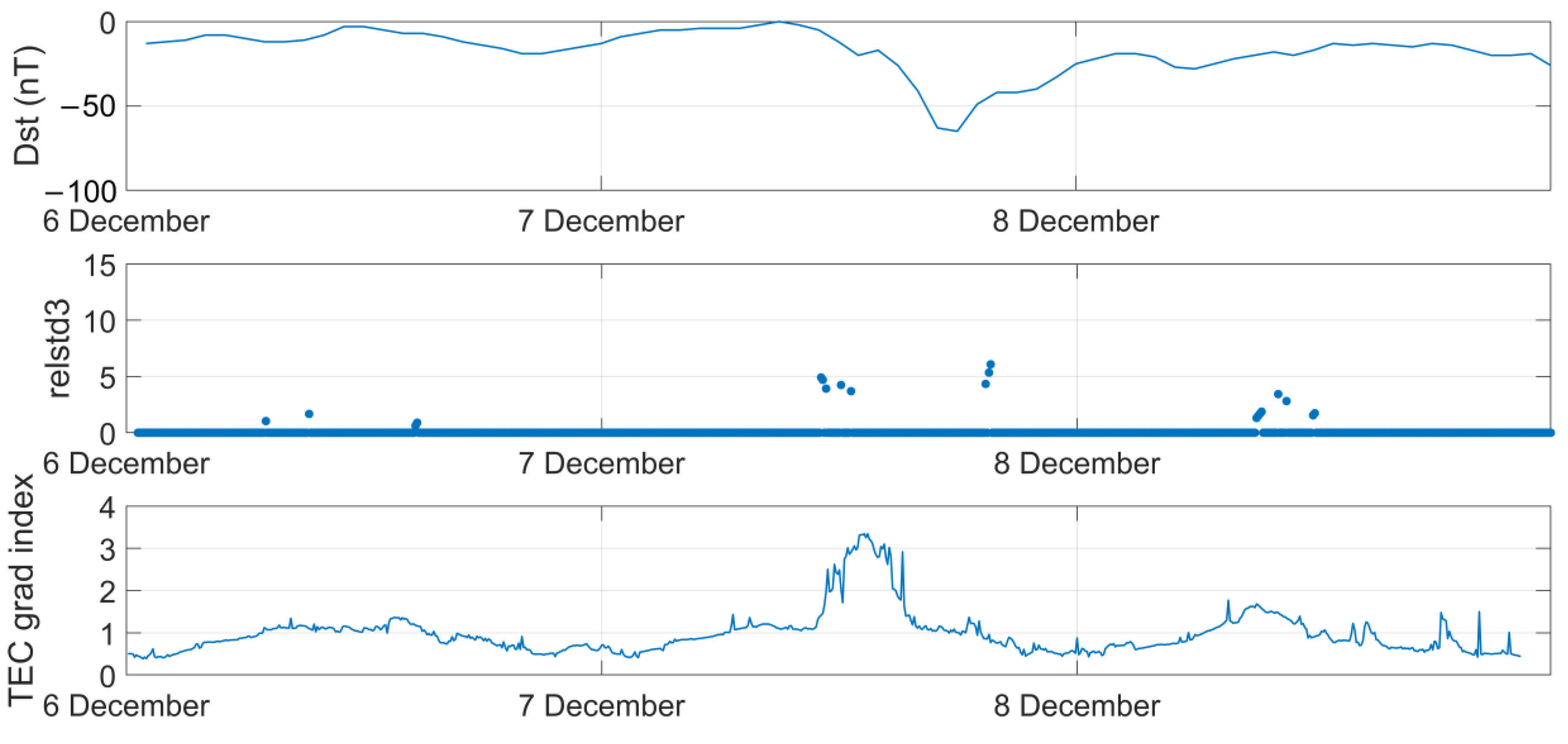
  • Two disturbed intervals with moderate geomagnetic activity (24–29 September 2020 and 6–8 December 2022).
  • A disturbed interval with lower atmosphere forcing (15–16 January 2022).
  • A whole month (September 2020) covering a wider range of geomagnetic activity conditions.

3.3. Evaluation of the LSTID Identification Methodology

3.3.1. Quiet Period

The period of 21–23 August 2021 was selected as an indicative quiet period, because it was one of the few cases with no auroral activity for three consecutive days. The ionospheric response in terms of the height iso-density data and the critical ionospheric characteristics foF2, hmF2, and Hm (manually scaled values) over the stations of Athens and Dourbes on 22 August 2022 is presented in Figure 4 and Figure 5, respectively. For visualization purposes we show here the observations obtained only on this one day. However, the evidence is similar on all days of this geomagnetically quiet time interval.
Despite the fact that during this period, geomagnetic and magnetospheric conditions were very quiet, the height iso-density data show some oscillatory-like disturbances at dawn and dusk hours, especially at the lower frequencies. These disturbances were more evident over Athens in the dusk sector, where they were observed in all frequency ranges. However, the critical ionospheric characteristics foF2 and hmF2 for this day did not share the same oscillatory behavior. In addition, the F2 layer was not uplifted above the monthly median levels. The ionograms (not shown here) indicate MSTID activity, which might have been due to the lower atmosphere forcing or local atmosphere conditions, including the solar terminator crossing, and this may be considered as the cause of the oscillations at the height of the ionospheric plasma.
The application of the set of criteria for the definition of LSTID occurrence is presented in Figure 6 for both Athens and Dourbes. In the first row, we present the relstd values for both stations. It is important to underline that there is no daily pattern and that the relstd parameter shows small variations throughout the whole interval, with no pronounced peaks, remaining in general below the value of 5. In the plots shown in the second row, we applied the filter to relstd values, considering criterion C2 which concerns the condition for positive hmF2 variation. The resultant relstd2 becomes zero in case of no hmF2 increase, while it keeps relstd values in the opposite case. Finally, in the plots shown in the third row, we applied the last filter according to the criterion C3, which takes into account the results of the KS test. In this third step, the relstd3 values becomes zero when C3 is not satisfied, while it keeps the relstd2 values in the opposite case. The combined results (i.e., C1 AND C2 AND C3) indicate no LSTD activity for this time interval in both locations, as relstd3 is mainly zero (with a weak exception observed in Dourbes only in the afternoon hours of August 23).

3.3.2. Geomagnetic Storm Conditions

As a next step, we applied the criteria for the determination of LSTID to the data received in the time interval of 24–30 September 2020 in the Athens and Dourbes Digisonde stations. The ionospheric response over Athens for this time interval is presented in Figure 1, while for the Dourbes location, it is presented in Figure 7 to demonstrate that, again, the most pronounced oscillations in foF2 were observed on the day 24 September 2020.
The results obtained from the application of the proposed criteria are presented in Figure 8 for Athens and Dourbes, in the same manner as in Figure 6. Concerning the variation of the relstd over Athens (see the plots in the top row), the peaks around 1130 UT (24 September 2020) and 1530 UT (26 September 2020) are among the most pronounced ones, but there are also several additional peaks present in almost all the days. In the plots shown in the second row, we applied the additional filter, considering criterion C2, while the results shown in the third row were formulated by the final filter according to the criterion C3. The combined result from all three criteria returns two main peaks: one around 1130 UT on 24 September 2020 with a duration of ~70 min, and one around 1530 UT on 26 September 2020 with a duration of ~20 min, which are the ones corresponding to LSTID conditions according to the physical interpretation presented above (see Section 3.1).
It may also be important to assess the results received on 28 September 2020. During this day, large-scale negative ionospheric storm effects were observed in Athens (see Figure 1). Given that the amplitude of TIDs is directly proportional to the background electron density [1], negative storm conditions are not favorable for the detection of LSTIDs due to the low electron density. Although the relative standard deviation of the foF2 shows some peaks, and all are accompanied by short F2 layer uplifts, the KS tests did not encounter any significant variation between (hmF2-200) and Hm. As a result, not all three criteria proposed in the LSTID identification methodology were met simultaneously, and their combined effect shows the absence of LSTID activity, as expected from the ionization conditions. Two other interesting cases concern the days of 29 and 30 September 2020, that are characterized by significant positive storm effects. Based on their morphology, these are better attributed to large-scale thermospheric changes [39,40]. Potential LSTID activity was mainly observed at daytime hours during both days, with quasi-oscillations in the foF2, which are often accompanied by the uplifting of the F2 layer. This is also reflected in the peaks appearing in the relstd values (top panel in Figure 8), some of which pass also the C2 filter for the condition for hmF2 increase. However, the final filter for criterion C3, which concerns the results of the KS test, eliminates most of the peaks, and finally, only a weak peak around 0930 UT on 29 September 2020 (duration ~30 min) survives, corresponding to LSTID conditions according to the physical interpretation presented above.
The application of the proposed methodology to the Dourbes Digisonde observations indicated significant LSTID activity only on 24 September 2020, which is in agreement with the wave-like foF2 variation. Actually, as it is shown in Figure 7, only during that day, from 1000 UT to 1800 UT, did the foF2 parameter exhibit strong fluctuations, and at the same time, the F2 was uplifted and the scale height Hm varied concurrently with the reduced height hmF2-200. The main peak of relstd3 values was determined at around 1015 UT, with a duration of 45 min. This was slightly earlier than the peak determined in Athens during this day (i.e., on 1130 UT), a time difference that it is consistent with the time delay of LSTIDs’ travelling time from high to middle latitudes in the south-east direction (see also the discussion in Section 3.1).

3.3.3. Lower Atmosphere Forcing: The Case of the Tonga Volcano Eruption

Two different physical mechanisms can cause TIDs to appear after a volcanic eruption: disturbances can be produced directly in the ionosphere at the location of the eruption and travel radially outwards at ionospheric altitudes, or ionospheric disturbances can result from the propagation of various types of waves through the lower atmosphere. The waves propagating through the lower atmosphere are further differentiated into acoustic waves, gravity waves, and Lamb waves, depending on their frequency compared to the acoustic cutoff frequency [41,42]. A volcanic eruption can produce waves of all these types, which will propagate outward from the eruption with different velocities and to different distances before dissipating.
On 15 January 2022, at 0415 UT, the Hunga volcano in Tonga (20.54° S, 175.38° E) [43,44] produced a powerful eruption [45]. For this event, a Lamb wave was detected as the leading wavefront, followed by various disturbances of different natures [46,47,48,49]. Disturbances in the ionosphere over Europe, close to the antipode of the eruption, were identified by Verhulst et al. [27]. LSTIDs propagating through the ionosphere from the site of the eruption are not expected to proceed for such distances [28,42]. Themens et al. [50] indeed find that large-scale TIDs produced directly in the thermosphere above the eruption dissipated after a few thousand kilometers. However, medium-scale TIDs travelling with the Lamb wave front seem to propagate further [50,51], and clear signatures of waves travelling around the globe in the lower atmosphere have been detected [46,52,53]. Waves in the ionosphere over Europe indicative of MSTID activity appeared either at the same time as the ground-level pressure disturbances, for the Lamb waves, or with maximum usable frequency (MUF) delay for disturbances propagating upwards from the troposphere [27].
For this event, the methodology proposed for the identification of LSTIDs was applied to the Digisonde data recorded in three European locations—Athens, Dourbes, and Ebre, to extensively test the efficiency of the proposed considerations in these conditions. These are considered to be extremely challenging, since the volcano eruption took place during the recovery phase of a geomagnetic storm. The Dst index reached a minimum of −91 nT on 14 January at 2300 UT. The ionospheric response in Athens, Dourbes, and Ebre is given in Figure 9, Figure 10 and Figure 11, respectively. The results in Figure 9 show some wave activity over Athens that is evident in the foF2 and hmF2 characteristics during both days. However, there were noticeable differences between the wave activity recorded during daytime and nighttime hours. In the first case, the oscillations tended to occur in higher frequencies and be most pronounced in the foF2 variation, following excursions in the magnetospheric activity. In addition, they were often accompanied by increases in the hmF2, while the scale height (Hm) and the (hmF2-200) parameter varied concurrently on several occasions. However, the situation was different during the night, when the wave activity was observed at lower frequencies (including the foF2), while they were not always related neither to increases in the hmF2, nor to con-variance between the scale height and the (hmF2-200) parameter. The pattern is the same in all three stations, although clearer in Athens and Ebre (see Figure 9 and Figure 11). The analysis of the same observations by Verhulst et al. [27] attributed the nighttime ionospheric response to MSTID activity triggered by lower atmosphere forcing that is not related to geomagnetic activity. Indeed, the proposed criteria are not met simultaneously during the night, and their combined effect practically shows the absence of LSTID activity during nighttime hours in all three locations (see Figure 12, Figure 13 and Figure 14). However, the results indicate weak LSTID activity around noon on 15 and 16 January 2022 in all locations, which is reasonably considered to be the result of the accumulated energy concurrently released in the auroral oval at the longitudes of Norway.
The analysis of this event provides evidence that the methodology proposed here has the capability to separate LSTIDs from MSTIDs. When TIDs are driven by auroral activity, the combined use of the three criteria indicates the existence of LSTID activity (during daytime hours, even though weak in this case). During the nighttime hours, when according to the literature MSTIDs occur, the combined use of the LSTID identification criteria results to no activity at all.

4. Discussion

As already mentioned, LSTIDs are expected to be associated with auroral and geomagnetic activity [1,8,9,10,11]. In this context, one of the key features of the proposed methodology’s capabilities is the reflection of this relationship in the identified disturbances. The evidence provided in the above sections supports the connection, as the LSTID activity tends to follow excursions in auroral electrojets’ activity, expressed here by the IU and IL indicators. In addition, LSTID activity was mainly identified during geomagnetically disturbed days (e.g., the time interval 24—30 September 2020). To further investigate this particular feature of the proposed methodology’s efficiency, the set of the proposed criteria was also applied to the data obtained in Athens for the whole month of September 2020. The variation of the Dst index, together with the ionospheric conditions in terms of the observed and median foF2 and the relstd results, are presented in Figure 15. As the main finding of this analysis, the combined effect of the proposed criteria (bottom panel) shows that the identified LSTID activity clearly tends to follow the geomagnetic activity. Indeed, the relstd3 values were significantly higher in the last days of the month, when the geomagnetic activity level was higher and the ionospheric storm disturbances over Athens were also more intense (see second panel of Figure 15). At this point, it is also very important to stress that the identified activity did not reflect large scale ionospheric storm effects (see for instance the results received on 28–30 September 2020). Neither negative storm conditions nor large-scale ionization increases, rather attributed to large-scale thermospheric changes [39,40], were captured in the obtained results, further supporting the efficiency of the proposed methodology in detecting only the effects of LSTID activity, as it is designed to do.
An additional finding that results from the inspection of Figure 15 is that the more intense spikes of relstd tended to be related with values greater than 5. This is also in agreement with the results obtained during the time interval of 21–23 August 2021 that is representative of quiet conditions in the above analysis. Figure 16 provides the distribution of the relstd values obtained during September 2020 to demonstrate that most of them lie between 0–5, and most probably correspond to quiet (no LSTID activity) conditions. Based on this discussion one may argue that it may serve as a preliminary consideration thresholding of significant LSTID activity. The criterion relstd greater than 5 was partially used in the analysis below.
The efficiency of the proposed methodology is critically based on the validity of all three elements/criteria. In the following, we investigate the relative role of each criterion in the overall performance. In Figure 17, we present the number of cases, summed over September 2020, in which each criterion is met in each hour of day (in UT). Based on this evidence:
i.
The relstd exhibited several peaks during daytime hours and, especially, in the afternoon sector. This is consistent with the appearance of TID effects in the foF2 as they are described by widely accepted phenomenological scenarios [39,40] and compatible with the tendency of LSTID detection during daytime hours when the electron density is higher. There were also two secondary peaks, around 0300 and 1700 UT, that may be related to diurnal variations, as, for instance, sunrise and sunset variability caused by the passage of the solar terminator (sunrise and sunset time in Athens was about 0700–0800 and 1900–2000 local time, respectively).
ii.
No particular diurnal trend was identified concerning the increase in hmF2. This is also consistent with expected features of the LSTID activity. Phenomenological descriptions, as well as physics-based modeling of LSTID generation and propagation, show dominant enhancement of “equatorward wind” and associated upward motion of the ionosphere in midlatitudes during LSTID passage [39,54]. The rise of the F layer has also been confirmed by observations [55]. While the LSTID effects in the foF2 depend strongly on electron density conditions, being non or hardly detectable during low density conditions (e.g., during night or under ionization depletion events), the hmF2 increases are “visible” in all cases [39] (see for instance relevant results during the nighttime hours on 28 September in Figure 1 and Figure 7).
iii.
The concurrent variance between scale height at F2 layer peak and (hmF2–200) shows two clear peaks around 0400 and 1600 UT that roughly coincide with sunrise and sunset times in Athens. Noticeable related activity was also observed in the afternoon hours.
Based on the above discussion, it is clear that none of the three criteria alone can reliably support the identification of LSTID activity, due either to diurnal dependence (e.g., in foF2 and scale height at the F2 layer peak) or to no particular trends (e.g., hmF2). Instead, their combined use provides more reliable identification of the LSTID signatures, also reflecting the vertical structure of the LSTIDs (see also [54] and references therein).
With regard to the assessment of the proposed method’s performance, it is also important to test the results through cross-comparison with other LSTID activity metrics. However, this is a challenging task due to two main reasons: (i) although there are several methods that have been proposed for the identification of LSTIDs in the literature, it is hard to find/obtain results that coincide with the time and space of analysis; and (ii) different methods may differ fundamentally in development and implementation, so that the direct comparison of their results is not straightforward. To meet the challenge, we implemented the proposed methodology in the Dourbes location (a middle-to-high latitude station) in the time interval 6–8 December 2022, which was characterized by moderate storm activity (min Dst = −65 nT). The Dst records and the relstd3 values for this time interval are given in Figure 18 (top and middle panels, respectively). In the bottom panel of Figure 18, we present for comparison purposes the results obtained by the GNSS TEC gradient method that has been proposed by Borries et al. [56]. The method calculates temporal and spatial TEC gradients based on TEC maps. TEC gradients are not a direct signature of TIDs. Therefore, TID occurrence cannot be directly inferred from TEC gradients. Instead, TEC gradients are considered to be precursors of LSTID activity. Significant TEC gradients at high latitudes are indicative of strong ionosphere–thermosphere perturbations, which are in turn considered to be sources of LSTIDs. Such TEC gradients are typically observed in the auroral oval. The method has been recently implemented operationally to complement TechTIDE services, based on the exploitation of European TEC maps [57]. Since the generation of TEC maps averages out steep TEC gradients, rather low thresholds must be assumed for the indication of the probability of LSTID generation. The statistical analysis of TEC gradients shows that the average TEC gradient has an amplitude of about 0.2 mm/km. Alert thresholds can be based on the 90%, 95%, and 99% quantile, derived from the complementary of the cumulative distribution function of the high-latitude region. TEC gradients are considered low with amplitudes below 1.2 mm/km, moderate with amplitudes between 1.2 mm/km and 2 mm/km, and strong above 2 mm/km. The evidence in Figure 18 shows that there is a general agreement between the findings of the two methods, as LSTID activity expressed by relstd3 values tended to follow intensifications in the TEC gradient index. However, it has to be noted that one should not expect a one-to-one relation in the identified peaks, since the GNSS TEC gradient method “predicts” the sources of LSTIDs at high latitudes (“regional” predictions over Europe), while the method proposed here identifies the LSTID activity in one single location (specifically, over Dourbes).

5. Concluding Remarks and Future Work

In this paper, a new methodology for the identification of LSTID activity at the local scale is proposed. It is based on the analysis of ionospheric observations obtained by ground-based mid-latitude ionosondes, namely the foF2 critical frequency, the peak electron density height hmF2, and the scale height at F2 layer peak, Hm. LSTID occurrence is determined upon (a) high foF2 variability, (b) increase in the hmF2, and (c) covariance of the reduced height hmF2-200 and scale height at hmF2.
The efficiency of the proposed methodology was tested in a range of ionospheric conditions, including both quiet and disturbed periods. The results provide evidence for the potentiality of the new methodology in following LSTID activity with the following characteristics for the proposed indicator: (i) it follows enhancements in geomagnetic/magnetospheric activity, with no sensitivity to large-scale increases or decreases in the ionospheric ionization; (ii) it is not sensitive to MSTIDs imposed by lower atmosphere forcing; (iii) it identifies wave-like disturbances that tend to occur in daytime hours, especially in the local afternoon sector. All of the above are fully consistent with LSTID activity features.
The proposed methodology has shown capability in separating LSTIDs from MSTIDs (see the analysis of the Tonga event in Section 3.3.3). Other limitations may concern the effect of electric-field-driven disturbances on the method’s results. Indeed, the method was only tested at individual locations in the middle latitudes during quiet to moderately disturbed geomagnetic conditions, where the contribution of electromagnetic drifts to foF2 and hmF2 variation is generally considered to be less effective (compared to equatorial/low latitudes). Therefore, it is difficult to come to conclusion on any sensitivity of the method’s results to electric-field-related disturbances, which may be significant even in the middle latitude zone during intense storm conditions, e.g., [58]. To this effect, a more detailed investigation is required, based on the implementation of the proposed methodology in a dense network of ionosondes and the analysis of a large number of geomagnetic storms of different levels of intensity using Digisonde data from stations at middle and low/equatorial latitudes.
Apart from the assessment of the method’s performance in more test periods/locations, future work may also include additional efforts for the assessment of the method’s performance through cross-comparison with other TID activity metrics, such as, for instance, the ones provided by TechTIDE methodologies [57] and/or scaling of the proposed LSTID indicator, providing metrics regarding the confidence level of the results. It is also expected that the analysis of results obtained through the implementation of the proposed methodology in a dense network of Digisondes could contribute valuable insight information on LSTID propagation characteristics that would be of interest to both scientific and operational applications. Finally, the proposed methodology could be implemented for real- or near-real-time applications. In such a plan, there is a series of challenges to be addressed, which are mainly associated with the quality of the data that are routinely available (e.g., autoscaling errors or data gaps), but this is also a subject for future work.

Author Contributions

Conceptualization, I.T. and A.B.; methodology, I.T., A.B. and K.K.; software, K.T. and T.H.; validation, I.T., A.B., K.T., K.K. and T.H.; formal analysis, I.T., K.T. and T.H.; investigation, I.T.; resources, I.T.; data curation, I.T., and A.B.; writing—original draft preparation, I.T.; writing—review and editing, I.T., A.B., K.T., K.K. and T.H.; visualization, I.T. and T.H.; supervision, I.T.; project administration, I.T.; funding acquisition, A.B. All authors have read and agreed to the published version of the manuscript.

Funding

This research was funded by the TechTIDE project, Grant Agreement 776011 funded by the Horizon 2020 Programme of the European Commission, and partly supported by the PITHIA-NRF project, Grant Agreement 101007599 funded by the Horizon 2020 Programme of the European Commission, and the T-FORS Project, Grant Agreement 101081835 funded by the Horizon Europe Programme of the European Commission. A. Belehaki acknowledges financial support provided by the AFRL grant award FA9550-19-1-7019.

Institutional Review Board Statement

Not applicable.

Informed Consent Statement

Not applicable.

Data Availability Statement

Digisonde observations were retrieved from the Global Ionosphere Radio Observatory (GIRO) data repository (http://giro.uml.edu/, accessed on 14 January 2023). The auroral electrojet indicators IU and IL were derived from FMI/IMAGE magnetometer chain and are available at https://space.fmi.fi/image/www/index.php?page=home (accessed on 14 December 2022). Records of the Dst index are available by the World Data Center (WDC) for Geomagnetism, Kyoto (http://wdc.kugi.kyoto-u.ac.jp/dstdir/, accessed on 14 January 2023). The GNSS TEC gradient data were retrieved from the TechTIDE API (http://https://techtide-srv-pub.space.noa.gr:8443/api/, accessed on 14 January 2023).

Conflicts of Interest

The authors declare no conflict of interest.

References

  1. Hunsucker, R.D. Atmospheric gravity waves generated in the high-latitude ionosphere: A review. Rev. Geophys. 1982, 20, 293–315. [Google Scholar] [CrossRef]
  2. Hocke, K.; Schlegel, S. A review of atmospheric gravity waves and travelling ionospheric disturbances. Ann. Geophys. 1996, 14, 917. [Google Scholar]
  3. Reinisch, B.; Galkin, I.; Belehaki, A.; Paznukhov, V.; Huang, X.; Altadill, D.; Buresova, D.; Mielich, J.; Verhulst, T.; Stankov, S.; et al. Pilot ionosonde network for identification of traveling ionospheric disturbances. Radio Sci. 2018, 53, 365–378. [Google Scholar] [CrossRef]
  4. Hernández-Pajares, M.; Juan Zornoza, J.M.; Sanz, J. Medium Scale Traveling Disturbances Affecting GPS Measurements: Spatial and Temporal Analysis. J. Geophys. Res. Atmos. 2006, 111, A07S11. [Google Scholar] [CrossRef]
  5. Ross, W. The estimation of the probable accuracy of high frequency radio direction-finding bearings. J. Inst. Electr. Eng.-Part IIIA: Radiocommun. 1947, 94, 722–726. [Google Scholar] [CrossRef]
  6. Pintor, P.; Roldán, R. The impact of the high ionospheric activity in the EGNOS performance. Coordinates Magazine 2015, 11, 20–28. [Google Scholar]
  7. Nickisch, L.J.; Hausman, M.A.; Fridman, S.V. Range rate-Doppler correlation for HF propagation in traveling ionospheric disturbance environments. Radio Sci. 2006, 41, RS5S39. [Google Scholar] [CrossRef]
  8. Tsugawa, T.; Saito, A.; Otsuka, Y. A statistical study of largescale traveling ionospheric disturbances using the GPS network in Japan. J. Geophys. Res. 2004, 109, A06302. [Google Scholar] [CrossRef]
  9. Ding, F.; Wan, W.; Liu, L.; Afraimovich, E.L.; Voeykov, S.V.; Perevalova, N.P. A statistical study of large scale traveling ionospheric disturbances observed by GPS TEC during major magnetic storms over the years 2003–2005. J. Geophys. Res. 2008, 113, A00A01. [Google Scholar] [CrossRef]
  10. Ding, F.; Wan, W.; Ning, B.; Zhao, B.; Li, Q.; Zhang, R.; Xiong, B.; Song, Q. Two dimensional imaging of largescale traveling ionospheric disturbances over China based on GPS data. J. Geophys. Res. 2012, 117, A08318. [Google Scholar] [CrossRef]
  11. Ferreira, A.A.; Borries, C.; Xiong, C.; Borges, R.A.; Mielich, J.; Kouba, D. Identification of potential precursors for the occurrence of Large-Scale Traveling Ionospheric Disturbances in a case study during September 2017. J. Space Weather. Space Clim. 2020, 10, 32. [Google Scholar] [CrossRef]
  12. Chimonas, G.; Hines, C.O. Atmospheric gravity waves launched by auroral currents. Planet. Space Sci. 1970, 18, 565–582. [Google Scholar] [CrossRef]
  13. Deng, Y.; Heelis, R.; Lyons, L.R.; Nishimura, Y.; Gabrielse, C. Impact of low bursts in the auroral zone on the ionosphere and thermosphere. J. Geophys. Res. Space Phys. 2019, 124, 10459–10467. [Google Scholar] [CrossRef]
  14. Hayashi, H.; Nishitani, N.; Ogawa, T.; Otsuka, Y.; Tsugawa, T.; Hosokawa, K.; Saito, A. Large scale traveling ionospheric disturbance observed by superDARN Hokkaido HF radar and GPS networks on 15 December 2006. J. Geophys. Res. 2010, 115, A06309. [Google Scholar] [CrossRef]
  15. Lei, J.; Burns, A.G.; Tsugawa, T.; Wang, W.; Solomon, S.C.; Wiltberger, M. Observations and simulations of quasiperiodic ionospheric oscillations and largescale traveling ionospheric disturbances during the December 2006 geomagnetic storm. J. Geophys. Res. 2008, 113, A06310. [Google Scholar] [CrossRef]
  16. Shiokawa, K.; Otsuka, Y.; Ogawa, T.; Balan, N.; Igarashi, K.; Ridley, A.J.; Knipp, D.; Saito, A.; Yumoto, K. A large scale traveling ionospheric disturbance during the magnetic storm of 15 September 1999. J. Geophys. Res. 2002, 107, 1088. [Google Scholar] [CrossRef]
  17. Ding, F.; Wan, W.; Ning, B.; Wang, M. Large-scale traveling ionospheric disturbances observed by GPS total electron content during the magnetic storm of 29-30 October 2003. J. Geophys. Res. 2007, 112, 309. [Google Scholar] [CrossRef]
  18. Guo, J.; Liu, H.; Feng, X.; Wan, W.; Deng, Y.; Liu, C. Constructive interference of large-scale gravity waves excited by interplanetary shock on 29 October 2003: CHAMP observation. JGR 2014, 119, 6846–6851. [Google Scholar] [CrossRef]
  19. Kotake, N.; Otsuka, Y.; Tsugawa, T.; Ogawa, T.; Saito, A. Climatological study of GPS total electron content variations caused by medium-scale traveling ionospheric disturbances. J. Geophys. Res. 2006, 111, 1–8. [Google Scholar] [CrossRef]
  20. Frissell, N.A.; Baker, J.B.H.; Ruohoniemi, J.M.; Greenwald, R.A.; Gerrard, A.J.; Miller, E.S.; West, M.L. Sources and characteristics of medium-scale traveling ionospheric disturbances observed by high-frequency radars in the North American sector. J. Geophys. Res. Space Physics 2016, 121, 3722–3739. [Google Scholar] [CrossRef]
  21. Cosgrove, R.B.; Tsunoda, R.T.; Fukao, S.; Yamamoto, M. Coupling of the Perkins instability and the sporadic E layer instability derived from physical arguments. J. Geophys. Res. 2004, 109, A06301. [Google Scholar] [CrossRef]
  22. Saito, S.; Yamamoto, M.; Hashiguchi, H. Imaging observations of nighttime mid-latitude F-region field-aligned irregularities by an MU radar ultra-multi-channel system. Ann. Geophys. 2008, 26, 2345–2352. [Google Scholar] [CrossRef] [Green Version]
  23. Frissell, N.A.; Baker, J.B.H.; Ruohoniemi, J.M.; Gerrard, A.J.; Miller, E.S.; Marini, J.P.; West, M.L.; Bristow, W.A. Climatology of medium-scale traveling ionospheric disturbances observed by the midlatitude Blackstone SuperDARN radar. J. Geophys. Res. Space Physics. 2014, 119, 7679–7697. [Google Scholar] [CrossRef]
  24. Sivakandan, M.; Otsuka, Y.; Ghosh, P.; Shinagawa, H.; Shinbori, A.; Miyoshi, Y. Comparison of seasonal and longitudinal variation of daytime MSTID activity using GPS observation and GAIA simulations. Earth Planets Space 2021, 73, 35. [Google Scholar] [CrossRef]
  25. Martinis, C.; Baumgardner, J.; Wroten, J.; Mendillo, M. Seasonal dependence of MSTIDs obtained from 630.0 nm airglow imaging at Arecibo. Geophys. Res. Lett. 2010, 37, 2000–2004. [Google Scholar] [CrossRef]
  26. Narayanan, V.L.; Shiokawa, K.; Otsuka, Y.; Neudegg, D. On the role of thermospheric winds and sporadic E layers in the formation and evolution of electrified MSTIDs in geomagnetic conjugate regions. J. Geophys. Res. Space Phys. 2018, 123, 6957–6980. [Google Scholar] [CrossRef]
  27. Verhulst, T.G.; Altadill, D.; Barta, V.; Belehaki, A.; Buresova, D.; Cesaroni, C.; Galkin, I.; Guerra, M.; Ippolito, A.; Herekakis, T.; et al. Multi-instrument detection in Europe of ionospheric disturbances caused by the 15 January 2022 eruption of the Hunga volcano. J. Space Weather. Space Clim. 2022, 12, 35. [Google Scholar] [CrossRef]
  28. Astafyeva, E. Ionospheric detection of natural hazards. Rev. Geophys. 2019, 57, 1265–1288. [Google Scholar] [CrossRef]
  29. Reinisch, B.W.; Galkin, I.A. Global ionospheric radio observatory (GIRO). Earth Planets Space 2011, 63, 377–381. [Google Scholar] [CrossRef]
  30. Ambili, K.M.; St.-Maurice, J.-P.; Choudhary, R.K. Choudhary On the sunrise oscillation of the F region in the equatorial ionosphere. Geophys. Res. Lett. 2012, 39, L16102. [Google Scholar] [CrossRef]
  31. Balsley, B.B. Some characteristics of non-two-stream irregularities in the equatorial electrojet. J. Geophys. Res. 1969, 74, 2333–2347. [Google Scholar] [CrossRef]
  32. Woodman, R.F. Vertical drift velocities and east-west electric fields at the magnetic equator. J. Geophys. Res. 1970, 75, 6249–6259. [Google Scholar] [CrossRef]
  33. Nayar, S.R.P.; Mathew, T.J.; Sreehari, C.V.; Sumod, S.G.; Devasia, C.V.; Ravindran, S.; Sreeja, V.; Pant, T.K.; Sridharan, R. Electrodynamics of the equatorial F-region ionosphere during pre-sunrise period. Ann. Geophys. 2009, 27, 107–111. [Google Scholar]
  34. Mathew, T.J.; Nayar, S.P.; Ravindran, S.; Pant, T. Characteristics of the equatorial F-region vertical plasma drift observed during post-sunset and pre-sunrise hours. Adv. Space Res. 2010, 46, 618–625. [Google Scholar] [CrossRef]
  35. Fejer, B.G. Low latitude electodynamic plasma drifts: A review. J. Atmos. Terr. Phys. 1981, 53, 677. [Google Scholar] [CrossRef]
  36. Scherliess, L.; Fejer, B.G. Radar and satellite global equatorial F region vertical drift model. J. Geophys. Res. 1999, 104, 6829–6842. [Google Scholar] [CrossRef]
  37. Ambili, K.M.; Choudhary, R.K.; St.- Maurice, J.-P. Maurice Seasonal differences in the sunrise undulations at the dip equator at solar minimum at two distinct locations and their relation with postsunset electrodynamics. J. Geophys. Res. Space Phys. 2014, 119, 5777–5789. [Google Scholar] [CrossRef]
  38. McNamara, L.; Dao, E.V.; Colman, J.J. Digisonde Observations at White Sands for Day 026, 2014. Available online: https://ies2015.bc.edu/wp-content/uploads/2015/05/009-McNamara-Paper.pdf (accessed on 22 December 2022).
  39. Prolss, G.W. Ionospheric F-region storms. In Handbook of Atmospheric Electrodynamics; Volland, H., Ed.; CRC Press: Boca Raton, FL, USA, 1995; Volume 2, pp. 195–247. [Google Scholar]
  40. Mendillo, M. Storms in the ionosphere: Patterns and processes for total electron content. Rev. Geophys. 2006, 44, RG4001. [Google Scholar] [CrossRef]
  41. Yeh, K.C.; Liu, C.H. Acoustic-Gravity Waves in the Upper Atmosphere. Rev. Geophys. Space Phys. 1974, 12, 193. [Google Scholar] [CrossRef]
  42. Haaser, R.A.; Lay, E.H.; Junor, W. Analysis framework for systematically studying ionospheric response to impulsive events from below. Radio Sci. 2017, 52, 1149–1169. [Google Scholar] [CrossRef]
  43. Global Volcanism Program. Hunga Tonga-Hunga Ha’apai (243040). In Volcanoes of the World v. 4.10.5; Venzke, E., Ed.; Smithsonian Institution: Washington, DC, USA, 2013. [Google Scholar] [CrossRef]
  44. Cronin, S.; Brenna, M.; Smith, I.; Barker, S.; Tost, M.; Ford, M.; Tonga’onevai, S.; Kula, T.; Vaiomounga, R. New volcanic island unveils explosive past. Eos 2017, 98. [Google Scholar] [CrossRef]
  45. Global Volcanism Program. Report on Hunga Tonga-Hunga Ha’apai (Tonga). In Weekly Volcanic Activity Report; Smithsonian Institution and US Geological Survey; Sennert, S.K., Ed.; Smithsonian Institution and US Geological Survey: Washington, DC, USA, 2022; Available online: https://volcano.si.edu/showreport.cfm?doi=GVP.WVAR20220112-243040 (accessed on 15 December 2022).
  46. Burt, S. Multiple airwaves crossing Britain and Ireland following the eruption of Hunga Tonga-Hunga Ha’apai on 15 January 2022. Weather 2022, 77, 76–81. [Google Scholar] [CrossRef]
  47. Kubota, T.; Saito, T.; Nishida, K. Global fast-traveling tsunamis driven by atmospheric Lamb waves on the 2022 Tonga eruption. Science 2022, 377, 91–94. [Google Scholar] [CrossRef]
  48. Kulichkov, S.N.; Chunchuzov, I.P.; Popov, O.E.; Gorchakov, G.I.; Mishenin, A.A.; Perepelkin, V.G.; Bush, G.A.; Skorokhod, A.I.; Vinogradov, Y.A.; Semutnikova, E.G.; et al. Acoustic-Gravity Lamb Waves from the Eruption of the Hunga-Tonga-Hunga-Hapai Volcano, Its Energy Release and Impact on Aerosol Concentrations and Tsunami. Pure Appl. Geophys. 2022, 179, 1533–1548. [Google Scholar] [CrossRef]
  49. Saito, S. Ionospheric disturbances observed over Japan following the eruption of Hunga Tonga-Hunga Hapai on 15 January 2022. Earth Planets Space 2022, 74, 1–9. [Google Scholar] [CrossRef]
  50. Themens, D.R.; Watson, C.; Žagar, N.; Vasylkevych, S.; Elvidge, S.; McCaffrey, A.; Prikryl, P.; Reid, B.; Wood, A.; Jayachandran, P.T. Global propagation of ionospheric disturbances associated with the 2022 Tonga Volcanic Eruption. Geophys. Res. Lett. 2022, 49, e2022GL098158. [Google Scholar] [CrossRef]
  51. Zhang, S.-R.; Vierinen, J.; Aa, E.; Goncharenko, L.P.; Erickson, P.J.; Rideout, W.; Coster, A.J.; Spicher, A. Tonga Volcanic Eruption Induced Global Propagation of Ionospheric Disturbances via Lamb Waves. Front. Astron. Space Sci. 2022, 9, 871275. [Google Scholar] [CrossRef]
  52. Matoza, R.S.; Fee, D.; Assink, J.D.; Iezzi, A.M.; Green, D.N.; Kim, K.; Toney, L.; Lecocq, T.; Krishnamoorthy, S.; Lalande, J.-M.; et al. Atmospheric waves and global seismoacoustic observations of the January 2022 Hunga eruption, Tonga. Science 2022, 377, 95–100. [Google Scholar] [CrossRef]
  53. Wright, C.; Hindley, N.; Alexander, M.J.; Barlow, M.; Hoffmann, L.; Mitchell, C.; Prata, F.; Bouillon, M.; Carstens, J.; Clerbaux, C.; et al. Surface-to-space atmospheric waves from Hunga Tonga–Hunga Ha’apai eruption. Nature 2022, 609, 741–746. [Google Scholar] [CrossRef]
  54. Shiokawa, K.; Otsuka, Y.; Ogawa, T.; Kawamura, S.; Yamamoto, M.; Fukao, S.; Nakamura, T.; Tsuda, T.; Balan, N.; Igarashi, K.; et al. Thermospheric wind during a storm-time large-scale traveling ionospheric disturbance. J. Geophys. Res. Space Phys. 2003, 108, A12. [Google Scholar] [CrossRef]
  55. Lee, C.C.; Liu, J.Y.; Reinisch, B.W.; Lee, Y.P.; Liu, L. The propagation of traveling atmospheric disturbances observed during the 6–7 April 2000 ionospheric storm. Geophys. Res. Lett. 2002, 29, 1068. [Google Scholar] [CrossRef]
  56. Borries, C.; Jakowski, N.; Kauristie, K.; Amm, O.; Mielich, J.; Kouba, D. On the dynamics of large-scale travelling ionospheric disturbances over Europe on 20th November 2003. J. Geophys. Res. 2017, 122, 1199–1211. [Google Scholar] [CrossRef] [Green Version]
  57. Belehaki, A.; Tsagouri, I.; Altadill, D.; Blanch, E.; Borries, C.; Buresova, D.; Chum, J.; Galkin, I.; Juan, J.M.; Segarra, A.; et al. An overview of methodologies for real-time detection, characterisation and tracking of traveling ionospheric disturbances developed in the TechTIDE project. J. Space Weather. Space Clim. 2020, 10, 42. [Google Scholar] [CrossRef]
  58. Obana, Y.; Maruyama, N.; Shinbori, A.; Hashimoto, K.K.; Fedrizzi, M.; Nosé, M.; Otsuka, Y.; Nishitani, N.; Hori, T.; Kumamoto, A.; et al. Response of the ionosphere-plasmasphere coupling to the September 2017 storm: What erodes the plasmasphere so severely? Space Weather 2019, 17, 861–876. [Google Scholar] [CrossRef] [Green Version]
Figure 1. The variation of the Dst index (top panel) and the ionospheric characteristics extracted from Athens Digisonde manually scaled ionograms from 24 to 30 September 2020. Second to fourth panels show: the observed (blue line) and monthly medians (orange line) of the critical frequency foF2 (second panel), the true height of the peak electron density, hmF2 (third panel) and the scale height (Hm) together with the variation of (hmF2-200) (fourth panel).
Atmosphere 14 00331 g001aAtmosphere 14 00331 g001b
Figure 2. The IU and IL auroral electrojet indicators, together with the detrended height of iso-ionic densities and the variability of the ionospheric characteristics at the height of peak density, during 24 September 2020 over Athens.
Atmosphere 14 00331 g002
Figure 3. Same as Figure 2 for 26 September 2020.
Atmosphere 14 00331 g003
Figure 4. The IU and IL auroral electrojet indicators, together with the detrended height of iso-ionic densities and the variability of the ionospheric characteristics at the height of peak density, during 22 August 2021 over Athens.
Atmosphere 14 00331 g004
Figure 5. The same as Figure 4 for Dourbes.
Atmosphere 14 00331 g005
Figure 6. The variability of the relstds for the quiet period 21–23 August 2021, resulting from the application of the LSTID identification criteria (see paper text) over data collected from Athens (on the left) and Dourbes (on the right) Digisondes.
Atmosphere 14 00331 g006aAtmosphere 14 00331 g006b
Figure 7. The ionospheric characteristics extracted from the Dourbes Digisonde; manually scaled ionograms from 24 to 30 September 2020. Top to bottom panels show: the Dst records for this time interval (top panel); the observed (blue line) and monthly medians (orange line) of the critical frequency of the F2 layer, foF2 (second panel); the true height of the maximum electron density, hmF2 (third panel); and the scale height (Hm) together with the variation of (hmF2-200) (bottom panel).
Atmosphere 14 00331 g007aAtmosphere 14 00331 g007b
Figure 8. The application of LSTID identification criteria for 24–30 September 2020, similarly as in Figure 6, over data collected from Athens (left) and Dourbes (right) manually scaled ionograms.
Atmosphere 14 00331 g008
Figure 9. The IU and IL auroral electrojet indicators, together with the detrended height of iso-ionic densities and the variability of the ionospheric characteristics at the height of peak density over Athens for the time interval of 15–16 January 2022.
Atmosphere 14 00331 g009
Figure 10. The same as Figure 9, for the Dourbes location.
Atmosphere 14 00331 g010
Figure 11. The same as Figure 9, for the Ebre location.
Atmosphere 14 00331 g011
Figure 12. The variability of the relstds for the period 15–16 January 2022, as a result of the implementation of the LSTID identification criteria over data collected from the Athens Digisonde.
Atmosphere 14 00331 g012
Figure 13. The same as Figure 12, for Dourbes.
Atmosphere 14 00331 g013
Figure 14. The same as Figure 12, for Ebre.
Atmosphere 14 00331 g014
Figure 15. The Dst index (top panel), the ionospheric conditions over Athens in terms of the observed and median foF2 (second panel), and the results derived from the application of LSTID identification criteria (last three panels) for September 2020. In the third panel, the red line at 5 indicates the preliminarily identified threshold for significant LSTID activity (see text for more explanation).
Atmosphere 14 00331 g015aAtmosphere 14 00331 g015b
Figure 16. The distribution of the relstd values obtained for September 2020.
Atmosphere 14 00331 g016
Figure 17. The number of cases in which each criterion is met in each hour of the day (summed over September 2020).
Atmosphere 14 00331 g017
Figure 18. The Dst index (top panel), the relstd3 values obtained for the Dourbes location (middle panel), and the TEC gradient index (bottom panel) for the time interval 6–8 December 2022.
Atmosphere 14 00331 g018
Table 1. List of the magnetometer stations used in the analysis and their geographic coordinates.
Station NameGeographic Latitude (°E)Geographic Longitude (°N)
Abisko68.3518.82
Andenes69.3016.03
Bear Island74.5019.20
Dombås62.079.11
Dønna66.1112.50
Harestua60.2110.71
Hornsund77.0015.60
Jäckvik66.4016.98
Karmøy59.215.24
Longyearbyen78.2015.82
Niemegk52.0712.68
Ny Ålesund78.9211.95
Rørvik64.9410.98
Røst67.5212.09
Solund61.084.84
Tromsø69.6618.94
Wingst53.749.07
Disclaimer/Publisher’s Note: The statements, opinions and data contained in all publications are solely those of the individual author(s) and contributor(s) and not of MDPI and/or the editor(s). MDPI and/or the editor(s) disclaim responsibility for any injury to people or property resulting from any ideas, methods, instructions or products referred to in the content.

