1. Introduction
Climate change is defined as the pattern of variation of climatic variables in excess of the normal variation and which may occur over a long duration at a regional or global level [
1]. Climate change and global warming have caused a serious challenge to water resource management all over the world, especially the increasing frequency of extreme weather events, which are a hugely damaging to the economic, social, and ecosystem sectors [
2,
3]. A lot of evidence exists indicating that the frequency and severity of extreme events have increased since 1990. Several investigators have reported that the extreme precipitation trend is increasing in the mid-latitude regions of the earth [
1], China [
2], Australia [
4], Europe [
5], and southeast Asia [
6,
7]. Furthermore, an analysis of extreme precipitation in arid and semi-arid regions of Iran [
8], and the north east, northwest, and southwest of Iran [
9,
10] indicated that extreme precipitation events were increasing.
The spatial and temporal variation of precipitation due to climate change tends to increase the severity of extreme weather events, such as drought, floods, and fires, and also changes the behavior of hydrological variables [
10]. Thus, the probabilistic behavior of extreme events, especially extreme precipitation, which increases risks for various aspects of human life, has received much attention in recent decades.
Univariate frequency analysis is not able to reflect the complex and latent features of climatological events. On the other hand, climate variables are significantly correlated and univariate analysis of meteorological events is apparently insufficient; thus, multivariate analysis is needed to describe the structure of dependence among variables [
11]. In general, in multivariate analysis, the marginal distributions of dependent variables are not similar and these variables are usually correlated [
12]. To account for the dependence and dissimilarity of marginal distributions, the copula approach has been developed.
Copula functions have recently been employed for hydrological multivariate analysis of precipitation, runoff, drought, and floods [
12]. These functions produce multivariate distributions from different or similar marginal distributions of dependent variables [
13]. There is a large family of copulas. Zhang and Singh [
14] applied the Archimedean copula to precipitation frequency analysis. In their study, an overview of the selection of the Archimedean copula is presented. Kao and Govindaraju [
13] considered the Plackett family of copulas for trivariate analysis of extreme rainfall events. Their results showed that the Plackett family not only performed well for bivariate analysis, but also allowed for a trivariate analysis, where the lower dependencies between variables were preserved. Zhang and Singh [
15] applied copula and entropy methods for bivariate analysis of runoff and precipitation and showed that the maximum entropy–copula successfully modeled rainfall and runoff variables. Jun et al. [
16] used copula functions for frequency analysis of precipitation severity and duration and showed that copula models more realistically described the characteristics of rainstorm events and storms. Kao and Govindaraju [
17], Chen et al. [
18], Wong et al. [
19], Mirabbasi et al. [
20], and Bazrafshan et al. [
12,
21] applied copula functions for multivariate analysis of drought events. Their results showed that the copula functions was useful for the study of dependent variables. However, the choice of copula is a crucial step for a successful application.
Zhang et al. [
2] investigated the joint probability of extreme precipitation indices and analyzed the trends of these indices using a modified Mann–Kendal trend test. It was found that the northwest regions of China exhibited a wetting tendency but northeast China exhibited a drying tendency.
Azhdari et al. [
22] compared linear principal component analysis and canonical correlation analysis (PCA-CCA) with non-linear (copula) methods for drought monitoring in the South of Iran. The linear methods produced an overestimation, while the copula method was not influenced by an anomaly in one or more variables.
Achite et al. [
23] proposed a joint drought hydrological-meteorological index (JDHMI) for hydro-meteorological drought monitoring. Their study showed that multivariate analysis provided comprehensive information about the spatial and temporal patterns of drought in the Wadi Ouahrane basin in Algeria. The spatial and temporal distribution of precipitation extremes exerts a considerable influence on the occurrence of droughts/floods in each climate. Iran is an arid and semi-arid region and often faces the adverse effects of heavy rains (floods) or severe droughts. Therefore, the analysis of spatio-temporal extremes of precipitation is needed to develop measures to reduce socio-economic damages. Many studies have analyzed trends of precipitation extremes (e.g., [
9,
10,
24,
25], but no reports on the joint probability of precipitation extreme indices in Iran using copula functions are available.
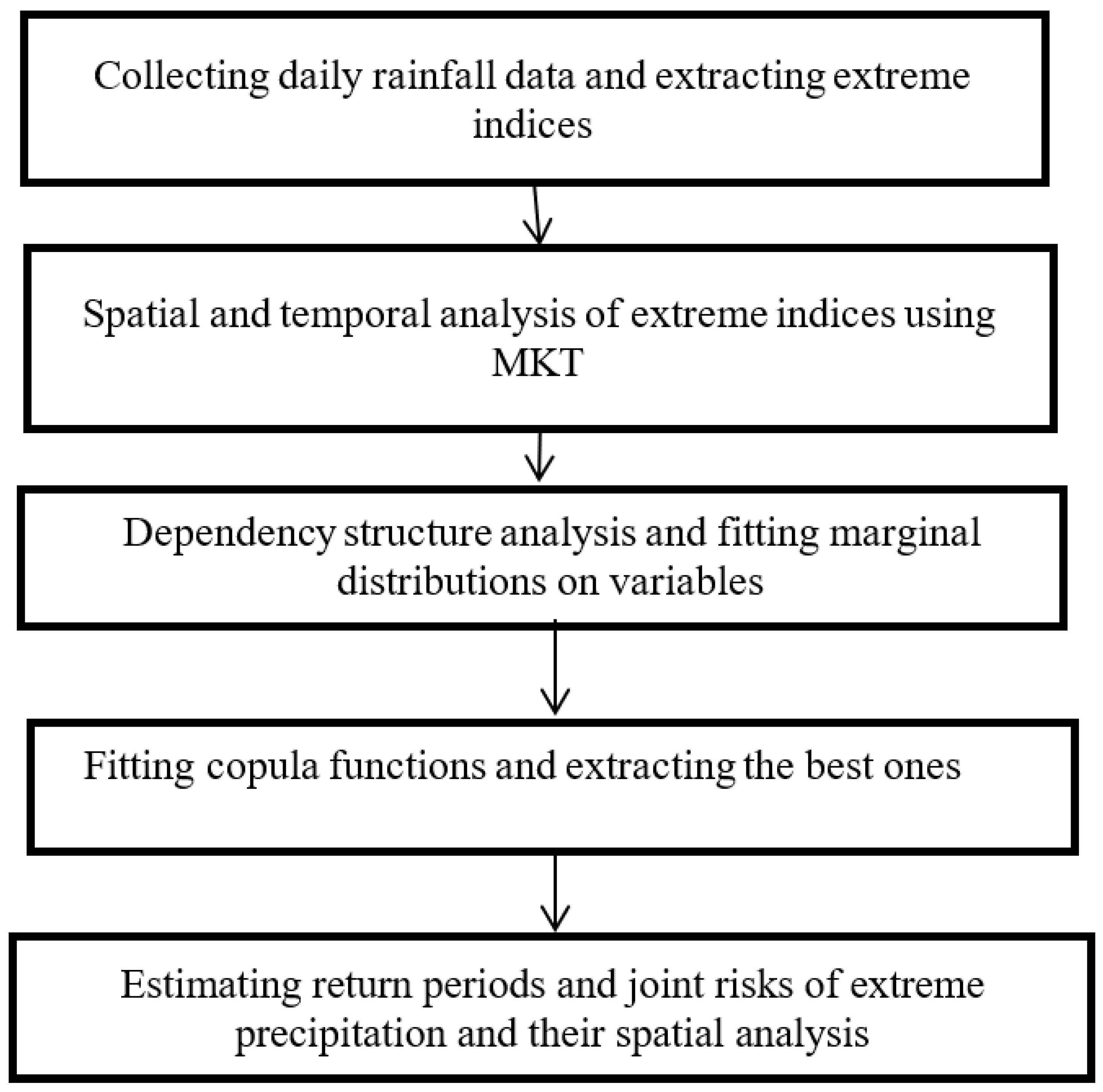
The study of extreme precipitation events is needed for risk management, policy making and planning in the agricultural sector, water resources management, and environmental resource management. To that end, it is necessary to analyze the probability of extreme precipitation characteristics, their joint probabilities, return periods, and their risk for various durations. The objective of this study, therefore, was to perform (1) a spatial and temporal analysis of extreme precipitation trends in Iran over the last five decades; (2) an analysis of univariate and multivariate probability behavior of extreme precipitation based on copula functions; and (3) an analysis of return periods and risk of extreme precipitation in Iran.
3. Results
3.1. Spatial Distribution of Extreme Indices
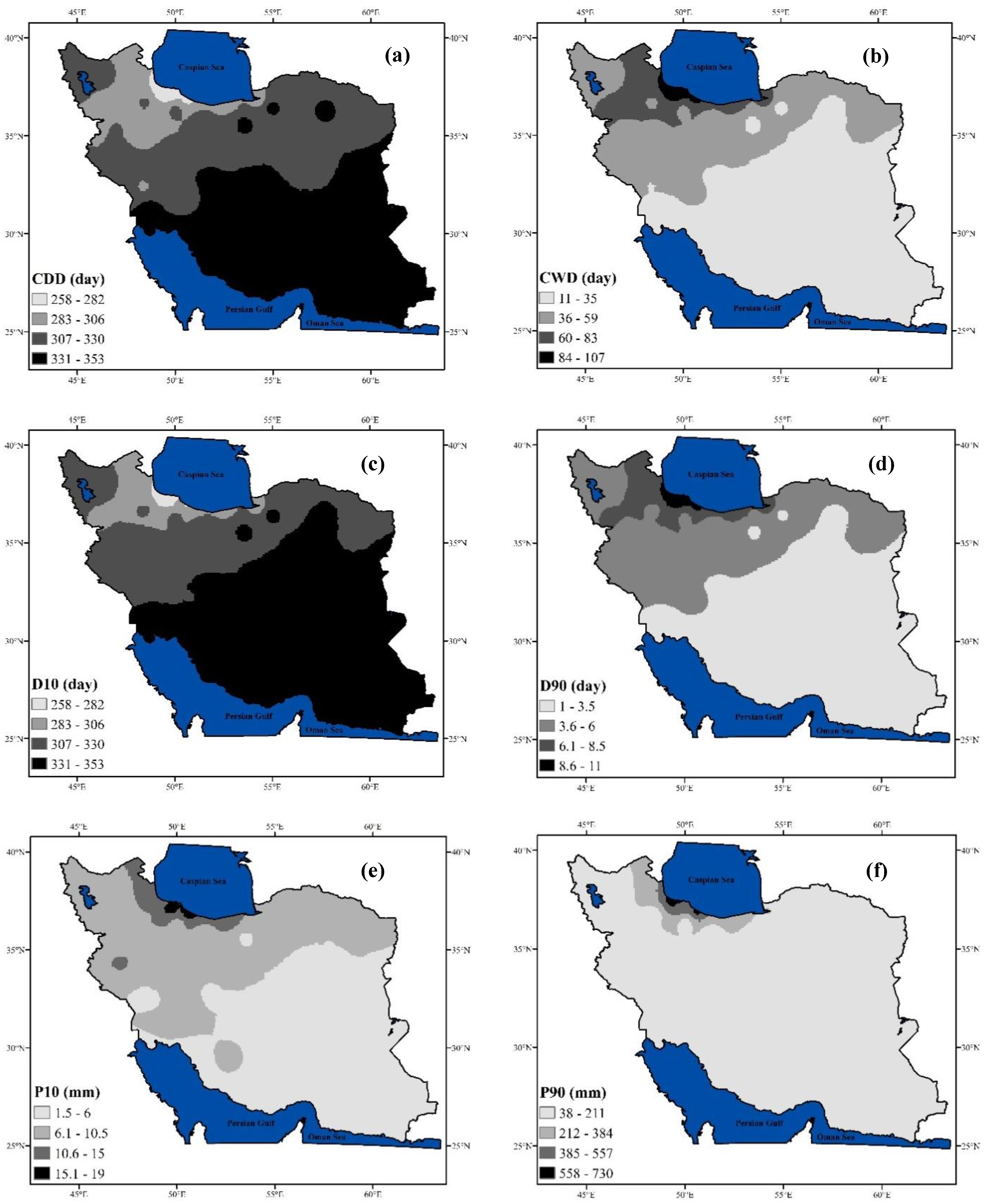
The spatial distribution of extreme precipitation, based on a long term average, is illustrated in
Figure 3. Generally, most parts of Iran, even the wet and severely wet climate regions in the north, experienced more than 9 months of dry days.
Most of the dry days belonged to the internal and coastal deserts (arid regions), which on average were from 331 to 353 days in a year (11.4 months of year). The semi-arid and Mediterranean regions of Iran (north eastern and north western) experienced 283 to 330 dry days, while northern Iran (wet regions) experienced around 9 months of dry days. In the analysis of CWD distribution, the highest frequency for most events belonged to northern Iran (3 months), whereas the southern and middle regions of Iran experienced less than one wet month. The spatial distributions of trends of D10 and D90 were similar to those of CWD and CDD. While D10 and CDD followed a similar distribution, heavy rainfall (greater than the 90th percentile, D90), on average, occurred for 3 days in the south and 10 days in the north of the country.
The minimum P10 index was 1.5 mm in Iran (in dry and desert regions) and the maximum P10 was about 19 mm in the Caspian coastal (north) area. The P90 index or flood precipitation was less than 211 mm in 90% of regions and was from 212 mm to 730 mm in the north and northwest regions of Iran.
3.2. Spatial Distribution of Univariate Indices
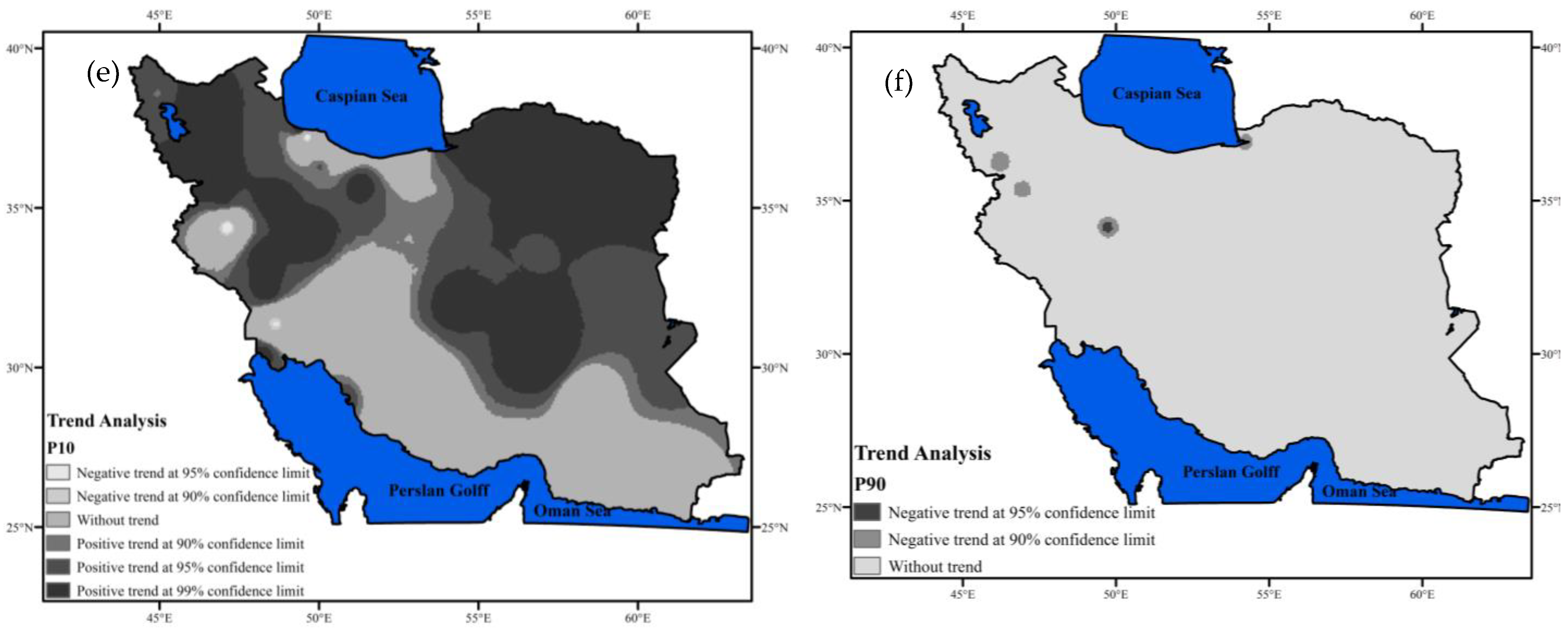
Figure 4 illustrates the trends of extreme indices that were calculated using MKT for the last 5 decades. As shown in
Figure 4a, there was no significant trend in the CWD (consecutive wet day) index in large parts of Iran, which includes arid and semi-arid regions. This index was negative for west, northwest, southwest, and a small part in the north of Iran. These regions include Mediterranean climate (west of Iran) and semi-arid and cold climate (northwest and southwest of Iran), which are generally affected by the Mediterranean Sea.
Figure 4b shows the CDD (consecutive dry days) trend. The trend of dry days increased in more than 92% of Iran. This increase was more intense in the west and the middle parts of Iran. The spatial distribution of D10 is represented in
Figure 4c, which shows that this index was increasing in large areas, including the west, north, and east of Iran. The trend was more severe in the north and west, while D90 was decreasing for the entire country.
Furthermore, P10 (
Figure 4d) followed an intensely increasing trend in the northwest and northeast regions, while the trend of P90 index (
Figure 4e) was not statistically significant. In a nutshell, the extreme precipitation indices indicated that the wet period was decreasing, while the dry period was increasing in Iran.
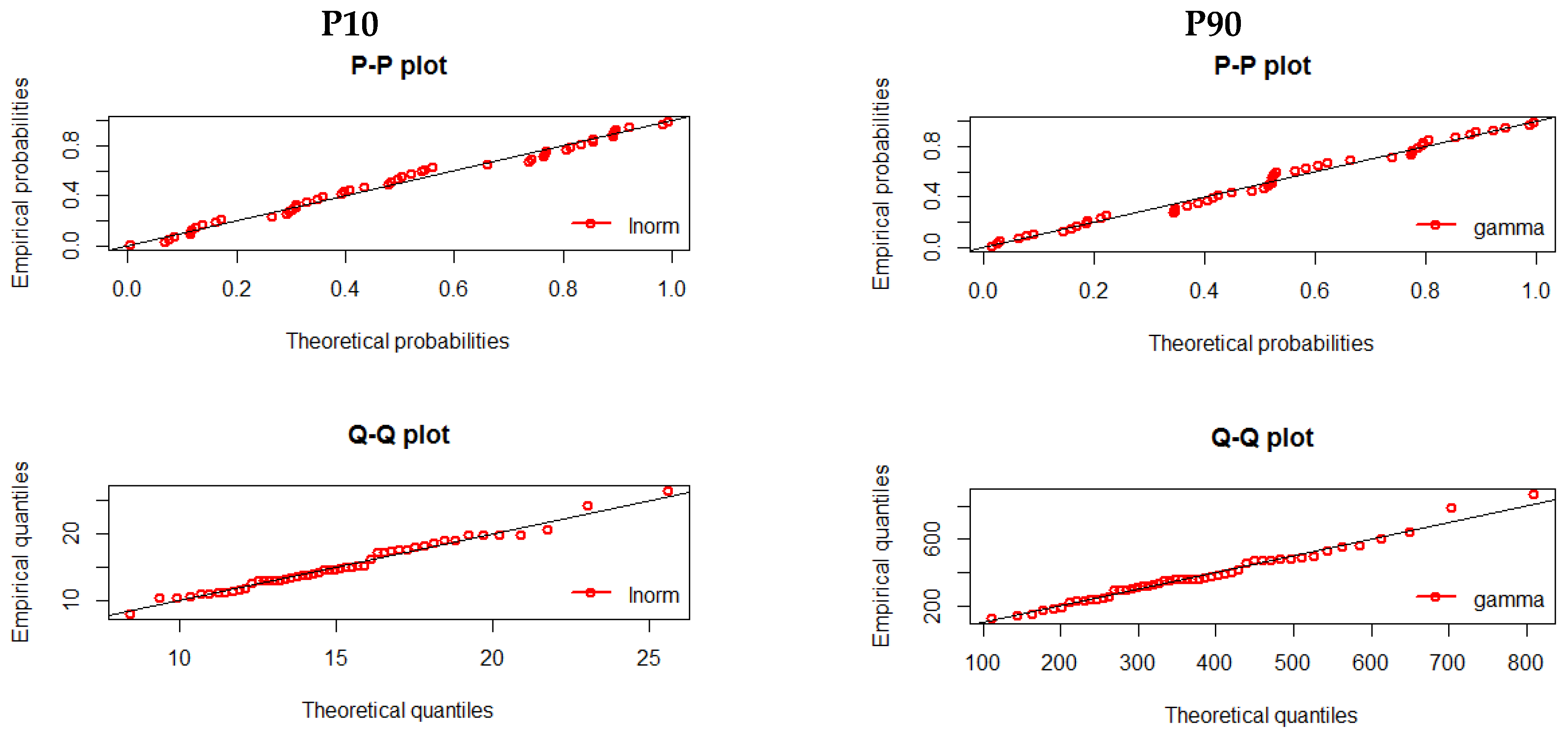
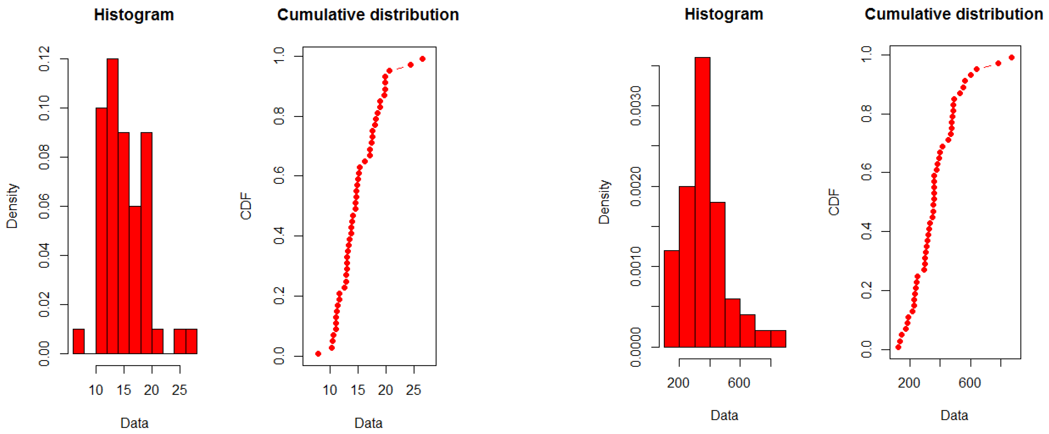
3.3. Marginal Distributions of Extreme Precipitation Indices
Discrete and continuous distributions were fitted to the extreme precipitation indices. The maximum likelihood estimation and L-moments methods were used, based on Student t, to estimate the parameters, and the accuracy of models was assessed using the AIC criterion and Chi-square goodness of fit test for continuous and discrete distributions.
Table 6 represents the parameters of discrete distributions fitted to CWD, CDD D90, and D10 indices, and
Table 7 displays the estimated parameters of P90 and P10 distributions for the Babolsar station (as an example).
The results showed that, on the basis of the AIC criterion, the negative binomial type I, Poisson, Poisson inverse Gaussian, and Poisson distributions performed best in modeling CWD, CDD, D10, and D90, respectively, while the log-normal and gamma distributions better fitted the P10 and P90 indices.
Figure 5 displays the quality of the fitted distributions for the P90 and P10 indices at the Bobolsar station based on graphical criteria.
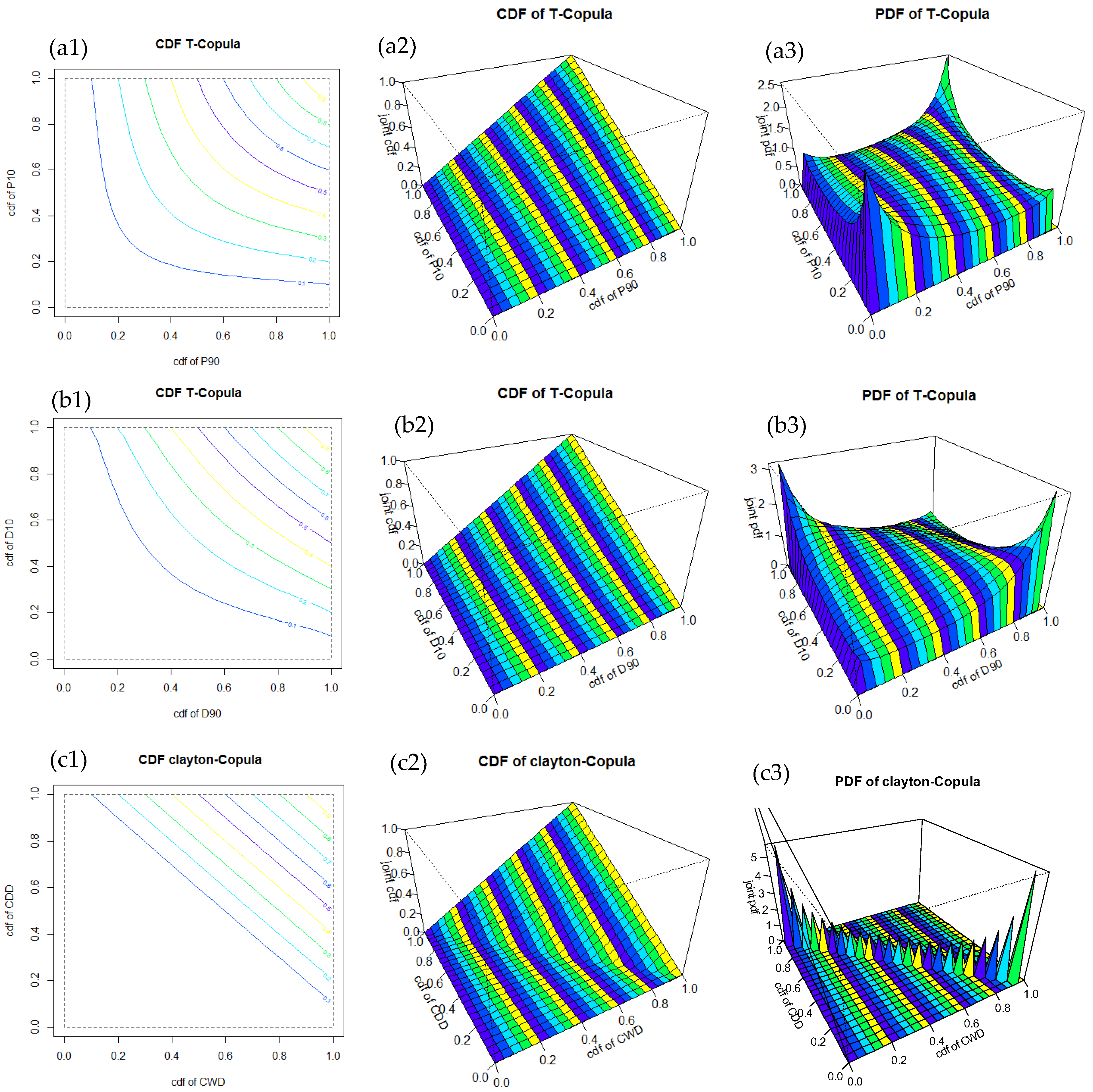
3.4. Dependency Structure between Extreme Indices and Fitting Copula Functions
The joint dependency between indices was assessed using Spearman, Kendall, and Pearson correlation coefficients.
Figure 5 displays the PDF, CDF, and alignment lines between the theoretical and empirical copulas at the Bobolsar station. The results showed that the t-copula performed better at the majority of stations. The spatial distribution of these indices is illustrated in
Figure 6a–d on the basis of Kendall’s tau. This figure shows a significant correlation between variables. After selecting the best marginal distributions and correlations, five copula functions belonging to the Archimedean and Elliptical families were used to construct the joint distribution of variables. The best copulas were determined, based on the Sn criterion, and the parameters of the copula function were estimated using the tau method.
Table 8 shows the fitted copulas and goodness-of-fit test for the studied variables at the Babolsar station.
Figure 7a–c shows goodness of fit graph for P10, P90; D10, D90 and CDD, CWD. We used from, contour plot, PDF and CDF of bivariate analysis. Based on Results, t-copula is best copula for all variables.
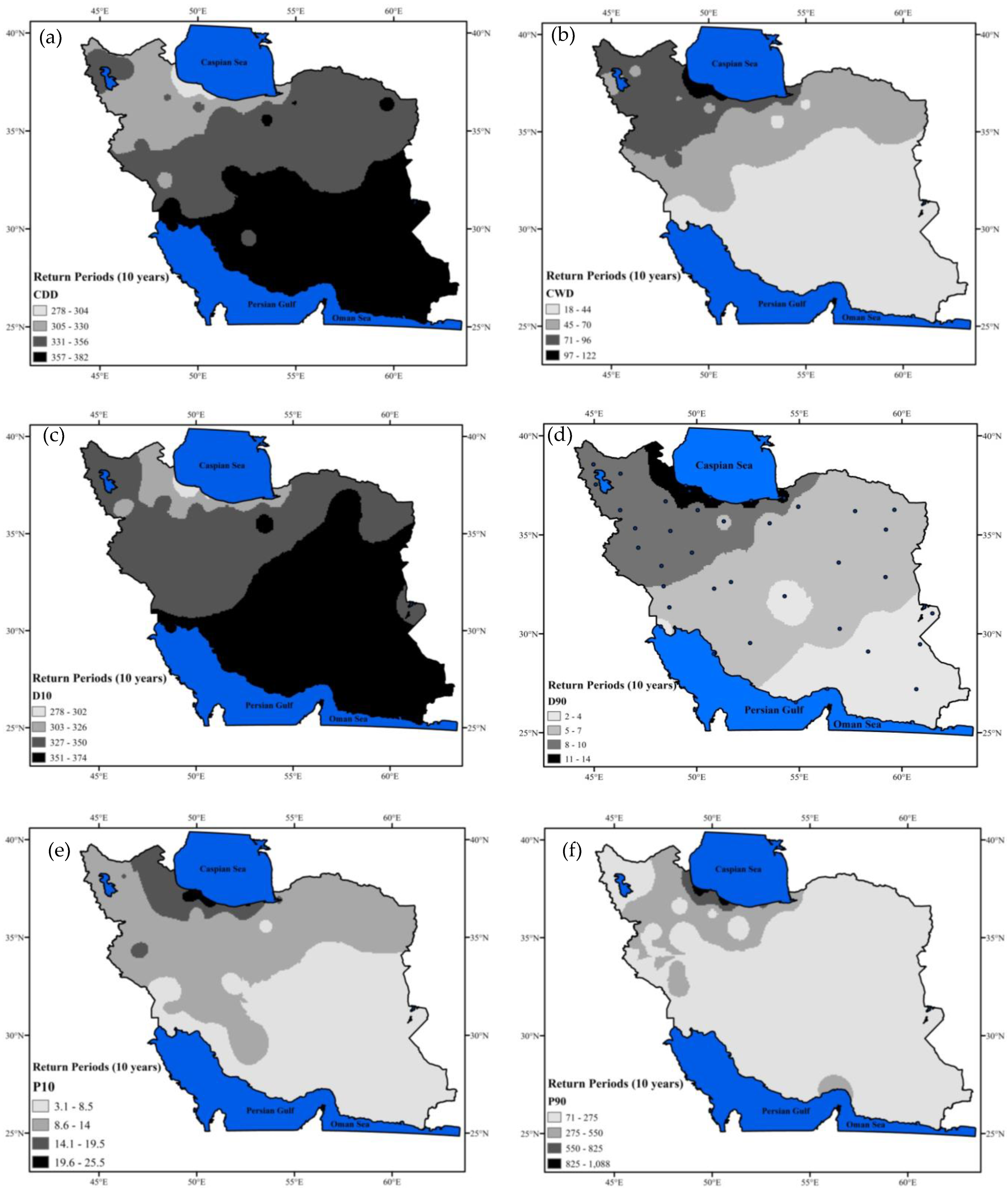
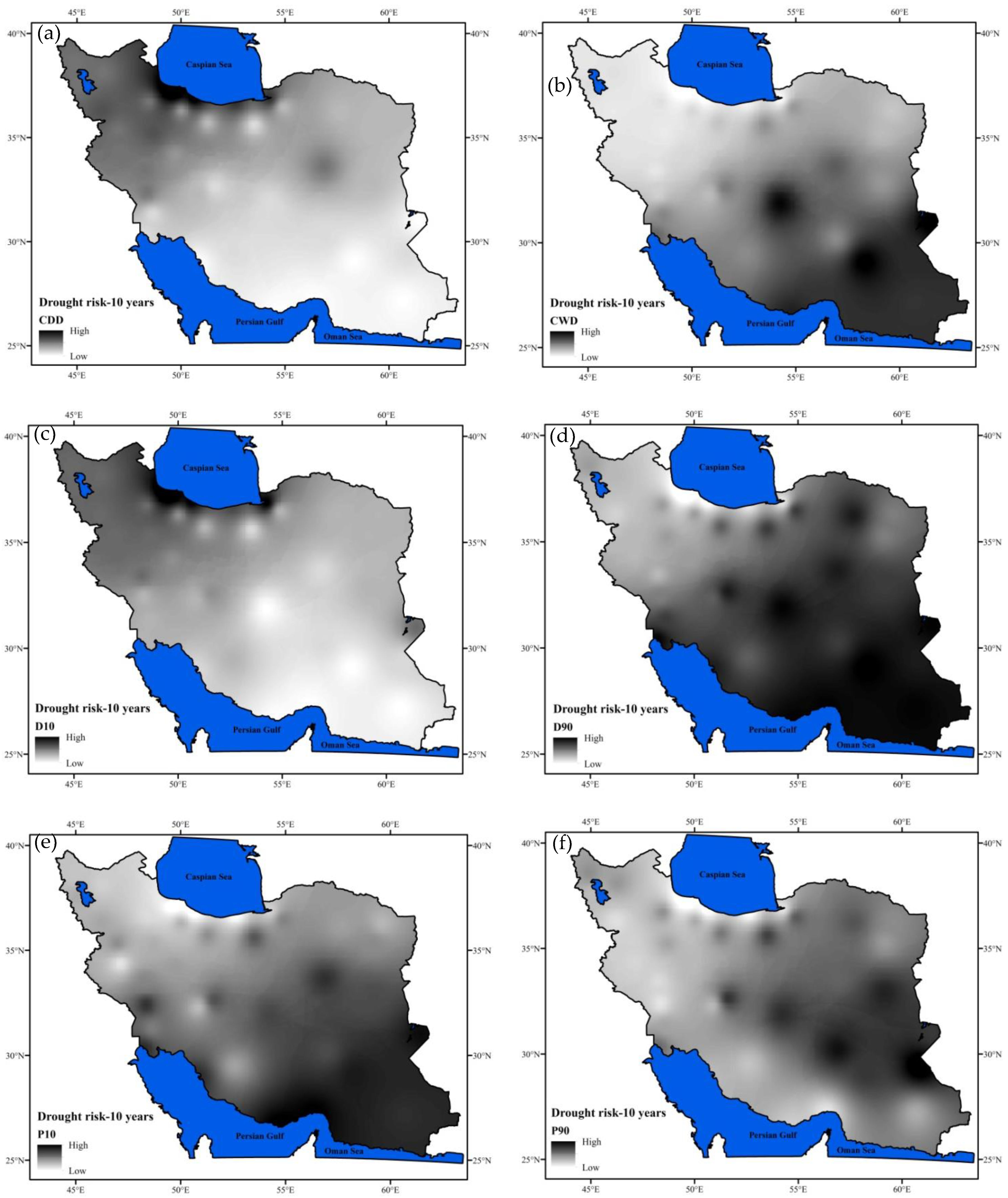
3.5. Spatial Analysis of Return Period and Risk of Univariate Extreme Indices
On the basis of the marginal distributions introduced in
Table 5, ten-year return periods and spatial risk analysis were estimated for all parts of the country, as represented in
Figure 8 and
Figure 9. For the CDD variable, the number of dry days with a 10 year return period increased from the northwest to the southeast of Iran (
Figure 8a), whereas the number of wet days increased from the southeast to the northwest of the country (
Figure 8a,b). This means that, on average, the southeast part of Iran faced 342 to 365 dry days and 18 to 44 wet days every ten years, while this was 278 to 299 dry days and 92 to 122 wet days for the northwest regions. Analysis of the two abovementioned indices (
Figure 9a,b) revealed that the south and southwest regions of Iran (central plateau and Hamoon basins) had a higher risk for the number of dry days, and the north and west regions (Mazandaran, Urumia and Karkheh basins) had the highest risk for the number of wet days.
Figure 8c indicates that most parts of Iran were faced with a significant increase in D90 (
Figure 8c). In other words, D10 increased sharply from northwest to southeast, while D90 increased slightly from south to north (
Figure 8d). Therefore, low rainfall in the middle and southern parts of Iran (high risk
Figure 9c) and heavy rainfall (
Figure 9d) in a limited part in the north of country were expected. In this regard, a large part of Iran was expected to face a continuation of the drought period, and a small part would see a continuation of the wet period. Furthermore, the highest risk of D10 was expected to occur in Mazandaran, Urumia, and the Karkhe basin, with the highest risk of D90 in the central plateau of Iran, Hamoon, Persian Gulf, and Oman Sea.
Figure 8e,f indicate that P10 and P90 had little variation. They reached their maximum in a small area in the north. Generally, in most regions of Iran the probability of low rainfall events increased (increased drought) and decreasing heavy rainfall was experienced. The P10 risk analysis map displayed in
Figure 9e shows that a large part of Iran had a high drought risk and only a small region in the north experienced low drought risk. In this regard, the P90 risk analysis map shown in
Figure 9f indicates that most regions of the country experienced a low and medium risk of flooding from heavy rainfall.
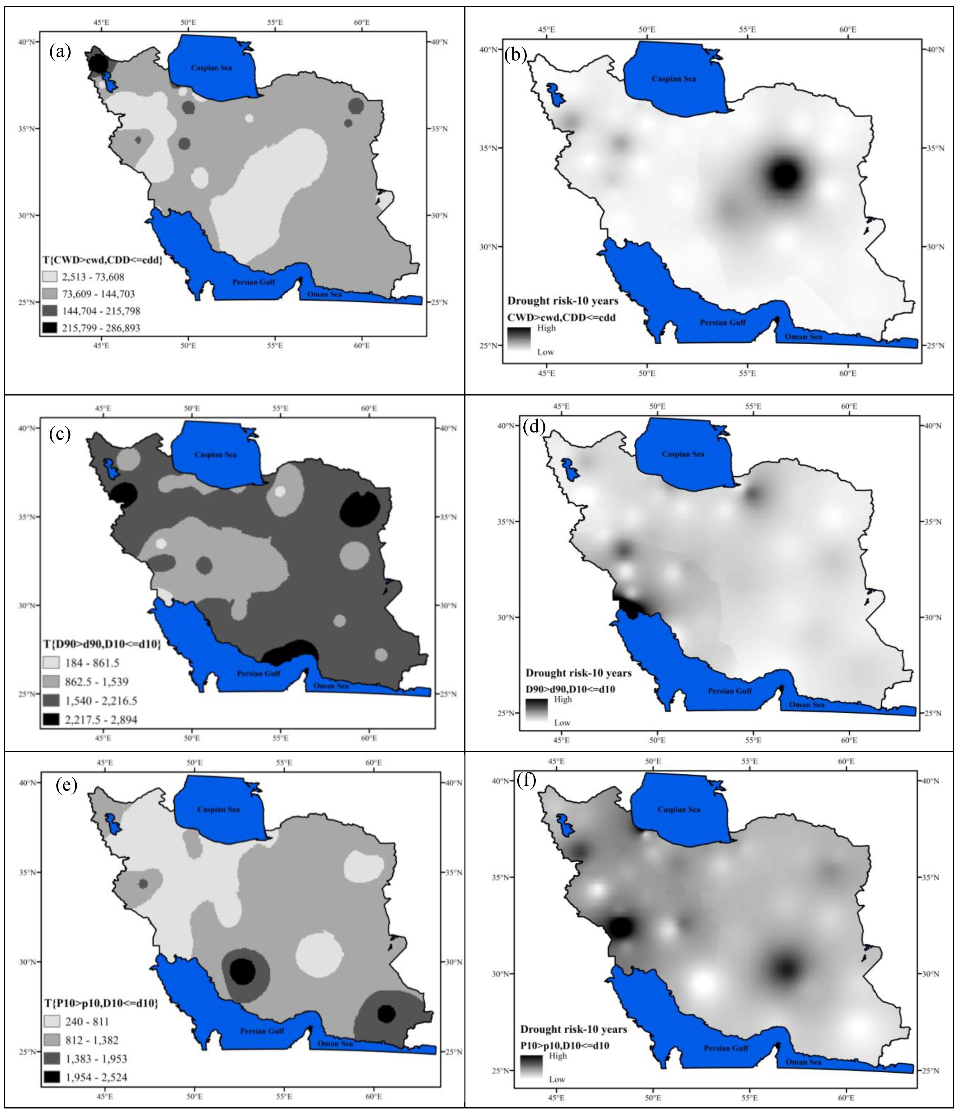
3.6. Spatial Analysis of Copula Based Extreme Indices
The spatial pattern of the bivariate return period and risk analysis obtained for the extreme precipitation indices is displayed in
Figure 10.
Figure 10a represents the spatial distribution of the bivariate return period that was obtained from
, with a higher return period corresponding to a lower probability of occurrence. Thus, as
Figure 10a shows, the simultaneous probability of CWD and CDD, and then the risk of occurrence, was very high (
Figure 10b). In addition, in parts of the northwest and the central desert and coastal desert in southwest of Iran, the return period was low (with high probability and high risk). Therefore, there was a possibility of extreme precipitation occurrences, such as heavy rainfall or long drought durations. Furthermore, in more than 50 percent of the region, the return period was less than 27.5 years, and hence the simultaneous probability of these two events was less than for 27.5.
Figure 10c displays the spatial distribution of the joint return period for
. As
Figure 10d shows, the joint probability of two events was high in the southeast, coastal, middle, and west parts of the Caspian Sea, with a return period of less than 116 years. In addition, the risk analysis of these variables indicated that a large part of Iran had a low or medium risk. In this regard, the Mazandaran basin in the north, Karkheh basin in the west, and Hamoon basin in the southeast of the country had a very high risk, in terms of heavy rainfall frequency and long drought duration.
Figure 10e,f show the possibility of the simultaneous assessment of heavy and weak rainfall events based on the joint risk and return period obtained from
.
These events were likely to occur within 24 to 64 years in the middle part of the Caspian Sea, and in coastal parts of the Persian Gulf and Oman Sea, while there was a high risk in the eastern part of Mazandaran and Karkheh basins.
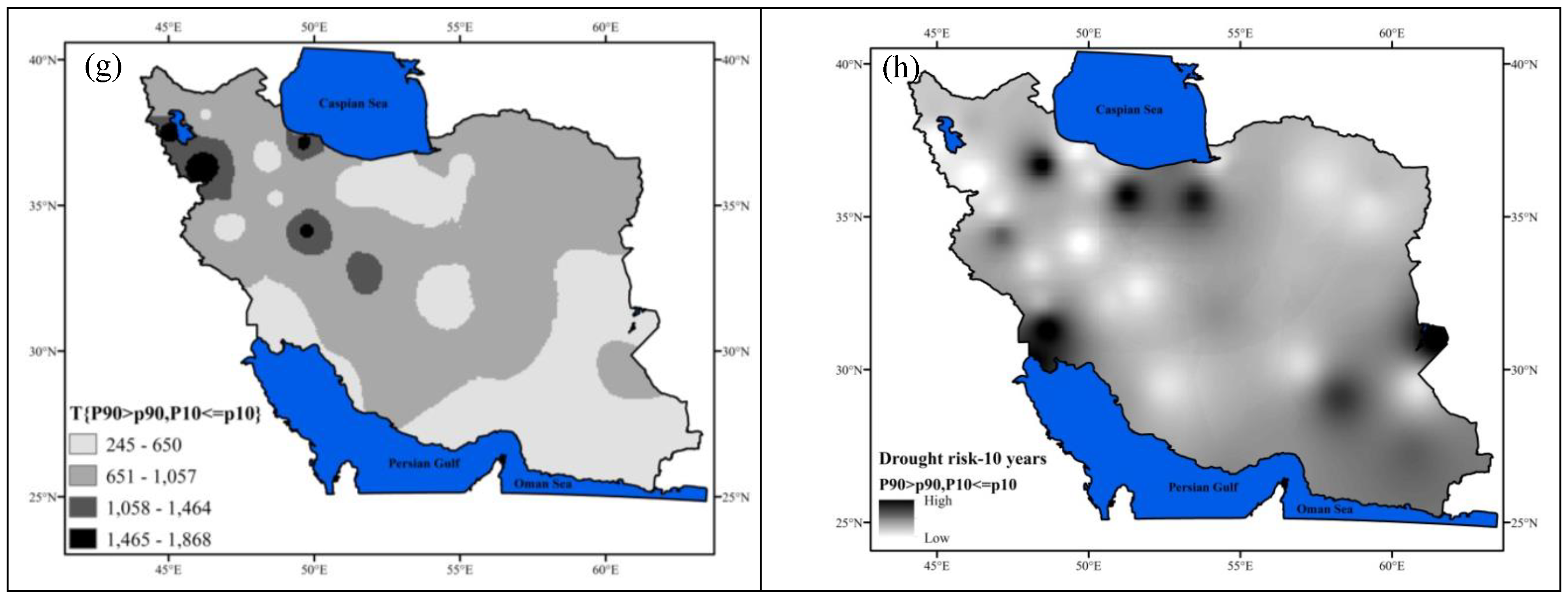
The spatial distribution of
represented in
Figure 10g indicates that there was a high possibility of a long drought duration with low rainfall occurrence. This figure also shows that the joint probability of P10 and D10 was high in the west and southwest regions, medium in the middle and east regions, and low in the southeast coastal region in Chabahar and some parts of Fars province. In this regard,
Figure 10h represents a high risk in some parts of Kerman in the Lut desert (central basin) and some parts of Karkheh basin and its inlet in the western province of Iran.
4. Discussion
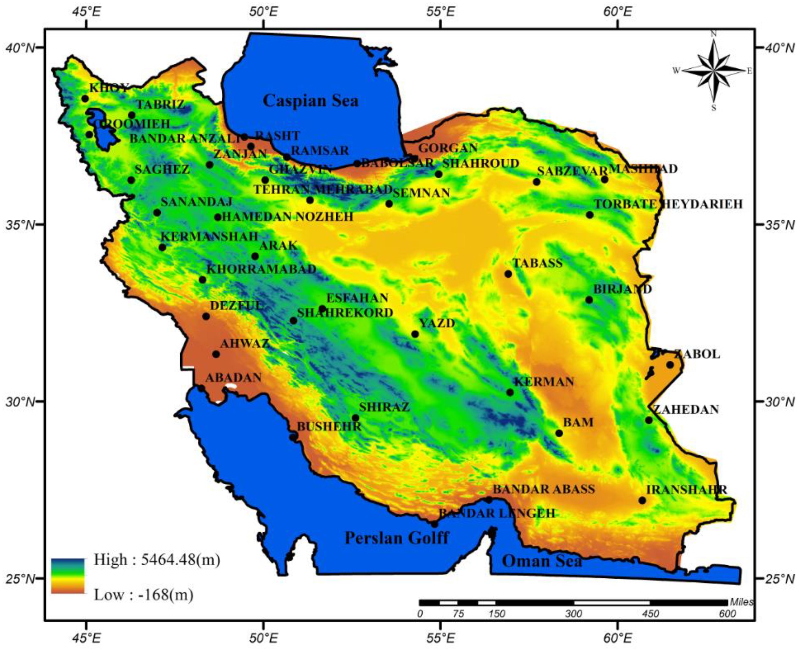
The current research aimed to perform univariate and bivariate analyses of extreme precipitation indices in Iran. Iran is a vast country with a diverse climate, where frequent floods/droughts affect various sectors, such as agriculture, the environment, roads, urbanization and construction, reservoirs, and natural resources.
The results of the analyses showed that the probability of CDD occurrence in Iran tended to increase and CWD tended to decrease. For more than 70% of the area, in western, eastern, and southern parts, the annual number of days with precipitation less than 1 mm was more than 322 days per year.
Alexander et al. [
39] showed that the CDD was relatively decreasing at most stations in the continental part of the Earth during 1951–2003, which can be interpreted as similar to the prediction of the Intergovernmental Panel on Climate Change (IPCC). In most parts of Iran, the possibility of occurrence of CDD is increasing, which has been reported by Alijani et al. [
40], Razie et al. [
41], and Asgari et al. [
42]. In this sense, Iran will be subjected to increasing risks of drought hazard.
The trend of CDD is increasing in more than 92% of Iran, as confirmed by Soltani et al. [
43] Asgari et al. [
42]; Tabari et al. [
9]; and Balling et al. [
10]. In this regard, there was no significant trend in the south and southwest of the country. Precipitation in these regions was under the effect of separate synoptic systems, including the monsoon low-pressure system, Persian Gulf, Oman Sea, and Red Sea [
44].
In west and north of Iran, CWD is increasing, showing a higher risk of heavy rains and a higher risk of floods There was no significant trend in the CWD (consecutive wet day) index in large parts of Iran, including arid and semi-arid regions. According to Heydari and Khoshakhlagh [
45], the increasing atmospheric pressure and temperature in Mediterranean Sea over last 60 years are the causes of a comprehensive drought in the western half of Iran. Based on climate change models, this situation will continue for the next half century.
Alexander et al. [
39] showed that few stations on Earth recorded increasing CWD. In Iran, a small number of stations, such as at Bandanzali, Rasht and Khoi, showed the possibility of an increasing CWD. The results of Asghari et al. [
42] and Alavinia and Zarei [
25] also showed similar results.
The spatial distribution of joint probability of P90 and D10 represents that there was a high possibility for longer drought durations with low rainfall occurrence in the west and southwest of Iran and heavy rainfall in the Mazandaran basin in the north, Karkheh basin in the west, and Hamoon basin in the southeast of Iran. Reports from the IranWRM [
45,
46] confirmed the above analysis, such that severe flooding caused huge damage in Karkheh basin during the years 2013, 2015, 2018, and 2019; in Mazandaran basin during 2015, 2017, 2018, and 2019; and in Hamoon basin during 2017, 2019, and 2020.
5. Conclusions
This study performed a spatial and temporal analysis of extreme drought indices in Iran using the MKT test and copula functions. The results of the study are as follows:
Low rainfall duration and consecutive dry days (CDD) were increasing from northwest to the southeast of Iran, while consecutive wet days (CWD) were decreasing, such that the severity of this trend was very high in the southeast and northern parts of the country (Mazandaran, Urumie, and Karkheh sub basins). The P10 and D10 indices were decreasing in the southern and northern coastal regions and increasing in the northwest and southeast of Iran. However, heavy rainfall (P90 and D90) did not follow a regular pattern. In summary, it can be concluded that the wet and Mediterranean regions in the north, west, and northwest of the country were tending to severely dry out, whereas the arid and semiarid regions of Iran tended to dry out moderately.
More than 50 percent of Iran experienced low risks with a return period of extreme indices (CWD, CDD) of more than 27.5 years. In this regard, the joint return periods of (D10, D90), (P10, P90), and (D10, P10) pairs were less than 100 years in most regions of the country.
Furthermore, the return period in the western, northern, and northwest parts was very low, so the risk was very high. These regions included the Mazandaran basin in the north and Karkheh basin in the west and northwest of Iran.
The joint probability of dry and wet events is an efficient tool for warning of drought/flood conditions, because extreme precipitation events have negative impacts on water resources, soil moisture, and water quality. Finally, due to the variability of extreme precipitation events in recent years, the findings of this study are useful for reducing the impacts of drought/flooding and the changing environment.


 ,
, 


