
Atmospheric Response to EEP during Geomagnetic Disturbances
by
 , , and
Dmitry Grankin
1,
Irina Mironova
1,*,
Galina Bazilevskaya
2,3,
Eugene Rozanov
1,4 and
Tatiana Egorova
4 1
Faculty of Physics, St. Petersburg State University, 199034 St. Petersburg, Russia
2
Lebedev Physical Institute, Russian Academy of Sciences, 119991 Moscow, Russia
3
Skobeltsyn Institute of Nuclear Physics, Moscow State University (SINP MSU), 11991 Moscow, Russia
4
The Physikalisch-Meteorologisches Observatorium Davos, World Radiation Center, 7260 Davos, Switzerland
*
Author to whom correspondence should be addressed.
Atmosphere 2023, 14(2), 273; https://doi.org/10.3390/atmos14020273
Submission received: 30 December 2022
/
Revised: 21 January 2023
/
Accepted: 27 January 2023
/
Published: 30 January 2023
(This article belongs to the Section Upper Atmosphere)
Abstract
:Energetic electron precipitation (EEP) is associated with solar activity and space weather and plays an important role in the Earth’s polar atmosphere. Energetic electrons from the radiation belt precipitate into the atmosphere during geomagnetic disturbances and cause additional ionization rates in the polar middle atmosphere. These induced atmospheric ionization rates lead to the formation of radicals in ion-molecular reactions at the heights of the mesosphere and upper stratosphere with the formation of reactive compounds of odd nitrogen NOy and odd hydrogen HOx groups. These compounds are involved in catalytic reactions that destroy the ozone. In this paper, we present the calculation of atmospheric ionization rates during geomagnetic disturbances using reconstructed spectra of electron precipitation from balloon observations; estimation of ozone destruction during precipitation events using one-dimensional photochemical radiation-convective models, taking into account both parameterization and ion chemistry; as well as provide an estimation of electron density during these periods.
1. Introduction
The state of the ozone layer has recently attracted the attention of society in connection with the noted trends in the decrease in its global content since the end of the 20th century [1,2] and the understanding of its role not only as a protector of life on Earth from the harmful effects of the hard part of the ultraviolet radiation of the Sun, but also as a factor influencing climate and the biosphere as a whole [3]. The ozone measurement shows that, despite the measures taken to limit the anthropogenic impact on the ozone content, its recovery is slower than expected, and its significant reduction continues in some regions [4]. Of particular concern is the emergence of a vast ozone hole over the Arctic in 2020 [5], mini-ozone holes [6,7]. These facts make a detailed study of the dependence of the state of the ozone layer on natural factors, such as solar and geomagnetic activity, timely and relevant. Processes in the upper layers of the atmosphere, in particular, can significantly affect the variability of stratospheric ozone in the polar mesosphere and lower thermosphere. The results of recent studies have shown [1,8] that energetic electrons of magnetospheric origin have a significant impact on the behavior of the ozone layer and climate.
Energetic electron precipitation (EEP) from the outer radiation belt is associated with solar activity and space weather and plays an important role in the Earth’s polar atmosphere and can be observed by satellites and balloon measurements. The precipitating electrons are absorbed in the upper atmosphere, but they generate the X-ray bremsstrahlung that can be detected by balloons down to the height of 20 km and even lower. Although information on precipitation is currently obtained from measurements on satellites, the results of balloon observations have not lost their significance, since electrons from the radiation belt can escape both into the atmosphere, and into interplanetary medium [9,10]. Balloons detect radiation in the atmosphere in situ. This is important not only for studying the response of the atmosphere to electron precipitation, but also for assessing the radiation hazard on aircraft routes [11,12]. Nowadays, the balloon measurements of X-rays from precipitating electrons are carried out in conjunction with measurements on satellites [13,14].
Information about electron density usually considers from the F2 layer (about 400 km) up to the D layer (about 60 km) of the ionosphere and is measured, for instance, by radars and VLF transmitters [15,16]. The X-ray bremsstrahlung from EEP observed by balloons gives the possibility to estimate the variability of the electron concentration at altitudes below 60 km.
Energetic electrons from the radiation belt precipitate into the atmosphere during geomagnetic disturbances and cause additional ionization rates in the polar middle atmosphere [1,2,17,18,19,20,21,22]. These induced atmospheric ionization rates lead to the formation of radicals in ion-molecular reactions at the heights of the mesosphere and upper stratosphere with the formation of reactive compounds of nitrogen NOy (N, NO, HNO3, HNO4, ClNO3, N3O5, NO2, NO3) and hydrogen HOx (H, OH, HO2). These compounds are involved in catalytic reactions that destroy the ozone [1,2,23]. In the polar atmosphere, ozone losses can reach about 30% in the upper stratosphere and up to 80% in the mesosphere during periods of strong geomagnetic storms [1,2,23].
The power of geomagnetic disturbances or storms is often determined using different geomagnetic indices, such as AE, Kp, and Dst, which are measured at different latitudes. For our study, we took into account geomagnetic disturbances according to the Kp index.
The information about the precipitation of energetic electrons (energy spectra and particle fluxes) makes it possible to calculate atmospheric ionization rates. EEP from the outer radiation belt in the subauroral region causes an increase in the ionization rate in the atmosphere from the upper boundary to a height of about 20 km via the EEP bremsstrahlung [24]. Using the atmospheric ionization rates during geomagnetic disturbances with the help of radiation-convective-photochemical models, it is possible to estimate the destruction of the ozone and electron concentration in the field atmosphere associated with EEP.
The role of energetic electrons precipitating from the radiation belts in ozone variations and climate changes is still not clear due to the fact that the real ionization rates of the upper and middle (below about 120 km) high-latitude atmosphere under the influence of these particles are not known in detail [25]. One of the controversial issues raised is also related to the range of electron energies that may be most or least important for variations in atmospheric chemical changes, which in turn lead to local climate changes [8]. This necessitates studying the precipitation of energetic electrons (from 30 keV to several MeV) during geomagnetic disturbances.
The aim of this study is to explore the ozone layer, considering the influence of natural factors, such as precipitation of energetic particles from near-Earth space, taking into account the calculation of atmospheric ionization rates during precipitation of energetic electrons using reconstructed spectra from balloon observations. Estimation of ozone destruction and electron concentration during EEP uses one-dimensional photochemical radiation-convection models with ion parametrization and ion chemistry.
2. Materials and Methods
Since 1957 at the Lebedev Physical Institute (LPI), balloon measurements of ionizing radiation in the atmosphere have been regularly carried out [26,27,28]. Balloon facilities measure the fluxes of secondaries from galactic cosmic rays, solar protons entering the atmosphere during events of energetic solar particles, as well as bremsstrahlung of electrons when they drop from the outer radiation belt to the polar atmosphere of the Earth.
About 600 cases of electron precipitation were detected during the 1963–2020-observation period. The main regularities of the observed precipitations are described in [26,27,28]. It was shown that EEP mainly occurs on the descending branch of the 11-year solar cycle, against the background of high-speed solar wind streams from coronal holes, during moderate geomagnetic storms. There is a seasonal wave in the rate of EEP cases with peaks during the winter and summer equinoxes. In addition, a long-term trend in the rate of EEP was found, and it was suggested that this trend is associated with a constant increase in the number of active low-frequency radio transmitters [29]. To estimate the ionization rate in the atmosphere, it is necessary to have information about the magnitude of the flux and the energy spectrum of precipitating electrons. Balloon measurements provide information on the fluxes of X-ray bremsstrahlung at different layers of the atmosphere generated by precipitating electrons at higher layers. The transition from the measured X-ray fluxes to the energy spectrum of precipitating electrons at the boundary of the atmosphere is based on the simulation of the passage of primary and secondary electrons, as well as X-rays through the atmosphere by the Monte Carlo method [26]. The reconstructed spectra are in reasonable agreement with the spectra derived from the POES satellites measurements [30].
For this work, typical cases of precipitations of medium power were selected. The only selection criterion was the absence of fluctuations in the count rates of the detector. Strong temporal variations, including those on a minute basis, are inherent in precipitating electron flows [23]. However, fluctuations make it impossible to correctly find the spectrum of precipitating electrons from the LPI measurement, because the spectrum is determined from the absorption of the bremsstrahlung flux in the atmosphere under the assumption that the electron flux remains unchanged during the measurement time. Therefore, cases were chosen when a monotonic dependence of the X-ray flux on altitude was observed in the balloon flight. In the selected cases, the reliable observations of EEP were taken for at least 30 min. It should be noted the fact of EEP being recorded while the balloon is in this place, but there is no information about the actual beginning and end of the process, neither on the real space area covered by EEP.
Table 1 shows 4 cases of EEP events surrounded by geomagnetic disturbances with Kp = 4 according to balloon observations over Apatity (67.57 N, 33.56 E, McIlwain parameter L = 5.3). In Table 1, the time of balloon observation is indicated. For the modeling, the beginning and duration of EEP in this study are determined by the time of registration of increased geomagnetic disturbances Kp = 4.
2.1. Simulation of Ozone Depletion
This work uses two versions of the one-dimensional radiative-convective-photochemical model with parameterized and interactive ion chemistry. Both versions of the model cover the altitude range from 0 km to 120 km above the Earth’s surface in the area of observations and make it possible to estimate changes in the composition of the atmosphere after EEP.
2.1.1. Model with Standard Parameterization
The impact of EEP and the secondary electrons formed by them ionize neutral air molecules, leading to the formation of odd hydrogen HOx and odd nitrogen NOy [31,32,33]. Observation of these components in regions with increased ionization makes it possible to evaluate the intensity of the action of energetic electrons and the magnitude of the decrease in the ozone concentration.
The generation of the main positively charged ions can be represented by the following relationships:
With P(X) being the production of X and Q being the ionization rate.
According to the parametrization from [31,32,33,34], the combination of neutral and ionic chemistry processes leads to the formation of ~1.25 nitrogen atoms per ion pair, from which:
- ~0.7 molecules of excited nitrogen N(2D), which instantly reacts with neutral oxygen to form NO:
- ~0.55 NO2 molecules
The formation of HOx is given as a function of the height and ionization rate [33]. On average, one H atom and one OH molecule are formed per ion pair (but this ratio changes with height).
2.1.2. Ion Chemistry Model
The interactive ion chemistry version of the model includes 43 neutral gas impurities, electrons, and 57 positively and negatively charged ions [31,32,33,34]. In this case, the formation of calculations of changes in the chemical composition occurs interactively and the influence of energetic particles affects not only NOy and HOx, but also other neutral impurities belonging to the hydrogen, nitrogen, and halogen groups.
For example, nitric acid (HNO3) can be obtained from a simple reaction
or a complex chain of ionic/neutral chemical reactions ending with the destruction of the protonated water clusters:
3. Results
3.1. Obtaining Spectra and Ionization Rates
To reconstruct the atmospheric ionization rate, it is necessary to have information about the energy spectra (particle energy and flux intensity) and the parametrization of ion production. The calculation of the EEP ionization rates requires knowledge of the parametrization of ion production in terms of the atmospheric response function [19,20,21]. The computation ionization rates of the selected events are partially presented [17]. The function of the atmospheric response to EEP, at a certain depth of the atmosphere, is the number of ion pairs created by one precipitating electron with an initial energy at the upper boundary of the atmosphere. In this work, we used modified functions for monoenergetic electrons with initial energies from tens of keV to several MeV [19]. This model considers both direct ionization by primary electrons and secondary bremsstrahlung [19].
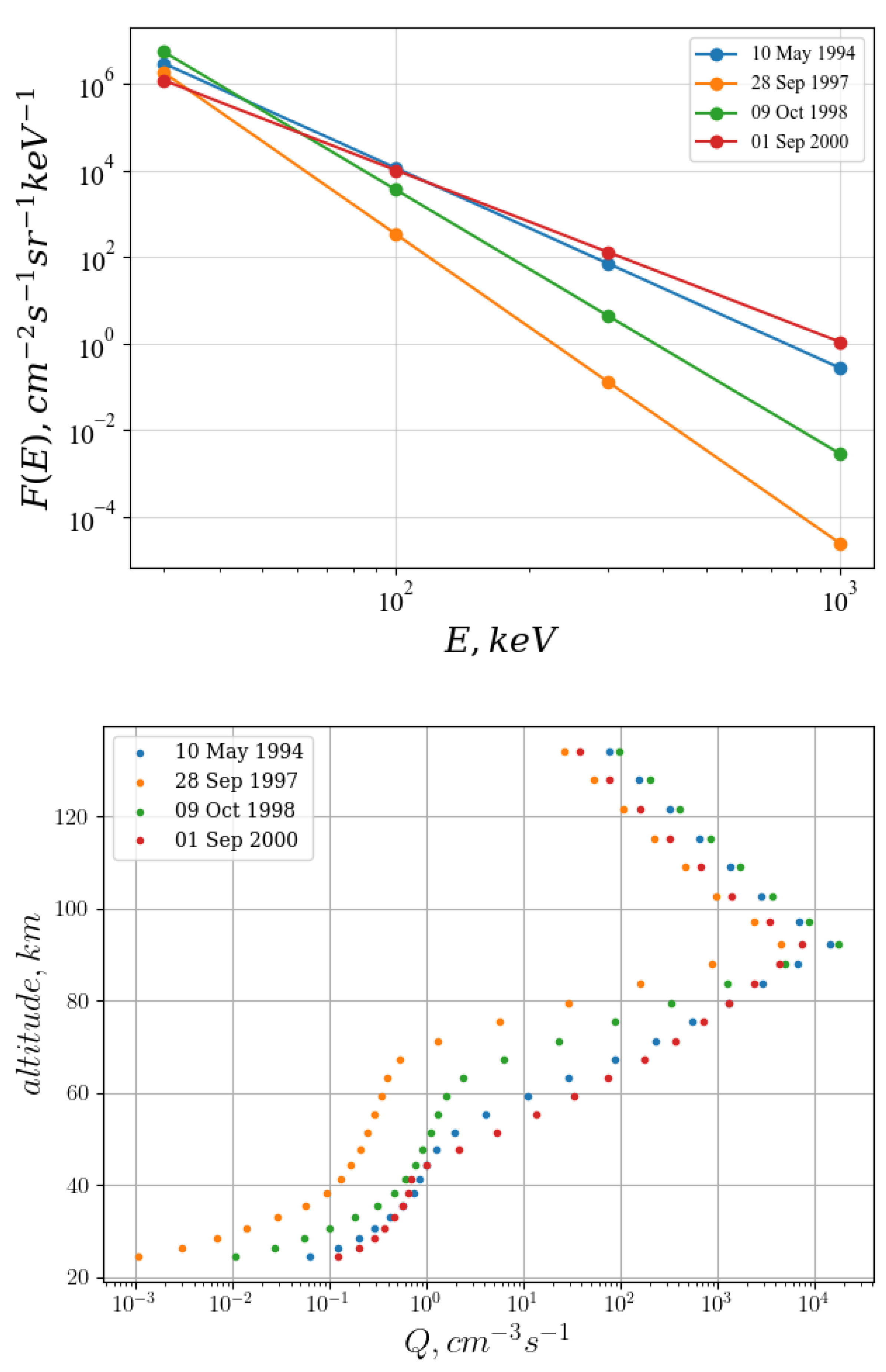
In Figure 1, upper panel, the EEP spectra with power low energy distribution F(E) = F(0)E−k for four selected cases, see Table 1, are shown. EEP was observed by balloon observations over Apatity (67.57 N, 33.56 E, L = 5.3) during geomagnetic disturbances with Kp = 4. It can be seen here that during geomagnetic disturbances, the intensity of the differential electron flux with energy of 30 keV exceeds 106 cm−2s−1sr−1keV−1. The intensity of the differential flux for 100 keV is about 104 cm−2s−1sr−1keV−1.
The ionization rate for the period under study was calculated considering the spectra presented in Figure 1. The calculation of the atmospheric ionization rate Q (number of ion pairs/gram/second) at a certain height (h), for all energies of electrons precipitating into the atmosphere, takes into account F(E)—the electron flow with kinetic energy (E) at the upper boundary of the atmosphere and the response functions of the atmosphere Y(E,h) on the precipitation of a monoenergetic single electron flux [19,20,21].
3.2. Model Results
To study the effect of EEP on the chemical composition of the atmosphere, four characteristic events were selected from the EEP recorded during balloon observations, see Table 1. The calculated ionization rates were introduced into the model, taking into account the duration of the geomagnetic disturbance, since the data of balloon measurements do not contain information on the duration of the event. So, for example, on 10 May 1994, the geomagnetic disturbance with Kp = 4 lasted for 9 h during the time period of 00 h–21 h (Table 1), so the ionization rates reconstructed from balloon observations affected the chemical composition of the atmosphere during 9 h.
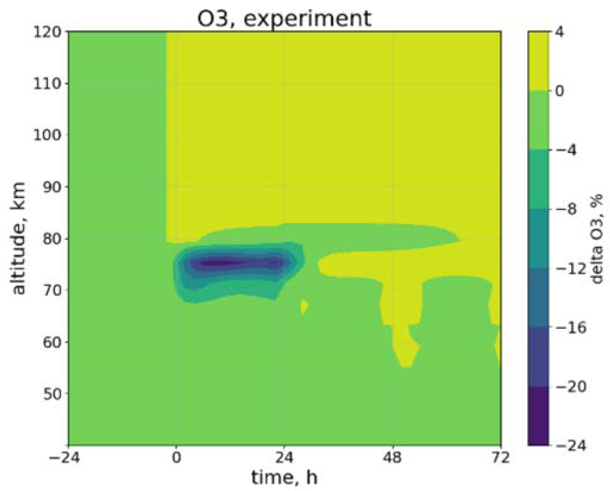
Figure 2 shows the EEP-induced ozone change calculated using a radiative-convective model with interactive neutral and ion chemistry.
Figure 2 demonstrates that the main ozone depletion, up to 24% compared to the quiet period, occurs at an altitude of 75 km. In addition, it can be seen that after ozone recovery (after ~30 h), a certain cyclic process occurs, which is associated with diurnal variations in the ozone content in the atmosphere (at these altitudes, ozone accumulates at night, and is destroyed during the day). Ozone decreases at altitudes below about 80 km, which is caused by losses due to enhanced HOx catalytic cycles [2,24]. These cycles require atomic oxygen to be excited; atomic oxygen below 80 km is only abundant during daytime when it is produced in the photodissociation of O2. The above graph allows us to select for further study the level of 75 km, where the most significant decrease in ozone occurs.
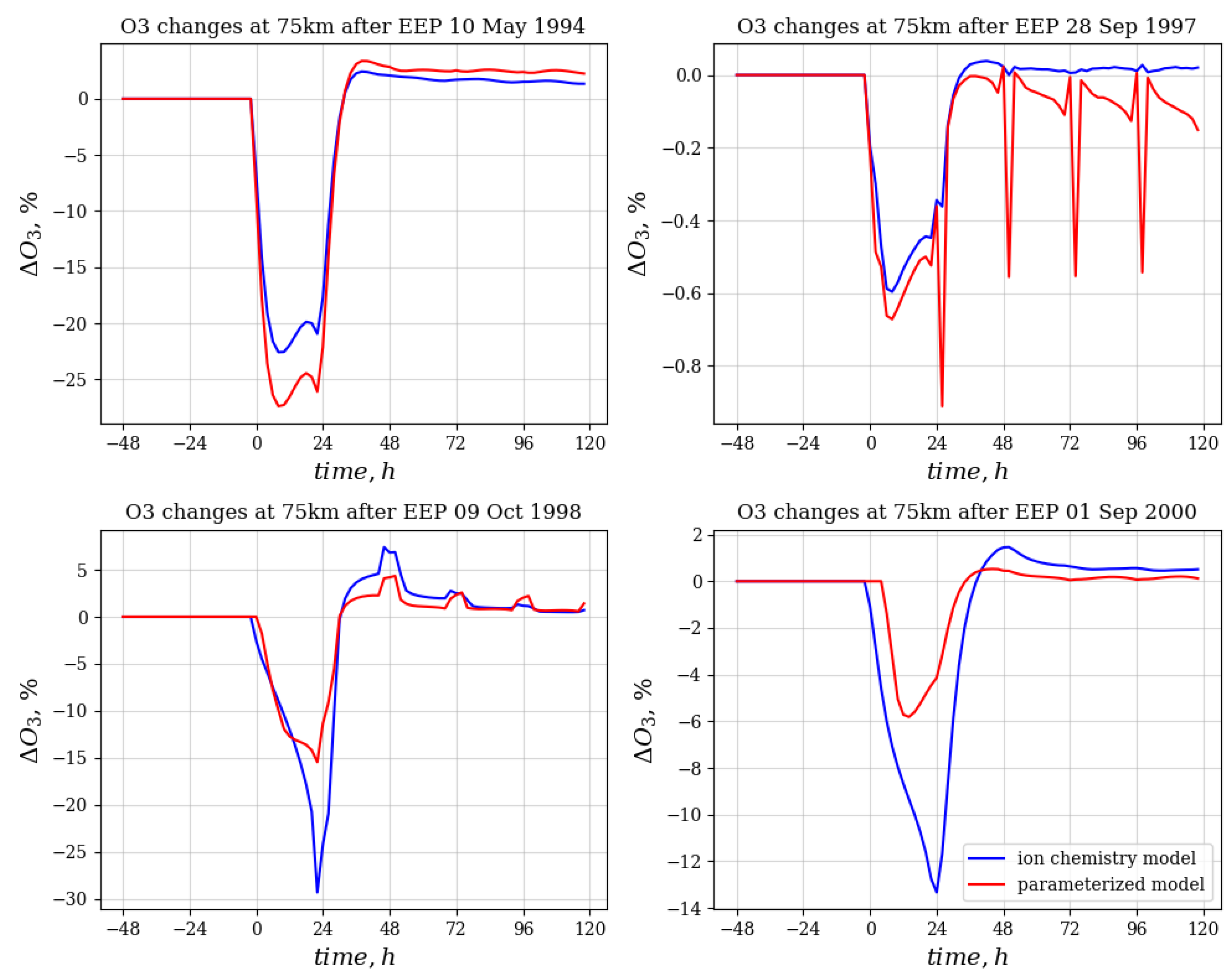
Let us consider the change in the content of ozone, HOx, NOy at an altitude of 75 km for all events listed in Table 1. The ionizing effect is specified in the model according to the periods when Kp = 4. In Figure 3, Figure 4 and Figure 5, the results of numerical simulation of the change in NOy, HOx are presented in the form:
and for the ozone calculated by the formula:
where Xexperiment and Xreference are the values of the volume fraction of the ozone mixture for the case with a disturbed (taking into account the ionization rate from EEP) and undisturbed atmosphere (without an EEP event). Mixing ratios are in ppbv (“parts per billionth volume”) for NOy and HOx groups—the number of particles per billionth volume unit.
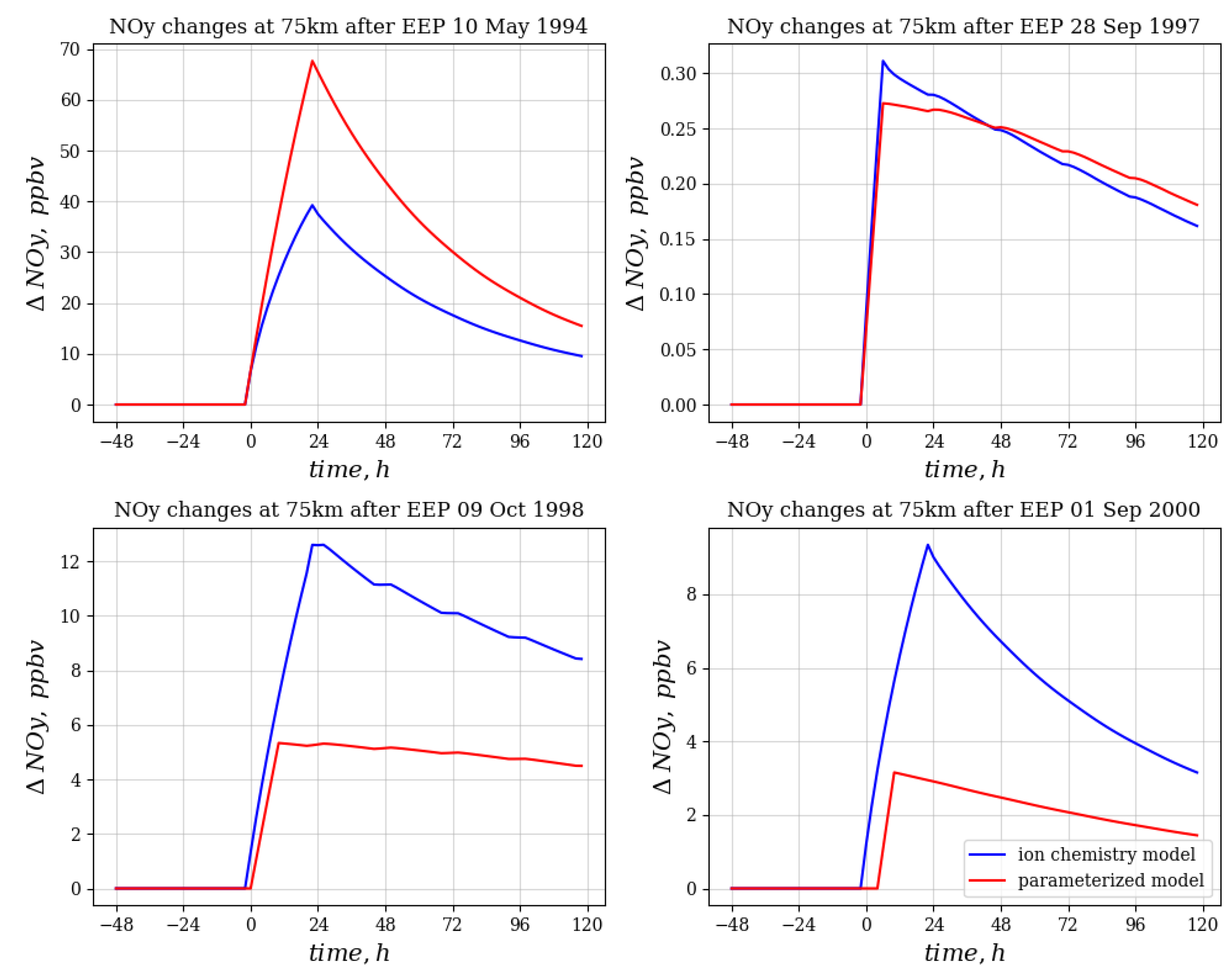
The effect of energetic electron precipitation on nitrogen oxides is observed for all four cases considered. However, the magnitude of the effect and the difference between versions of the model depend on the characteristics of the precipitation. The maximum effect (an increase in NOy by 40–70 ppbv) is observed for the 10 May 1994 event. Significantly less NOy response (3–13 ppbv) follows the events of 1 September 2000 and 9 October 2000, while the event of 28 September 1997 has a minimal effect. It is interesting to note that for weaker events, the parametrization underestimates the NOy response, while the opposite trend is observed for strong events. That can be explained by schemes of models: while the parameterized model takes into calculations simple fraction ratios, the full ion chemistry model affects wide branches of equations. Thus, the ion chemistry model is based not only on volume mixing ratios of species, but on chemical reactions of species as well. Additionally, it is seen that patterns of reduction of disturbances are different for events with long daylight hours: for events of 1 September and 10 May, reductions are exponential, while for events of 9 October and 28 September, decreases are approximately linear with stair-like patterns. These patterns are seen because the amount of sunlight is much less for these time periods.
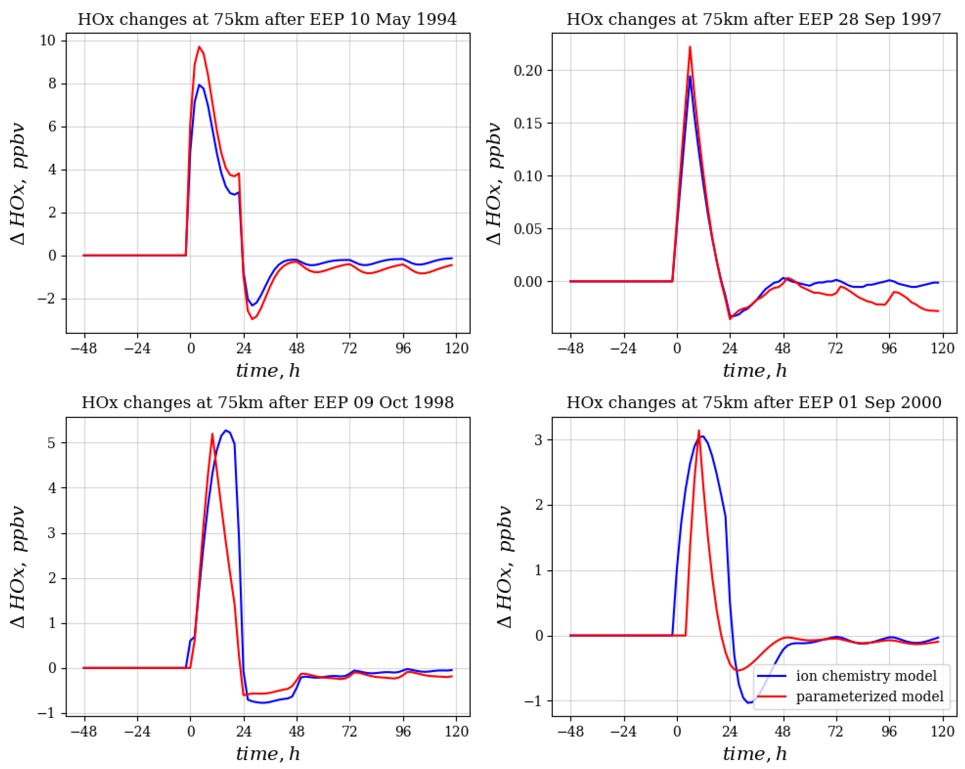
The response of hydrogen oxides shown in Figure 4 has similar features with respect to the magnitude of the effect. In this case, the event of 10 May 1994 dominates, and the effect reaches almost 10 ppbv. However, the parametrization used is in good agreement with the calculations using ion chemistry for all cases except for the weak event of 28 September 1997.
It is interesting to note a significant difference between the duration of periods with an increased content of the considered gases, which is related to their lifetime. Hydrogen oxides pass into a reservoir form almost within a day, while nitrogen oxides maintain an increased concentration for more than 5 days. However, the effect of longer-lived nitrogen oxides on the stratospheric ozone is not observed in the model due to the absence of intense downward currents and vertical diffusion in the period under consideration (May, September, October). By this reason, the stair-like patterns for HOx are not seen, but diurnal variations are denoted in Figure 4: the restored after disturbance volume mixing ratios of HOx are oscillating around zero value (under daytime HOx is reduced and during nighttime is produced).
Figure 5 shows the effect of EEP on the ozone for the events under consideration. As before, the strongest ozone drops (up to 30%) are observed on 10 May 1994, followed by the events of 9 October 1998 and 1 September 2000. On 28 September 1997, the decrease in ozone is very small (about 2% in the ion chemistry model).
The dependence of the degree of ozone depletion on the approach used to account for ionic chemistry is quite complex. In the case of a strong event, both approaches give approximately the same effect, which is explained by the dominant effect of hydrogen oxides on ozone. For moderate events, the ion chemistry variant gives a much stronger ozone drop. This can be explained either by the additional influence of nitrogen oxides or by the activation of chlorine oxides, which manifests itself for some time after the event only with a moderate increase in the NOy concentration. It is important that the model working with the use of parametrization is not able to take into account the impact of this kind, therefore, in further studies, it is planned to use the model with ion chemistry. Additionally, diurnal variations of ozone content are seen. During events of 9 October 1998 and 28 September 1997, these variations are observed: a day after the EEP impact saw that the ozone amount accumulates by midnight and dissipates after noon because of the sunlight presence. It is harder to observe such effect for the remaining two events because of longer daytime duration in May and beginning of September. In addition, we do observe the results of the enhanced catalytic HOx cycle [24,35]: there is an increase-decrease-increase pattern of ozone depletion, which is observed on the 10 May 1994 EEP event clearly.
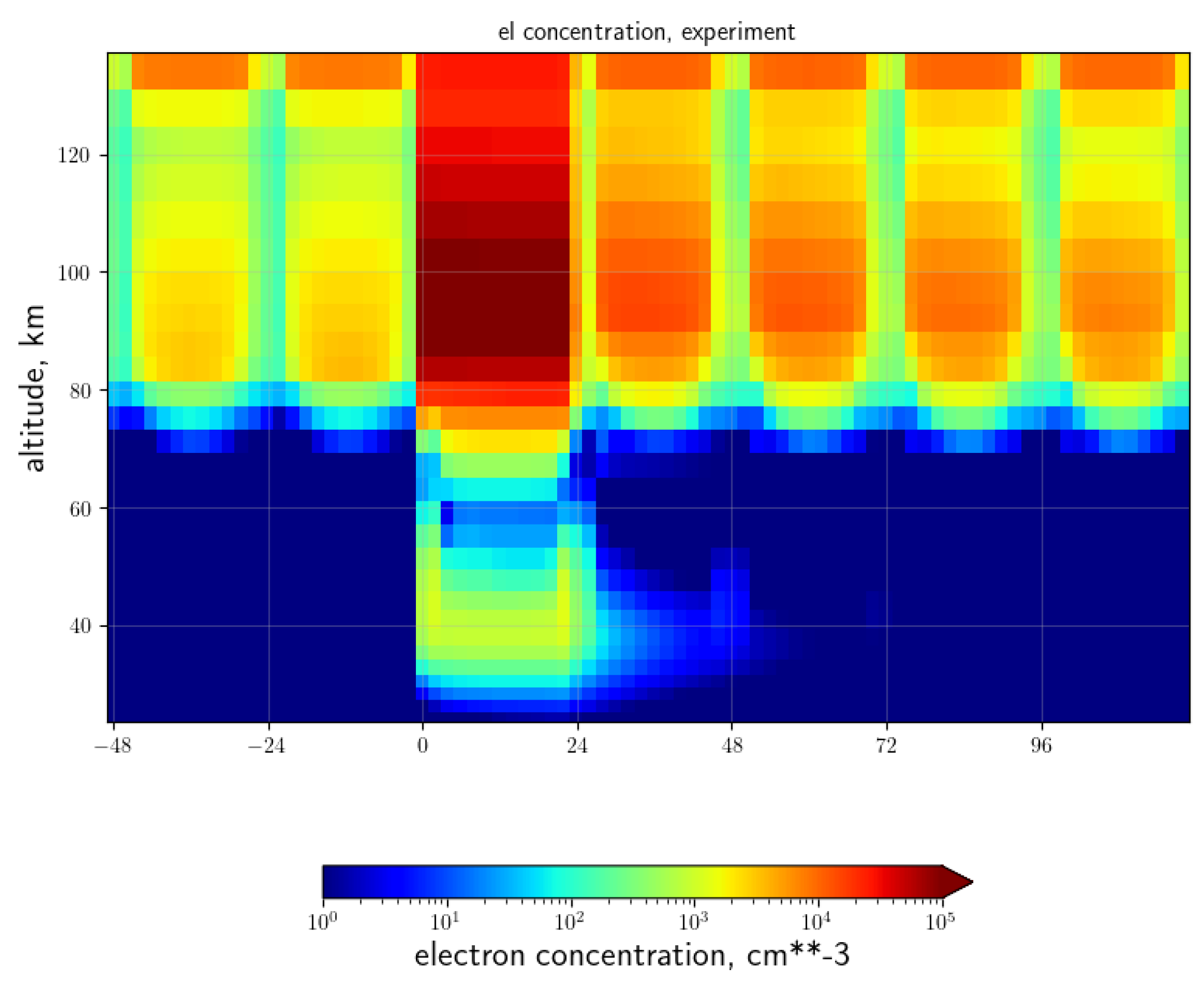
Figure 6 shows an example of the electron density induced by EEP and estimated by the model with interactive ion chemistry, taking into account information about EEP flux and spectra from balloon observations. Here, we observe that the electron concentration during geomagnetic disturbances reveals the D and E ionospheric layers. A strong increase in the electron concentration by two orders of magnitude at altitudes from about 30 to 120 km can be caused by EEP during geomagnetic disturbances with Kp = 4. Due to the efficient process of electron-ion recombination, after 24 h, the electron concentration returns to the normal form of the diurnal cycle after EEP forcing, which is clearly observed at altitudes above 80 km. At these altitudes, there is a change in the electron density: 103 electrons per cm3 before the EEP event, 105 electrons per cm3 during the EEP event. Then, there is a decrease in the increased concentration (reaches 104 electrons per cm3), which does not reach the concentration values before the event for 4 days. At altitudes below 80 km, a 24-h EEP effect is also defined. Although the increase in electron concentration is orders of magnitude greater than at upper altitudes, relaxation occurs much faster: the effect is noticeable only for 2 days.
As already mentioned in the introduction, the electron density above about 60 km can be observed with the help of radars and VLF transmitters, while below about 60 km, the electron density is not directly measured. Here, for the first time, an estimate of the electron density variability below about 60 km can be seen, based on actual balloon measurements that provided information on bremsstrahlung X-ray fluxes. Some numerical calculations of the electron density at the same heights based on synthetic EEP data limited by electron fluxes up to 1 MeV give order of magnitude lower values of the electron density, but the electron density calculated with EEP energy up to 10 MeV is the same order of magnitude as this is shown in Figure 6 [35]. Above about 60 km, electron density values are in good agreement with other calculations, e.g., [24,35] and, for example, EISCAT measurements, e.g., [15,24].
4. Discussions and Conclusions
The importance of understanding recent and predicting future changes in the ozone layer and climate, especially in the Arctic and subarctic, has important environmental, social, and economic implications. The urgency of the problem is exacerbated by the lack of strong evidence of the restoration of the ozone layer and the formation of ozone mini-holes. The study of the ozone layer requires taking into account the influence of natural and anthropogenic factors acting in the atmosphere from the Earth’s surface to near-Earth space.
One of the important natural factors that form the ozone layer is solar and geomagnetic activity and the associated processes of precipitation of energetic particles into the atmosphere. The role of energetic electrons precipitating from the radiation belts in ozone variations and climate change is still not clear, and additional studies are required to study the role of energetic electron precipitations (EEP) in ozone layer variations during geomagnetic disturbances.
The study of the behavior of region D of the high-latitude ionosphere under various geomagnetic conditions is necessary both in scientific and practical terms. The region D significantly affects the propagation of radio waves in a wide frequency range and temporal variations in the distribution of electron density determine complex amplitude and phase effects during their propagation. In recent years, the interest of specialists in various fields in the study of phenomena in the atmosphere of high latitudes has been growing. The reasons for this lie in the strategic position occupied by both the Arctic and Antarctic regions. The strong variability of the upper atmosphere of the polar region, associated with the complexity and diversity of the physical processes occurring there, creates difficulties today in predicting the parameters of radio communication, radio navigation, and other important characteristics in terms of application. This activates the study of the electron density over high latitudes during geomagnetic disturbances.
In this research, we take into account balloon observations of energetic electron precipitations of medium power in the polar high-latitude atmosphere over Apatity (L = 5.3) during geomagnetic disturbances characterized by Kp = 4. These observations made it possible to estimate the characteristic rates of atmospheric ionization and electron concentration as well as the destruction of mesospheric ozone.
After our study, we can conclude that the electron concentration can increase by two orders of magnitude over the altitudinal band from about 30 km to 120 km during geomagnetic disturbances.
It is shown that during geomagnetic disturbances, there is an increase in the concentration of reactive oxides of nitrogen and hydrogen relative to calm conditions, reaching significant values for intense EEP events. An increase in the concentration of radicals leads to the destruction of the ozone at the heights of the mesosphere during the day, with a maximum destruction of about 14 to 25% at a height of about 75 km for intense events. The effects obtained for events of medium intensity depend on the method of accounting for ion chemistry. In the case of high ionization rates, hydrogen oxides dominate, the growth of which models with equally reproduce parameterized and interactive ion chemistry. In the case of less intense events, the effect of an increase in nitrogen oxides and, probably, chlorine, which leads to more pronounced ozone depletion at an altitude of 75 km, is observed. It follows that the use of interactive ion chemistry leads to more interesting results. More accurate recommendations on the accuracy of the two methods used can only be made by comparison with observations. The influence of longer-lived nitrogen oxides on stratospheric ozone is not observed in the model due to the absence of intense downward currents in the period under consideration (May, September, October). Probably, this process will be more pronounced if EEP occurs during polar winter.
The obtained results can be used to better predict the future of the ozone and hazards layer as well as the state of the climate.
Author Contributions
Conceptualization: I.M. and G.B.; spectra and ionization rates computation: G.B. and I.M.; models simulations: D.G., E.R. and T.E.; validation and visualization: I.M. and D.G.; writing—original draft preparation: D.G., I.M., G.B. and E.R. All authors have read and agreed to the published version of the manuscript.
Funding
The EEP selection and ozone modeling was done by the RSF grant 22-62-00048, contract 1053-223-2022 “Atmospheric effects of precipitation of energetic electrons from the outer radiation belt: Part I”. Work on the prolongation models to 120 km was done under the RFBR project 20-05-00450. Investigation of electron density changes under EEP was done in the frame of the RFBR project 20-55-12020. This work was carried out at “Laboratory for the study of the ozone layer and the upper atmosphere” with the support of the Ministry of Science and Higher Education of the Russian Federation under agreement 075-15-2021-583.
Institutional Review Board Statement
Not applicable.
Informed Consent Statement
Not applicable.
Data Availability Statement
Kp index: https://kp.gfz-potsdam.de/en/data (accessed on 28 January 2023); EEP balloon observation data: https://sites.lebedev.ru/ru/DNS_FIAN/479.html (accessed on 28 January 2023). The models and data can be sent upon request.
Acknowledgments
We are thankful GFZ for the free data distribution. We are grateful to the reviewers for their careful reading of our manuscript and for their comments that helped to improve our article.
Conflicts of Interest
The authors declare no conflict of interest.
References
- Mironova, I.A.; Aplin, K.L.; Arnold, F.; Bazilevskaya, G.A.; Harrison, R.G.; Krivolutsky, A.A.; Nicoll, K.A.; Rozanov, E.V.; Turunen, E.; Usoskin, I.G. Energetic Particle Influence on the Earth’s Atmosphere. Space Sci. Rev. 2015, 194, 1–96. [Google Scholar] [CrossRef] [Green Version]
- Rozanov, E.V. Effect of Precipitating Energetic Particles on the Ozone Layer and Climate. Russ. J. Phys. Chem. B 2018, 12, 786–790. [Google Scholar] [CrossRef]
- Cooper, A.; Turney, C.S.M.; Palmer, J.; Hogg, A.; McGlone, M.; Wilmshurst, J.; Lorrey, A.M.; Heaton, T.J.; Russell, J.M.; McCracken, K.; et al. Response to Comment on “A Global Environmental Crisis 42,000 Years Ago”. Science 2021, 374, eabi9756. [Google Scholar] [CrossRef] [PubMed]
- Ball, W.T.; Alsing, J.; Mortlock, D.J.; Staehelin, J.; Haigh, J.D.; Peter, T.; Tummon, F.; Stübi, R.; Stenke, A.; Anderson, J.; et al. Evidence for a Continuous Decline in Lower Stratospheric Ozone Offsetting Ozone Layer Recovery. Atmos. Chem. Phys. 2018, 18, 1379–1394. [Google Scholar] [CrossRef] [Green Version]
- Witze, A. Rare Ozone Hole Opens over Arctic—and It’s Big. Nature 2020, 580, 18–19. [Google Scholar] [CrossRef] [Green Version]
- Timofeyev, Y.M.; Smyshlyaev, S.P.; Virolainen, Y.A.; Garkusha, A.S.; Polyakov, A.V.; Motsakov, M.A.; Kirner, O. Case Study of Ozone Anomalies over Northern Russia in the 2015/2016 Winter: Measurements and Numerical Modelling. Ann. Geophys. 2018, 36, 1495–1505. [Google Scholar] [CrossRef] [Green Version]
- Karagodin, A.; Mironova, I.; Artamonov, A.; Konstantinova, N. Response of the Total Ozone to Energetic Electron Precipitation Events. J. Atmos. Sol. Terr. Phys. 2018, 180, 153–158. [Google Scholar] [CrossRef] [Green Version]
- Szela̧g, M.E.; Marsh, D.R.; Verronen, P.T.; Seppälä, A.; Kalakoski, N. Ozone Impact from Solar Energetic Particles Cools the Polar Stratosphere. Nat. Commun. 2022, 13, 6883. [Google Scholar] [CrossRef] [PubMed]
- George, H.; Reeves, G.; Cunningham, G.; Kalliokoski, M.M.H.; Kilpua, E.; Osmane, A.; Henderson, M.G.; Morley, S.K.; Hoilijoki, S.; Palmroth, M. Contributions to Loss Across the Magnetopause During an Electron Dropout Event. J. Geophys. Res. Space Phys. 2022, 127, 751. [Google Scholar] [CrossRef]
- Wing, S.; Johnson, J.R.; Turner, D.L.; Ukhorskiy, A.Y.; Boyd, A.J. Untangling the Solar Wind and Magnetospheric Drivers of the Radiation Belt Electrons. J. Geophys. Res. Space Phys. 2022, 127, e2021JA030246. [Google Scholar] [CrossRef]
- Xu, W.; Marshall, R.A.; Tobiska, W.K. A Method for Calculating Atmospheric Radiation Produced by Relativistic Electron Precipitation. Space Weather 2021, 19, e2021SW002735. [Google Scholar] [CrossRef]
- Tobiska, W.K.; Didkovsky, L.; Judge, K.; Weiman, S.; Bouwer, D.; Bailey, J.; Atwell, B.; Maskrey, M.; Mertens, C.; Zheng, Y.; et al. Analytical Representations for Characterizing the Global Aviation Radiation Environment Based on Model and Measurement Databases. Space Weather 2018, 16, 1523–1538. [Google Scholar] [CrossRef] [PubMed]
- Millan, R.M.; McCarthy, M.P.; Sample, J.G.; Smith, D.M.; Thompson, L.D.; McGaw, D.G.; Woodger, L.A.; Hewitt, J.G.; Comess, M.D.; Yando, K.B.; et al. The Balloon Array for RBSP Relativistic Electron Losses (BARREL). Space Sci. Rev. 2013, 179, 503–530. [Google Scholar] [CrossRef] [Green Version]
- Woodger, L.A.; Halford, A.J.; Millan, R.M.; McCarthy, M.P.; Smith, D.M.; Bowers, G.S.; Sample, J.G.; Anderson, B.R.; Liang, X. A Summary of the BARREL Campaigns: Technique for Studying Electron Precipitation. J. Geophys. Res. Space Phys. 2015, 120, 4922–4935. [Google Scholar] [CrossRef] [PubMed]
- Miyoshi, Y.; Hosokawa, K.; Kurita, S.; Oyama, S.I.; Ogawa, Y.; Saito, S.; Shinohara, I.; Kero, A.; Turunen, E.; Verronen, P.T.; et al. Penetration of MeV Electrons into the Mesosphere Accompanying Pulsating Aurorae. Sci. Rep. 2021, 11, 13724. [Google Scholar] [CrossRef] [PubMed]
- Thomson, N.R.; Clilverd, M.A.; Rodger, C.J. Ionospheric D Region: VLF-Measured Electron Densities Compared With Rocket-Based FIRI-2018 Model. J. Geophys. Res. Space Phys. 2022, 127, e2022JA030977. [Google Scholar] [CrossRef]
- Mironova, I.; Bazilevskaya, G. Estimation of Characterized Ionization Rates during Geomagnetic Disturbances with Kp = 4 Based on Balloon Observations; Springer: Saint-Petersburg, Russia, 2023. [Google Scholar]
- Mironova, I.; Sinnhuber, M.; Bazilevskaya, G.; Clilverd, M.; Funke, B.; Makhmutov, V.; Rozanov, E.; Santee, M.L.; Sukhodolov, T.; Ulich, T. Exceptional Middle Latitude Electron Precipitation Detected by Balloon Observations: Implications for Atmospheric Composition. Atmos. Chem. Phys. 2022, 22, 6703–6716. [Google Scholar] [CrossRef]
- Mironova, I.; Kovaltsov, G.; Mishev, A.; Artamonov, A. Ionization in the Earth’s Atmosphere Due to Isotropic Energetic Electron Precipitation: Ion Production and Primary Electron Spectra. Remote Sens. 2021, 13, 4161. [Google Scholar] [CrossRef]
- Mironova, I.A.; Artamonov, A.A.; Bazilevskaya, G.A.; Rozanov, E.V.; Kovaltsov, G.A.; Makhmutov, V.S.; Mishev, A.L.; Karagodin, A.V. Ionization of the Polar Atmosphere by Energetic Electron Precipitation Retrieved From Balloon Measurements. Geophys. Res. Lett. 2019, 46, 990–996. [Google Scholar] [CrossRef] [Green Version]
- Artamonov, A.A.; Mishev, A.L.; Usoskin, I.G. Model CRAC:EPII for Atmospheric Ionization Due to Precipitating Electrons: Yield Function and Applications. J. Geophys. Res. Space Phys. 2016, 121, 1736–1743. [Google Scholar] [CrossRef]
- Mironova, I.; Bazilevskaya, G.; Kovaltsov, G.; Artamonov, A.; Rozanov, E.; Mishev, A.; Makhmutov, V.; Karagodin, A.; Golubenko, K. Spectra of High Energy Electron Precipitation and Atmospheric Ionization Rates Retrieval from Balloon Measurements. Sci. Total. Environ. 2019, 69, 133242. [Google Scholar] [CrossRef] [PubMed]
- Chaston, C.C.; Bonnell, J.W.; Halford, A.J.; Reeves, G.D.; Baker, D.N.; Kletzing, C.A.; Wygant, J.R. Pitch Angle Scattering and Loss of Radiation Belt Electrons in Broadband Electromagnetic Waves. Geophys. Res. Lett. 2018, 45, 9344–9352. [Google Scholar] [CrossRef]
- Turunen, E.; Kero, A.; Verronen, P.T.; Miyoshi, Y.; Oyama, S.I.; Saito, S. Mesospheric Ozone Destruction by High-Energy Electron Precipitation Associated with Pulsating Aurora. J. Geophys. Res. 2016, 121, 11852–11861. [Google Scholar] [CrossRef]
- Matthes, K.; Funke, B.; Andersson, M.E.; Barnard, L.; Beer, J.; Charbonneau, P.; Clilverd, M.A.; Dudok De Wit, T.; Haberreiter, M.; Hendry, A.; et al. Solar Forcing for CMIP6 (v3.2). Geosci. Model. Dev. 2017, 10, 2247–2302. [Google Scholar] [CrossRef] [Green Version]
- Stozhkov, Y.I.; Svirzhevsky, N.S.; Bazilevskaya, G.A.; Kvashnin, A.N.; Makhmutov, V.S.; Svirzhevskaya, A.K. Long-Term (50 Years) Measurements of Cosmic Ray Fluxes in the Atmosphere. Adv. Space Res. 2009, 44, 1124–1137. [Google Scholar] [CrossRef]
- Makhmutov, V.S.; Bazilevskaya, G.A.; Stozhkov, Y.I.; Svirzhevskaya, A.K.; Svirzhevsky, N.S. Catalogue of Electron Precipitation Events as Observed in the Long-Duration Cosmic Ray Balloon Experiment. J. Atmos. Sol. Terr. Phys. 2016, 149, 258–276. [Google Scholar] [CrossRef]
- Bazilevskaya, G.A.; Kalinin, M.S.; Krainev, M.B.; Makhmutov, V.S.; Stozhkov, Y.I.; Svirzhevskaya, A.K.; Svirzhevsky, N.S.; Gvozdevsky, B.B. Temporal Characteristics of Energetic Magnetospheric Electron Precipitation as Observed During Long-Term Balloon Observations. J. Geophys. Res. Space Phys. 2020, 125, e2020JA028033. [Google Scholar] [CrossRef]
- Bernhardt, P.A.; Hua, M.; Bortnik, J.; Ma, Q.; Verronen, P.T.; McCarthy, M.P.; Hampton, D.L.; Golkowski, M.; Cohen, M.B.; Richardson, D.K.; et al. Active Precipitation of Radiation Belt Electrons Using Rocket Exhaust Driven Amplification (REDA) of Man-Made Whistlers. J. Geophys. Res. Space Phys. 2022, 127, e2022JA030358. [Google Scholar] [CrossRef]
- Direct Access to POES SEM Data. Available online: https://www.ngdc.noaa.gov/stp/satellite/poes/dataaccess.html (accessed on 28 January 2022).
- Porter, H.S.; Jackman, C.H.; Green, A.E.S. Efficiencies for Production of Atomic Nitrogen and Oxygen by Relativistic Proton Impact in Air. J. Chem. Phys. 1976, 65, 154–167. [Google Scholar] [CrossRef]
- Sinnhuber, M.; Nieder, H.; Wieters, N. Energetic Particle Precipitation and the Chemistry of the Mesosphere/Lower Thermosphere. Surv. Geophys. 2012, 33, 1281–1334. [Google Scholar] [CrossRef]
- Solomon, S.; Rusch, D.W.; Gitrard, J.-C.; Red, G.C.; Crutzenk, P.J. The Effect Neutral and of Particle Precipitation Events on the Ion Chemistry of the Middle Atmosphere: II. Odd Hydrogen. Planet. Space Sci. 1981, 29, 885–893. [Google Scholar] [CrossRef]
- Verronen, P.T.; Andersson, M.E.; Marsh, D.R.; Kovács, T.; Plane, J.M.C. WACCM-D Whole Atmosphere Community Climate Model with D-Region Ion Chemistry. J. Adv. Model. Earth Syst. 2016, 8, 954–975. [Google Scholar] [CrossRef]
- Xu, W.; Marshall, R.A.; Fang, X.; Turunen, E.; Kero, A. On the Effects of Bremsstrahlung Radiation During Energetic Electron Precipitation. Geophys. Res. Lett. 2018, 45, 1167–1176. [Google Scholar] [CrossRef]
Figure 1.
Upper panel: Energy spectra of precipitating energetic electrons obtained from balloon observations. Low panel: Altitude profiles of the ionization rates over Apatity (67.57 N, 33.56 E, L = 5.3) during geomagnetic disturbances with Kp = 4.
Figure 1.
Upper panel: Energy spectra of precipitating energetic electrons obtained from balloon observations. Low panel: Altitude profiles of the ionization rates over Apatity (67.57 N, 33.56 E, L = 5.3) during geomagnetic disturbances with Kp = 4.

Figure 2.
Ozone changes after EEP. The 0 on the horizontal axis is midnight of 10 May 1994.

Figure 3.
Simulation results of NOy change at 75 km. The 0 on the horizontal scale is midnight of the corresponding day.
Figure 3.
Simulation results of NOy change at 75 km. The 0 on the horizontal scale is midnight of the corresponding day.

Figure 4.
Simulation results of HOx change at 75 km. The 0 on the horizontal scale is midnight of the corresponding day.
Figure 4.
Simulation results of HOx change at 75 km. The 0 on the horizontal scale is midnight of the corresponding day.

Figure 5.
Simulation results of ozone change at 75 km. The 0 on the horizontal scale is midnight of the corresponding day.
Figure 5.
Simulation results of ozone change at 75 km. The 0 on the horizontal scale is midnight of the corresponding day.

Figure 6.
Simulation results of electron density before and after EEP on 28 September 1997.


Table 1.
Day of the year (DOY) and time of balloon observations, EEP spectra parameters, intensity of geomagnetic disturbances on these days.
Table 1.
Day of the year (DOY) and time of balloon observations, EEP spectra parameters, intensity of geomagnetic disturbances on these days.
| Date (DOY) | Start Time (UT) –End Time (UT) | Spectra Parameters Kp (UT) F0 k |
|---|---|---|
| 10 May 1994 (129) | 7 h 10 m–7 h 58 m | 1.94 × 10¹³ 4.62 4 (00–21 h) |
| 28 Sep. 1997 (270) | 7 h 00 m–7 h 32 m | 6.29 × 10¹⁶ 7.14 4 (00–06 h) |
| 9 Oct. 1998 (281) | 7 h 48 m–8 h 16 m | 5.48 × 10¹⁵ 6.09 4 (03–09 h) |
| 1 Sep. 2000 (245) | 7 h 42 m–8 h 37 m | 8.68 × 10¹¹ 3.97 4 (06–09 h) |
Disclaimer/Publisher’s Note: The statements, opinions and data contained in all publications are solely those of the individual author(s) and contributor(s) and not of MDPI and/or the editor(s). MDPI and/or the editor(s) disclaim responsibility for any injury to people or property resulting from any ideas, methods, instructions or products referred to in the content. |
© 2023 by the authors. Licensee MDPI, Basel, Switzerland. This article is an open access article distributed under the terms and conditions of the Creative Commons Attribution (CC BY) license (https://creativecommons.org/licenses/by/4.0/).
Share and Cite
MDPI and ACS Style
Grankin, D.; Mironova, I.; Bazilevskaya, G.; Rozanov, E.; Egorova, T. Atmospheric Response to EEP during Geomagnetic Disturbances. Atmosphere 2023, 14, 273. https://doi.org/10.3390/atmos14020273
AMA Style
Grankin D, Mironova I, Bazilevskaya G, Rozanov E, Egorova T. Atmospheric Response to EEP during Geomagnetic Disturbances. Atmosphere. 2023; 14(2):273. https://doi.org/10.3390/atmos14020273
Chicago/Turabian StyleGrankin, Dmitry, Irina Mironova, Galina Bazilevskaya, Eugene Rozanov, and Tatiana Egorova. 2023. "Atmospheric Response to EEP during Geomagnetic Disturbances" Atmosphere 14, no. 2: 273. https://doi.org/10.3390/atmos14020273
Note that from the first issue of 2016, this journal uses article numbers instead of page numbers. See further details here.