Updating and Evaluating Anthropogenic Emissions for NOAA’s Global Ensemble Forecast Systems for Aerosols (GEFS-Aerosols): Application of an SO₂ Bias-Scaling Method

Abstract

We updated the anthropogenic emissions inventory in NOAA’s operational Global Ensemble Forecast for Aerosols (GEFS-Aerosols) to improve the model’s prediction of aerosol optical depth (AOD). We used a methodology to quickly update the pivotal global anthropogenic sulfur dioxide (SO₂) emissions using a speciated AOD bias-scaling method. The AOD bias-scaling method is based on the latest model predictions compared to NASA’s Modern-Era Retrospective analysis for Research and Applications, version 2 (MERRA2). The model bias was subsequently applied to the CEDS 2019 SO₂ emissions for adjustment. The monthly mean GEFS-Aerosols AOD predictions were evaluated against a suite of satellite observations (e.g., MISR, VIIRS, and MODIS), ground-based AERONET observations, and the International Cooperative for Aerosol Prediction (ICAP) ensemble results. The results show that transitioning from CEDS 2014 to CEDS 2019 emissions data led to a significant improvement in the operational GEFS-Aerosols model performance, and applying the bias-scaled SO₂ emissions could further improve global AOD distributions. The biases of the simulated AODs against the observed AODs varied with observation type and seasons by a factor of 3~13 and 2~10, respectively. The global AOD distributions showed that the differences in the simulations against ICAP, MISR, VIIRS, and MODIS were the largest in March–May (MAM) and the smallest in December–February (DJF). When evaluating against the ground-truth AERONET data, the bias-scaling methods improved the global seasonal correlation (r), Index of Agreement (IOA), and mean biases, except for the MAM season, when the negative regional biases were exacerbated compared to the positive regional biases. The effect of bias-scaling had the most beneficial impact on model performance in the regions dominated by anthropogenic emissions, such as East Asia. However, it showed less improvement in other areas impacted by the greater relative transport of natural emissions sources, such as India. The accuracies of the reference observation or assimilation data for the adjusted inputs and the model physics for outputs, and the selection of regions with less seasonal emissions of natural aerosols determine the success of the bias-scaling methods. A companion study on emission scaling of anthropogenic absorbing aerosols needs further improved aerosol prediction.

1. Introduction

Anthropogenic emissions in the atmosphere result from human activities such as energy production and consumption, crop and livestock production, and land-use changes. Key anthropogenic emission sectors include electricity production, industrial activities, residential cooking and heating, and transportation. There are two main methods of producing anthropogenic emissions, bottom-up methods, based on the activity data together with sector-, fuel-, and species-specific emission factors, and top-down methods, inversely estimating emissions from the observed air pollutant concentrations [1,2,3,4]. Bottom-up methods can provide detailed estimates by the fuel and the sector, long-term trends, and, in many cases, emissions from specific facilities [2,3,4]. Top-down methods, which often are constructed by combining observational data and chemical transport models, can potentially point to emissions missed or overestimated by bottom-up approaches and provide more up-to-date information on the evolution of anthropogenic emissions [2,3,4]. In any case, building emission inventories require a significant amount of time, effort, and data collection and processing, which means that the emission data used in global aerosol and atmospheric composition (AAC) models generally lag a few years behind the present.

There are numerous global anthropogenic emission datasets that are publicly available, which include the Hemispheric Transport of Air Pollution (HTAP v2) [5] from 2008 to 2010 and HTAP v3, extending from 2000 to 2018 [5]; the Emissions Database for Global Atmospheric Research (EDGAR) [6] from 1970 to 2018; Evaluating the Climate and Air Quality Impacts of Short-Lived Pollutants (ECLIPSE) [7] from 1990 to 2010; and the Community Emission Data Systems (CEDS) [8,9], which currently extends from 1750 to 2019 (data are available in [10]). Such global anthropogenic emissions inventories include sector- and region-specific emissions data of gases and aerosols collected by a bottom-up method. Among them, the CEDS has historically been one of the most widely used inventories in the current suite of global AAC models (e.g., NASA GOCART, Harvard GEOS-Chem, and CMIP6).

Emissions data are essential inputs in simulating air quality and Earth system processes. However, applying existing emission data may not work ad hoc, as human activities can rapidly change in response to environmental, political, and economic factors. For example, during the recent COVID-19 pandemic, there were profound and widespread decreases in anthropogenic emissions, which led to both increases and decreases in anthropogenic pollutant concentrations [11,12,13,14,15,16,17,18,19,20,21,22]. Continuous measurements by satellite instruments can provide important information to rapidly update outdated bottom-up emissions inventories during such cases as the COVID-19 economic slowdown and be further used in global AAC models to quantify the impacts on air quality [18]. Furthermore, the use of data assimilation techniques for both chemical concentrations [23] and emissions (in conjunction with inverse modeling, as shown in [24]) can also improve AAC model predictions when input emissions datasets lag behind the forecast/simulated period or potentially contain biases.

This study aims to update the anthropogenic emissions data in a global AAC modeling system and evaluate the impact on predicted 3D aerosol concentrations. Using an aerosol optical depth (AOD) reanalysis dataset, we apply an AOD bias-scaling approach to update the emissions further and evaluate the impact on ACC-predicted aerosol concentrations. Here, we use the NOAA’s Global Ensemble Forecast System with aerosols (GEFS-Aerosols; [25]) that has adopted the Goddard Chemistry Aerosol Radiation and Transport (GOCART; [26]) modules to perform the emissions update and evaluate the forecasted aerosol concentrations and compute the aerosol optical depth (AOD).

The rapid bias-scaling method is based on a global reanalysis dataset to update the CEDS anthropogenic SO₂ emissions data across different regions. We assume that SO₂ emissions have a pseudo-linear relationship with sulfate AOD. The global average sulfate AOD at 500 nm corresponds to almost two thirds of anthropogenic AODs, which are the sum of sulfate, organic carbon (OC), and black carbon (BC) [26]. About 75~80% of the sulfate precursor emissions are from anthropogenic sources, which contribute 67% to the total sulfate burden [27]. We derive the monthly SO₂ emission scaling factor from ratios of the changes in SO₂ emissions to the difference in sulfate AODs between the Modern-Era Retrospective analysis for Research and Applications, version 2 (MERRA2) [28] and GEFS-Aerosols. Then, we update the SO₂ emission data closer to the GEFS-Aerosols near-real-time (NRT) forecasting time and predict the distributions of aerosol concentrations in 2021.

The objective of this study is to investigate the effects of the SO₂ bias-scaling methods on GEFS-Aerosols predictions in terms of the responsiveness to the observed AODs. Before updating anthropogenic SO₂ emissions, we look at the distributions of the existing emissions, such as CEDS 2014 and CEDS 2019, and the features of SO₂ emissions change from 2014 to 2019 (Section 2). We compare the GEFS-Aerosols-modeled AOD to different observations and ensemble simulation data and analyze the global and regional effects of bias-scaled SO₂ emissions on GEDS-Aerosol’s AOD. We discuss the regions where the updated emissions effectively improve model performances, particularly regarding the changes linked to seasonal SO₂ emission scaling (Section 3). We also present the implications and utility of this study. Finally, we discuss the limitations of the bias-scaling method and how this may be improved further for NRT aerosol prediction (Section 4 and Section 5).

2. Methods

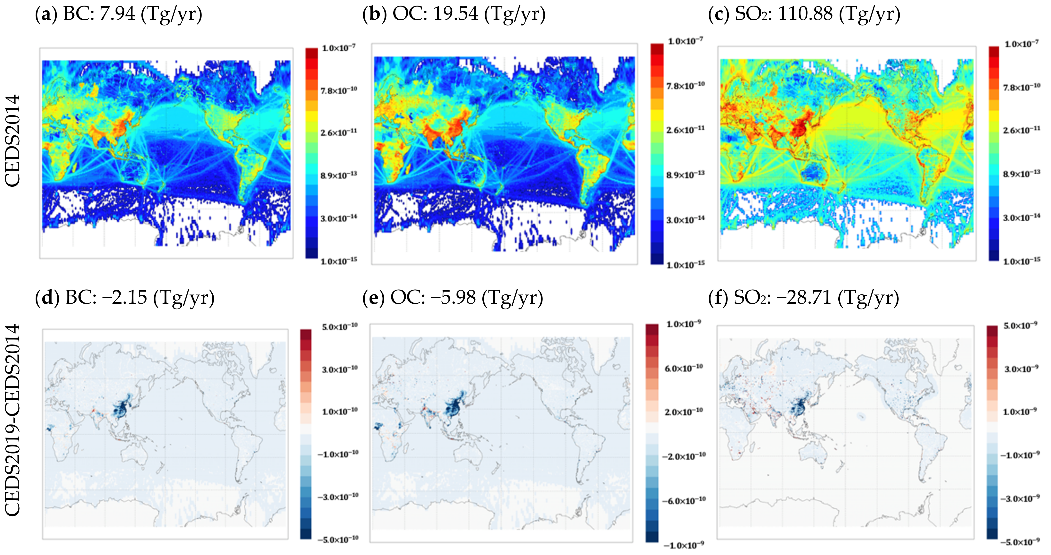
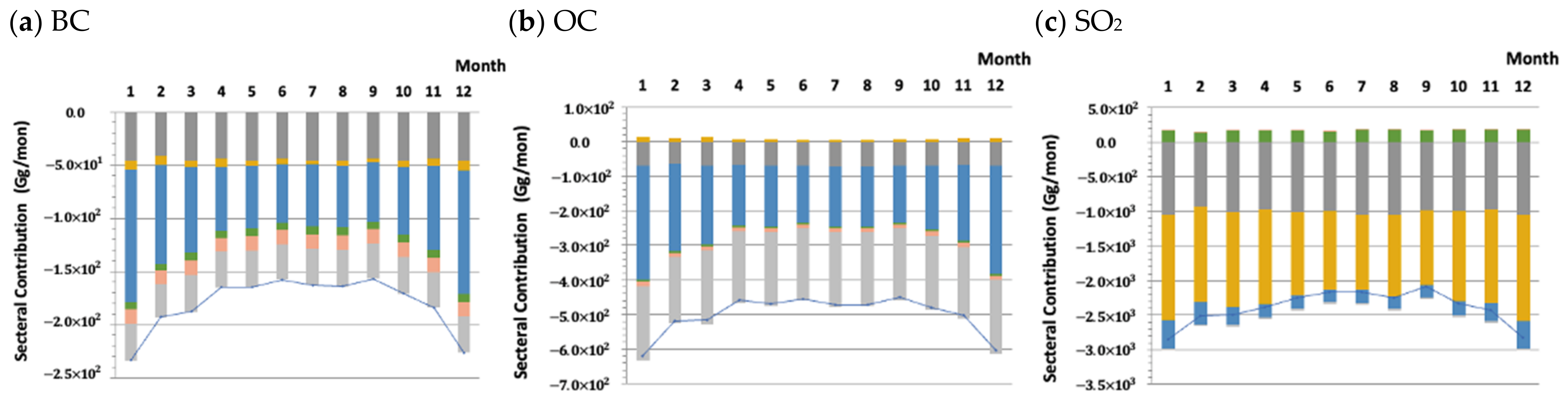
2.1. Emission Data: CEDS 2014 and CEDS 2019

This study uses CEDS 2014 [8] and CEDS 2019 [9] data for SO₂, BC, and OC emissions, and HTAPv2.2 2010 [5] for the unspeciated PM2.5 emissions used in the GOCART model for an experimental version of NOAA’s GEFS-Aerosol system used in this work.

CEDS 2014 is a collection of historical emission datasets (from 1750 to 2014) of anthropogenic reactive gases, greenhouse gases (GHG), and carbonaceous aerosols. CEDS produces a consistent emission time series based on the energy statistics from the International Energy Agency (IEA) and default emissions from EDGAR and GAINS, while scaling to match authoritative country-level inventories for recent years. It is arranged in a gridded form with monthly seasonality on an annual basis at the country and sector levels. CEDS estimates are generally slightly higher than the Coupled Model Intercomparison Project Phase 5 (CMIP 5) [29], EDGAR, and ECLIPSE estimates. CEDS 2019 updates CEDS 2014 by extending the emissions estimated from 2014 to 2019 [9]. Global estimates of NO_x, CO, SO₂, NH₃, non-methane volatile organic compounds (NMVOCs), BC, and OC over time are created as a function of eleven sectors and four fuel categories. They include monthly gridded (0.1° × 0.1°) emission fluxes using activity data for combustion- and process-level emission sources. CEDS 2019 results in lower emissions than CEDS 2014 for all compounds, except NMVOCs in Africa and BC in India. The uncertainties in the emissions of SO₂ are the smallest, and those of NH₃, OC, and BC are larger than the other species. Henceforth, we use “CEDS 2014” to refer to 2014 emission values from the CEDS 2014 data and “CEDS 2019” to refer to 2019 values from the CEDS 2019 data.

The HTAP v2.2 emission database is a mosaic grid map for SO₂, NO_x, CO, NMVOC, NH₃, PM10, PM2.5, and BC and OC aerosols for the years 2008 and 2010, after compiling regional inventories such as the United States Environmental Protection Agency (EPA) and Environment Canada for North America, European Monitoring and Evaluation Program–Netherlands Organization for Applied Scientific Research (EMAP-TNO) for Europe, Model Intercomparison Study (MICS) for Asia, and the EDGAR v 4.3 database for the rest of the world. This provides comprehensive and consistent monthly, global, sector-specific grid information on the emission of air pollutants for global and regional scale modeling [5].

The global distributions of BC, OC, and SO₂ are compared in CEDS 2014, as well as their differences from CEDS 2019 (Figure 1). The global emission amounts of the three species are different; however, their spatial emission patterns are very similar. East Asia, India, and Europe are the main areas of high emissions. The differences in BC, OC, and SO₂ emissions between CEDS 2014 and CEDS 2019 are 27.09%, 30.60%, and 25.90%, respectively.

Figure 2 shows the monthly distributions of the differences in the sectoral emissions of BC, OC, and SO₂ between CEDS 2014 and CEDS 2019. There are eight sectors, which are as follows: agriculture (AGR), energy (ENE), industry (IND), residential–commercial–others (RCO), international shipping (SHP), solvent-production applications (SLV), road transportation (TRA), and waste (WST). The RCO, ENE, and WST sectors differ significantly in terms of BC and OC emissions. The ENE (including fossil production and electricity generation) and IND (including fuel combustion and process emissions, such as smelting) sectors are the most significant contributors to SO₂ emissions. In terms of changes from CEDS 2014 to CEDS 2019, the largest sectors for BC, OC, and SO₂ are found in the RCO, RCO/WST, and IND sectors, respectively.

The global distributions of sectoral emissions of SO₂ for CEDS 2014 (Figure 3) show that the top three emission sectors, ENE, IND, and RCO, are the strongest in East Asia, and then the northeast border of India, along with the Himalayan mountains, Saudi Arabia, and Western Europe. The SO₂ emissions in CEDS 2019 increased in the SHP sector, compared to CEDS 2014, which are dominant along the coasts of large cities.

2.2. Model Configuration and Experimental Design

The GEFS-Aerosols model used in this study is one ensemble member of GEFS [25]. GEFS comprises 31 ensemble members, each containing a weather-forecast model at a horizontal resolution of about 25 km, with 64 vertical layers from the surface to 0.2 hPa. The GEFS is constructed with the Finite Volume-Cubed Sphere (FV3), non-hydrostatic dynamical core [30], and physics package based on NOAA’s Global Forecast System (GFS), version 15 (GFS v15) ([31,32],

Table 1. Simulation set-ups with emissions data.

Run	Emissions System	Anthropogenic Inventory
		SO2	BC	OC	PM2.5
BASE	NEXUS	CEDS 2014	CEDS 2014	CEDS 2014	HTAP 2010
SENS1	NEXUS	CEDS 2019 (unscaled)	CEDS 2019	CEDS 2019	HTAP 2010
SENS2	NEXUS	CEDS 2019 (scaled)	CEDS 2019	CEDS 2019	HTAP 2010
Simulation Periods: January–December 2021

).

To prepare the model-ready emissions for GEFS-Aerosol, we use the NOAA Emission and eXchange Unified System (NEXUS, [33,34]). NEXUS is an emission-modeling system based on the Harvard-NASA Emission Component (HEMCO [35]), a stand-alone software component for computing emissions in global atmospheric models. The HEMCO core acts as a compiler between raw emission datasets and targeted atmospheric models and creates a specific configuration in space and time.

CEDS 2014 and 2019 were used for the simulation design for SO₂, BC, and OC in BASE and SENS1, respectively (Table 1). HTAP v2.2 was used for the remaining un-speciated PM2.5 emissions in GEFS-Aerosol BASE and SENS1 simulations. SENS2 was simulated with the application of the AOD bias-scaling method to the SO₂ emissions of CEDS 2019 (see Section 2.3 below). The simulation period includes a full calendar year for 2021.

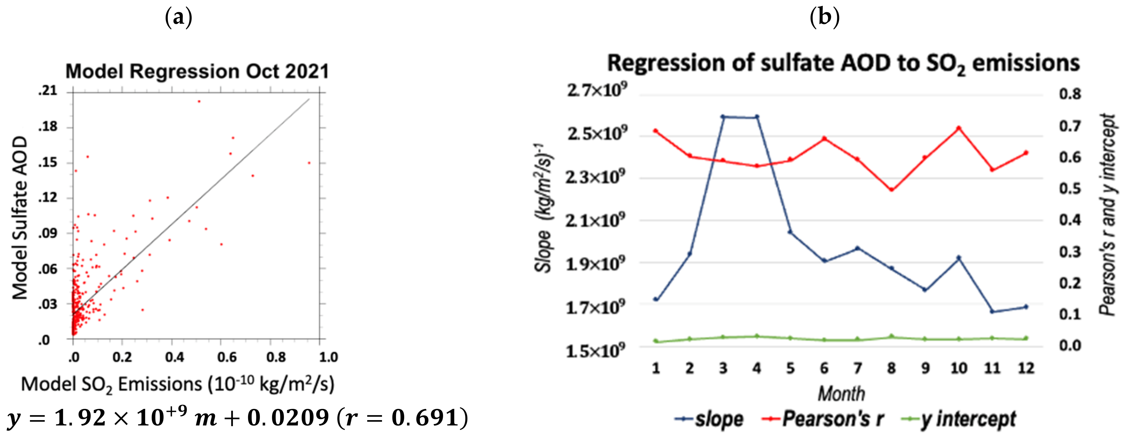
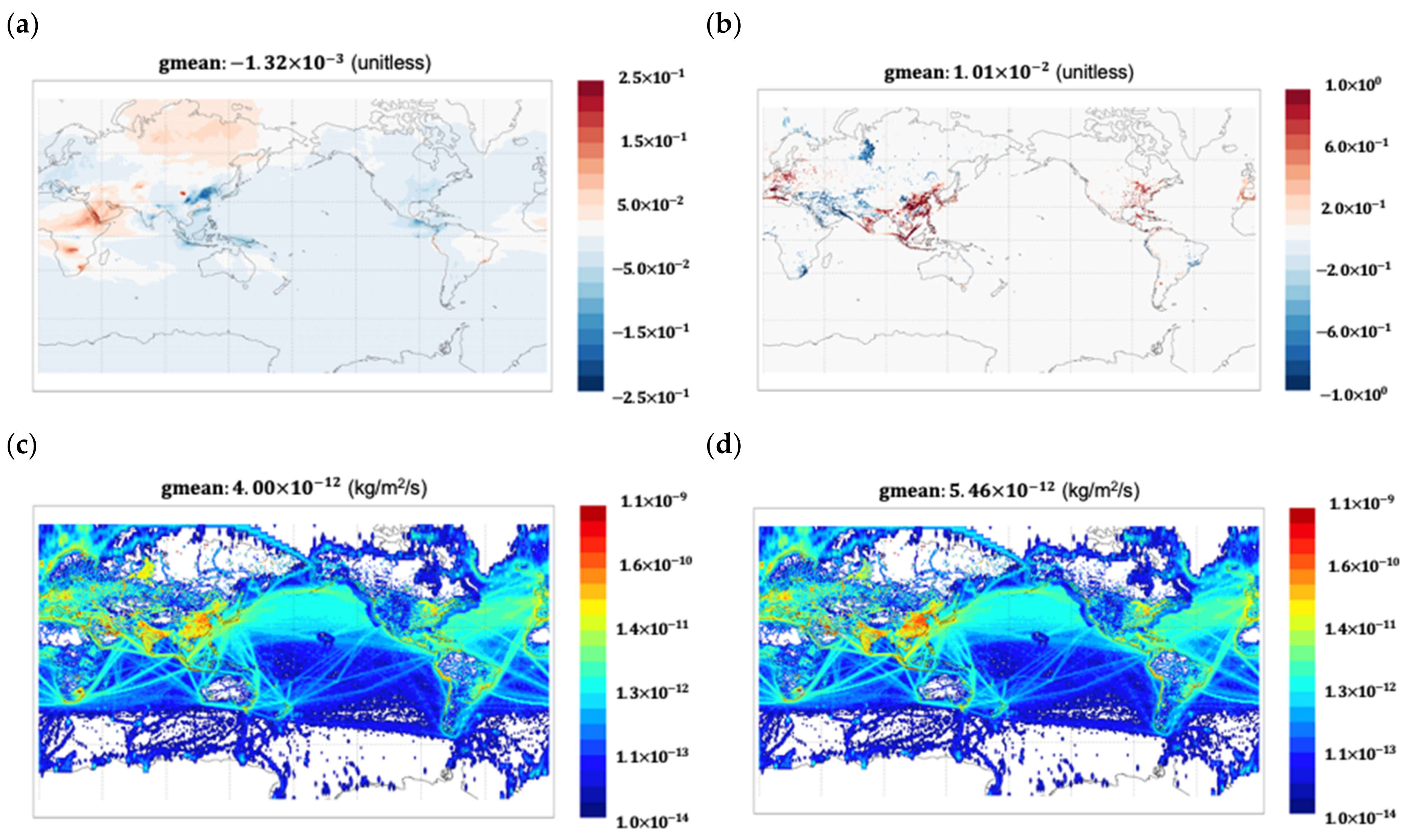
2.3. Bias-Scaling Methods

The bias-scaling method in this work is based on an approximately linear relationship between SO₂ gas emissions inputs and the GEFS-Aerosol-predicted AOD for sulfate (sulfate AOD). The AOD is calculated by integrating the product of the aerosol extinction coefficient and aerosol loading from the top of the atmosphere to the surface.

$${\mathsf{{\rm T}}}_{\mathrm{ext} \mathrm{at} 550\mathrm{nm}}={{\displaystyle \int }}_{\mathrm{TOA}}^{\mathrm{sfc}}{\mathsf{\sigma }}_{\mathrm{ext} \mathrm{at} 550\mathrm{nm}}\mathrm{ds}={{\displaystyle \int }}_{\mathrm{TOA}}^{\mathrm{sfc}}{\mathsf{\sigma }}_{\mathrm{ext} \mathrm{at} 550\mathrm{nm}} \ast \mathrm{C}\_\mathrm{aer} \mathrm{dz}$$

(1)

where ${\mathsf{\tau }}_{\mathrm{ext} \mathrm{at} 550\mathrm{nm}}$ is the extinction AOD at 550 nm. ${\mathsf{\Sigma }}_{\mathrm{ext} \mathrm{at} 550\mathrm{nm}}$ is the aerosol mass extinction coefficient (m²/g). $\mathrm{C}\_\mathrm{aer}$ is the aerosol mass concentration (kg/m³). $\mathrm{Ds}$ is the aerosol path length (kg/m²), and $\mathrm{dz}$ is the atmospheric thickness (m). Thus, the AOD is proportional to the aerosol concentration, and its relationships with precursor anthropogenic gas emissions ($\mathsf{\epsilon }$) can be derived for some species.

First, a high-to-low resolution, regional-scale filter (12° × 6°) is applied to the model outputs and emissions data for the regression analysis. Figure 4 shows the regression of GEFS-Aerosol-predicted AOD sulfate against its original input SO₂ emissions (${\mathsf{\epsilon }}_{\mathrm{SO}2\_\mathrm{gefs}}$) for October 2021. Here, we note a good regional correlation (Pearson correlation coefficient: ~0.7) between the input SO₂ emissions and GEFS-Aerosol-predicted AOD (Figure 4). Thus, assuming that the monthly average anthropogenic SO₂ emissions are the dominant source for the monthly average GEFS-Aerosol-predicted sulfate AOD, we use the regression analysis to determine a simple emissions bias-scaling factor for each month of the 2021 SENS1 simulation.

The slope, m, is calculated by the differences in the predicted sulfate AOD ($\Delta {\mathrm{AOD}}_{\mathrm{sulf}\_\mathrm{gefs}}$) over the differences in the input CEDS 2019 SO₂ emissions ($\Delta {\mathsf{\epsilon }}_{\mathrm{So}2\_\mathrm{gefs}}$).

$$\mathrm{m}=\frac{\Delta {\mathrm{AOD}}_{\mathrm{sulf}\_\mathrm{gefs}}}{\Delta {\mathsf{\epsilon }}_{\mathrm{SO}2\_\mathrm{gefs}}}$$

(2)

Then, the change in GEFS-Aerosol input SO₂ emissions ($\Delta {\mathsf{\epsilon }}_{\mathrm{SO}2\_\mathrm{gefs}}$) is obtained by dividing the difference in the sulfate AOD between GEFS-Aerosol and MERRA2 $({\mathrm{AOD}}_{\mathrm{sulfate}\_\mathrm{gefs}}-{\mathrm{AOD}}_{\mathrm{sulfate}\_\mathrm{merra}2}$) by the slope of the regression, m.

$$\Delta {\mathsf{\epsilon }}_{\mathrm{SO}2\_\mathrm{gefs}}=\frac{{\mathrm{AOD}}_{\mathrm{sulfate}\_\mathrm{gefs}}-{\mathrm{AOD}}_{\mathrm{sulfate}\_\mathrm{merra}2}}{\mathrm{m}}$$

(3)

where the SO₂ emissions scaling factor, $x$, is determined by dividing the sum of the $\Delta {\mathsf{\epsilon }}_{\mathrm{SO}{2}_{\mathrm{gefs}}}$ and the original CEDS 2019 SO₂ emissions (${\mathsf{\epsilon }}_{\mathrm{SO}{2}_{\mathrm{gefs}}}$) by ${\mathsf{\epsilon }}_{\mathrm{So}{2}_{\mathrm{gefs}}}$.

$$\mathrm{X}=\frac{\Delta {\mathsf{\epsilon }}_{\mathrm{SO}{2}_{\mathrm{gefs}}}+{ \mathsf{\epsilon }}_{\mathrm{SO}{2}_{\mathrm{gefs}}}}{{\mathsf{\epsilon }}_{\mathrm{SO}{2}_{\mathrm{gefs}}}}$$

(4)

Finally, the updated CEDS 2019 SO₂ emissions used in the model, ${\mathsf{\epsilon }}_{\mathrm{SO}2\_\mathrm{model}}$, are determined by multiplying the original ${\mathsf{\epsilon }}_{\mathrm{SO}{2}_{\mathrm{gefs}}}$ by the scaling factor, $x$.

$${\mathsf{{\rm E}}}_{\mathrm{SO}2\_\mathrm{model}} = x \times {\mathsf{\epsilon }}_{\mathrm{SO}{2}_{\mathrm{gefs}}}$$

(5)

We also applied a threshold criterion to scale only major SO₂ emissions sources (>1 $\times$ 10⁻¹¹ kg m⁻² s⁻¹). We noted that in some regions, the AOD sulfate bias (GEFS-MERRA2) change could be largely negative over certain regions, with relatively low ${\mathsf{\epsilon }}_{\mathrm{SO}{2}_{\mathrm{gefs}}}$, and thus result in unphysical negative emissions. In this case, we set an arbitrarily low bottom threshold of $\Delta {\mathsf{\epsilon }}_{\mathrm{SO}{2}_{\mathrm{gefs}}} as$1 $\times$ 10⁻²⁵ kg m⁻² s⁻¹ to remove such artificial negative emissions. Furthermore, we also applied a threshold criterion to scale only the largest SO₂ emission sources (>1 $\times$ 10⁻¹¹ kg m⁻² s⁻¹). To check for overfitting in our linear regression analysis, we used the mean square errors (MSEs) of SENS1 and SENS2 against MERRA2 AOD and the variances (VARs) of SENS1 and SENS2. MSEs were smaller than VARs in this study by three orders of magnitude. SO₂ bias scaling reduced the MSEs by 24.7~40.0% in four seasons, while the VARs varied within $\pm 6\%$. Thus, the linear regressions for SO₂ bias scaling were generalized without overfitting.

Figure 5a shows that the sulfate AOD differences between GEFS and MERRA2 in October 2021 are the largest in Saudi Arabia and Western India. The fractional differences in SO₂ emissions (Figure 5b), $x$-1, have the opposite sign to the differences in sulfate.

The AODs in Figure 5a and the most significant values appear in the eastern provinces of China and along the Himalayan mountains. In Saudi Arabia and Western India, the scaling factor, x, is smaller than that in East Asia because the magnitude of SO₂ emissions of GEFS-Aerosols is much larger than the magnitude of emission differences (Figure 5c). Thus, the bias-scaled SO₂ emissions, ${\mathsf{\epsilon }}_{\mathrm{SO}2\_\mathrm{model}}$, increase mainly in East Asia and along the Himalayan mountains (Figure 5d).

The seasonal distributions of the fractional changes in SO₂ emissions, $x$-1, are shown in Figure 6. The fractional changes in SO₂ emissions increase in East Asia, Western Europe, and the southeast continental United States (CONUS), while they decrease in Saudi Arabia and Central Asia all year round. Seasonal fractional changes are distinct in India as they increase from December to February (DJF) and from September to November (SON), while they decrease from March to May (MAM) and SON. The global mean of x-1 is at its minimum in MAM when x-1 is negative in South China. New emissions applied by the bias-scaling factor were used in SENS2.

3. Results

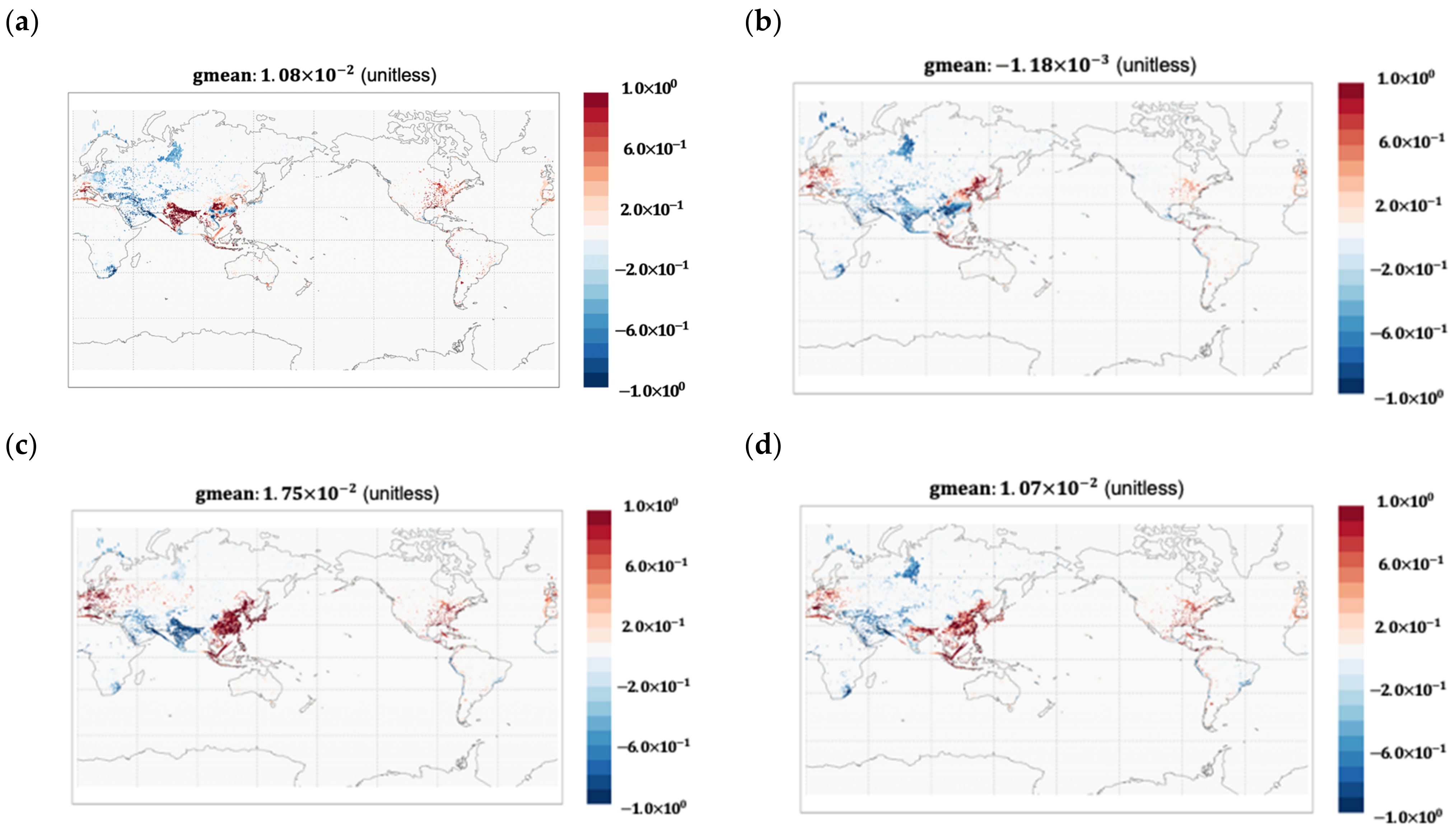
3.1. Global Impacts of Updating Anthropogenic Emissions

We compared the global distribution patterns of simulated AODs (BASE, SENS1, and SENS2) with the ensemble simulations of the International Cooperative of Aerosol Predictions (ICAP) and MISR, VIIRS, and MODIS satellite observations (i.e., the “reference” data). The BASE simulation has smaller global mean biases against the reference data than SENS1 and SENS2 (Figure 7). Figure 7 shows that the model biases in MAM are the largest against MODIS and the smallest against MISR. The negative biases are prevalent over the ocean and cover the Tibetan Plateau and Central Africa, while the positive biases appear in East Asia. There are strong positive biases in the East Asia region in BASE. These positive biases are reduced when updating to the CEDS 2019 emissions data in SENS1; however, the negative biases over the other land regions and the oceans are persistent, especially against MODIS and VIIRS. SO₂ bias scaling reduces the magnitudes of the global mean biases of SENS2 (Figure 6b).

Figure A1, Figure A2 and Figure A3 shows the global distributions of model biases against various references in DJF, from June to August (JJA), and SON. In DJF, the positive biases extend to Siberia, Eastern Europe, and the Northwestern Pacific, resulting in positive or reduced negative global mean biases (GMBs). The bias patterns of SENS1 and SENS2 against the reference data are very similar (Figure 7, Figure A1, Figure A2 and Figure A3). However, SENS2 has a smaller magnitude of biases in MAM and from June to August (JJA) than SENS1, while SENS2 has a larger magnitude of biases in the DJF and SON seasons. These bias changes are caused by the bias-scaled SO₂ emissions for SENS2 in India, Asia, and Western Europe (Figure 6b). Increasing the CEDS 2019 SO₂ emissions in these regions, especially for India, generally reduces the global mean underpredictions in DJF and SON. In contrast, reducing the CEDS 2019 SO₂ emissions increases the underpredictions in MAM and JJA (Figure 7, Figure A1, Figure A2 and Figure A3).

The GMBs of the modeled AODs in four seasons vary with references (Figure 8). For VIIRS and MODIS, the magnitudes of GMB of SENS1 and SENS2 are larger than those of BASE in all four seasons. For MISR, the former is smaller than the latter in DJF and SON. For ICAP, the magnitudes of GMB of SENS1 and SENS2 are larger than those of BASE in DJF, while the former is smaller than the latter in SON.

The negative global mean biases are the largest against MODIS in all four seasons (Figure 8). The negative biases against ICAP appear over the oceans, India, and the continent in the southern hemisphere in all four seasons, and Africa in MAM (Figure 7) and SON (Figure A2). The biases against MISR are the least negative among the reference data (Figure 7), mainly due to the reduced negative biases over the oceans (Figure 7, Figure A1, Figure A2 and Figure A3). They are even positive in DJF for all three modeled AODs (Figure 7), due to the positive Biases in Europe, Northern Africa, Asia, and the Northwest Pacific regions (Figure A3). The modeled AOD biases against VIIRS and MODIS have similar spatial features in terms of the global distributions in MAM, such as the large negative biases over the oceans and Himalayan mountains and the large positive biases in East Asia (Figure 7). The biases against VIIRS are increasingly negative over the Tibetan Plateau in the SON and DJF seasons (Figure A2 and Figure A3). The negative bias over the oceans is the largest against MODIS, resulting in the most negative GMBs among the reference data (Figure 8).

The biases against the satellite observations and the ICAP of ensemble simulation data turn out the wide ranges of biases between reference types and seasons. Global mean biases vary with reference types by a factor of 3~13 and season by 2~10. Overall, the magnitudes of the global mean biases are the largest in MODIS and the smallest in MISR. On the other hand, the negative biases are the largest in MAM and the smallest in DJF. Due to such large ranges of biases against those references, model biases need to be examined by the references using a different observation platform.

As an objective evaluation method against independent ground-truth measurements, all available global AERONET AOD (version 3 direct sun and inversion algorithm, i.e., Level 1.5) data were collected. The globally averaged Person’s correlation coefficient(r) and Index of Agreement (IOA) for SENS2 improved (i.e., increased) compared to SENS1 in the four seasons (Figure 9). The global mean biases of SENS1 and SENS2 were negative compared to the BASE case; however, the negative biases of SENS2 were reduced compared with those of SENS1, except in the MAM season. SO₂ bias scaling in SENS2 increased the global mean correlation and IOA by 0.74~5.52% and 0~4.86%, respectively, compared to AERONET in DJF, JJA, and SON. The greatest improvement appeared in DJF; however, the degradation of model correlation and IOA occurred in MAM. Global seasonal mean biases decreased in MAM, JJA, and SON by 13.0~26.9%. The biases decreased most in JJA; however, they increased by 16.7% in MAM (Figure 9e–g).

SO₂ bias scaling exacerbated the negative biases to increase the GMBs (Figure 7, Figure A1, Figure A2 and Figure A3); however, it reduced the magnitude of most of the regional mean biases (Figure 10c). To investigate the regional biases, we classified 13 global regions where the biases against the references were distinct (Figure 10a). The scatter plots of the modeled AODs and AERONET AODs are shown in Figure 11, and the corresponding numerics are shown in Figure 10b–d. The number of AERONET sites differs with regions, due to the availability of AERONET sites. The 1:1 line helps to indicate an underestimation or overestimation of the modeled AODs against the observed AODs (Figure 11). The underestimations appear in Southeast Asia, India, and South America, while overestimates appear in East CONUS and the North Tropical Atlantic. Good correlations appear in East Asia, West CONUS, Europe, and North Africa. Figure 10b–d shows that bias scaling improves all the numerical statistics in terms of the model’s performance against AERONET AODs in East Asia, West CONUS, and Southeast Asia. At the same time, it is worse in Saudi Arabia, South America, and the South Pacific relative to SENS1.

There is evidence of increases in r for SENS2 compared to SENS1 in most of the 13 regions analyzed, except Saudi Arabia and the Southern Pacific. The IOAs also increase in East Asia, Southeast Asia, Europe, Central and South Africa, and West CONUS. The regional mean biases are reduced in East Asia, Southeast Asia, North Tropical Atlantic, and West CONUS. Some numerical results will be discussed later. Overall, all the r, MB, and IOA values improve in East Asia, Southeast Asia, and West CONUS in SENS2 due to the bias scaling of SO₂; however, they become worse in Saudi Arabia and South Pacific in SENS2 compared to SENS1.

The annual average correlations increase for SENS2 across most regions by 0.0~18.7%; however, they decrease in the South Pacific by 2.28%. The annual IOAs increase in West CONUS, East Asia, Europe, and Africa by 0.22~3.39% for SENS2. However, the annual IOAs do not change in the North Tropical Atlantic, decreasing by 0.16~2.77% in other regions. The annual mean biases are reduced in West CONUS, North Tropical Atlantic, East Asia, and Southeast Asia by 38.3~4.85%, while the bias increases for SENS2 in the remaining global regions.

Overall, the bias-scaling methods improve in East Asia, Southeast Asia, and West CONUS, with annual mean correlations for SENS2 that improved by 4.3%, 1.5% and 0.4%, IOAs that improved by 3.30%, 3.4%, and 0.2%, and mean biases that improved by −38.3%, −4.9%, and −33.3%, respectively. In the ocean region, bias scaling leads to a decline in the annual mean correlation by 2.3% and a decrease in the IOA by 1.1% in the South Pacific, while the mean biases decrease by 12.5% in the North Tropical Atlantic. Furthermore, in other regions, bias scaling degrades the GEFS-Aerosols model’s performance in East CONUS, South America, India, Africa, and Saudi Arabia, with increasing mean biases and decreasing IOA values (except in Africa). Even though the correlation in India drastically increases, the negative MB also increases, and the IOA decreases (Figure 11f). To investigate the regional impacts of SO₂ bias scaling, we examined East Asia and India, where the impacts of updating SO₂ emissions data are noteworthy.

3.2. Regional Impacts in East Asia and India

In East Asia, box–whisker analyses of modeled vs. reference AODs show that AERONET AODs are smaller than VIIRS or MODIS, while they are larger than MERRA2 and MISR (Figure 12a). BASE overestimates against all the references, including MERRA2, and is larger than SENS1 and SENS2. SENS1 and SENS2 underestimate against MERRA2 and most of the observations, except MISR. The bias-scaling method increases the AOD in East Asia, resulting in SENS2 being larger than SENS1, and closer to AERONET. The seasonal scatter plots show that SENS2 has the highest correlation and IOA compared to AERONET among the three simulations, and it has reduced the negative mean biases compared to SENS1. SENS2 has the highest correlation and IOA in the JJA seasons and the least biases in MAM (Figure 12b–e). However, SENS2 has the largest improvement in correlation by 16.0%, IOA by 14.6% in DJF, and mean bias by 100.0%, which becomes 0 in MAM (Figure 12c).

In India, the three modeled AODs are underestimated against AERONET ground truth and all the additional reference data, while BASE is larger than both SENS1 and SENS2 (Figure 13). All the other reference data, except MODIS, are smaller than AERONET. The bias-scaling method increases the median AOD; however, both SENS1 and SENS2 have significantly smaller box–whisker values than AERONET. The annual scatter plot clearly shows the underpredicted AOD for all three simulations against AERONET (Figure 13b). In this case, the bias-scaling methods reduce the underpredictions in fall–winter (SON/DJF) but exacerbate the negative biases in the spring and summer (MAM/JJA) compared to SENS1 (Figure 13e). The correlations and IOAs are also improved in the bias-scaling SENS2 simulation for fall–winter. However, they are reduced compared to SENS1 during the spring and summer (Figure 13d).

We note that the bias-scaling factors in India increase the SO₂ emissions in DJF and SON (associated with improved model performance compared to AERONET) and decrease the emissions in MAM and JJA (associated with degraded model performance compared to AERONET). MERRA2 sulfate AODs were used for the SO₂ emissions bias scaling, but the MERRA2 total AODs were smaller than AERONET in India (Figure 13a). Thus, this result represents a limitation of our bias-scaling methods, which exhibit certain deficiencies when using assimilated MERRA2 data that do not agree with AERONET AOD observation, and likely highly uncertain compositional fractions of the total aerosol in certain regions, such as India. In other words, the exacerbated AOD biases for SENS2 in some seasons in India (e.g., spring–summer) imply that sulfate may not dominate. There are prolific natural emissions in India during the spring (MAM), such as biomass-burning aerosols transported from Southeast Asia. There is also mineral dust from Pakistan and the Arabian sea during the monsoon season in the summer (JJA). Therefore, it is likely that anthropogenic SO₂ emissions (and resulting sulfate aerosols) contribute less than the natural aerosols to the total AOD and thus limit the effectiveness of the bias-scaling approach used here.

4. Discussion

The SO₂ emission bias-scaling method that uses the relationship of the differences in SO₂ emissions relative to the differences in sulfate AODs between GEFS-Aerosols and MERRA2 can drastically improve GEFS-Aerosols SENS2 simulations, where anthropogenic SO₂ emissions are dominant sources of the total aerosol formation. In such regions, model performance is insensitive to seasonal aerosol emissions, but is sensitive to seasonal SO₂ emission scaling. In addition, the MERRA2 AOD is comparable to AERONET AODs. However, the bias-scaling method does not work well when the total AODs are sensitive to seasonal aerosol emissions, and natural emissions and transport dominate the total aerosol abundance. When the MERRA2 AODs have a more considerable bias against ground-truth observations (i.e., AERONET), SO₂ emissions bias scaling based on MERRA2 sulfate AODs departs from the ground-truth observations.

The advantage of this method is the ability to rapidly adjust emissions so that the model output is closer to the observation or assimilation data. One limitation is that we may miss essential mechanisms or processes that cause these differences, in addition to the emissions. For instance, SO₂ bias scaling is ineffective over the ocean, where GEFS-Aerosols intrinsically underestimates observations. Emission height also affects near-surface SO₂ and aerosol concentrations. Yang et al. [36] showed that the range in SO₂ surface concentrations caused by changing the emission height in one model was larger than the range in the diversity across models that simulated aerosol lifecycles [37]. The global distributions of SO₂ sectoral emissions provide hints on how to relate SO₂ emission types to emission height and receptor concentrations. In a future study, it would be useful to compare the model with the reference datasets for 2019 (or a common year when emissions data are available) to identify where the potential issues originate—either the emissions, model or reference data—and to extend the issue of updating to more recent years. On the other hand, a smaller magnitude of GMB does not always mean good model performance. The magnitude of GMB is small in regions with large positive and negative biases; however, it becomes large in locations where strong positive biases are reduced, such as in East Asia.

SO₂ emission bias scaling is assumed that MERRA2 assimilation data should be close to the observations. However, when we compared MERRA2 with the references and AERONET, we found that MEERA2 has biases. Therefore, this method becomes more reliable as the reference data adopted for bias scaling are accurate. In addition, the number of measurement sites (n) can affect the evaluations. For instance, there are fewer AERONET sites in Saudi Arabia (n = 87) and India (n = 43) than in Asia (n = 669), Europe (n = 1141), and CONUS (n = 541 for East or n = 791 for West). Bias-scaling results are more convincing in the latter regions than in the former. On the other hand, the co-existence of anthropogenic aerosols causes difficulty in the separation or speciation of aerosols through the current observed total AODs. It is necessary for a companion study on the emission scaling of anthropogenic absorbing aerosols, such as organic and black carbon, to be carried out. Therefore, using multi-platform and multi-species observation data will reduce such problems and support generalizing bias-scaling method.

5. Summary and Conclusions

Anthropogenic aerosol emissions reflect human activities and play a vital role in global AAC forecast models. For the GEFS-Aerosol AAC simulations in 2021, we updated the anthropogenic emission data (from CEDS 2014 to CEDS 2019) and used a simple SO₂ bias-scaling method to refine the updated SO₂ emissions further. We conducted a BASE simulation with CEDS 2014 emissions, a SENS1 simulation with CEDS 2019 emissions, and a SENS2 simulation with bias-scaled CEDS 2019 SO₂ emissions for sulfate AODs. Monthly bias-scaling factors were obtained by the regression analysis of the differences in the SO₂ emissions of CEDS 2019 and the sulfate AODs between GEFS-Aerosol simulations and MERRA2.

• Evaluations of the model AOD against ICAP, MERRA2 assimilation data, and a suite of satellite data, such as MISR, VIIRS, MODIS, and ground-truth AERONET, showed that the SENS1 model’s performance improved compared to BASE, particularly in East Asia, while SENS2 bias scaling led to a further improvement in model performance.
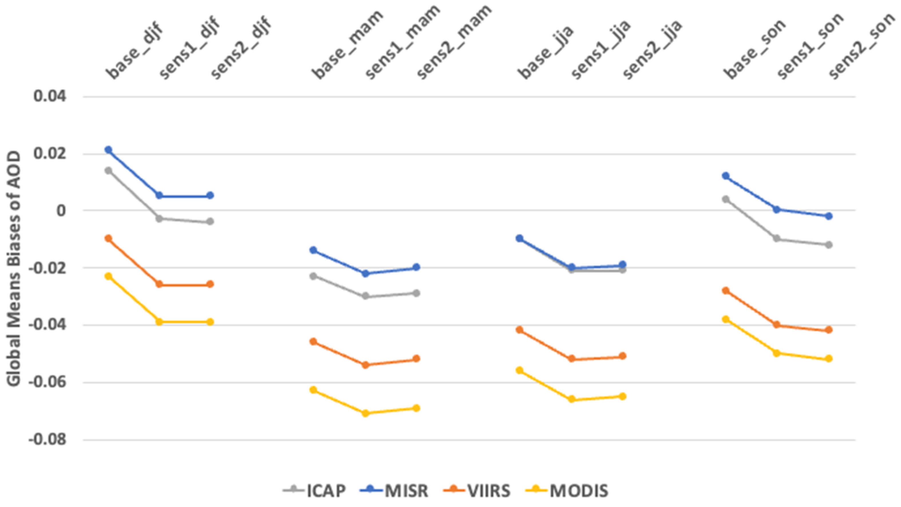
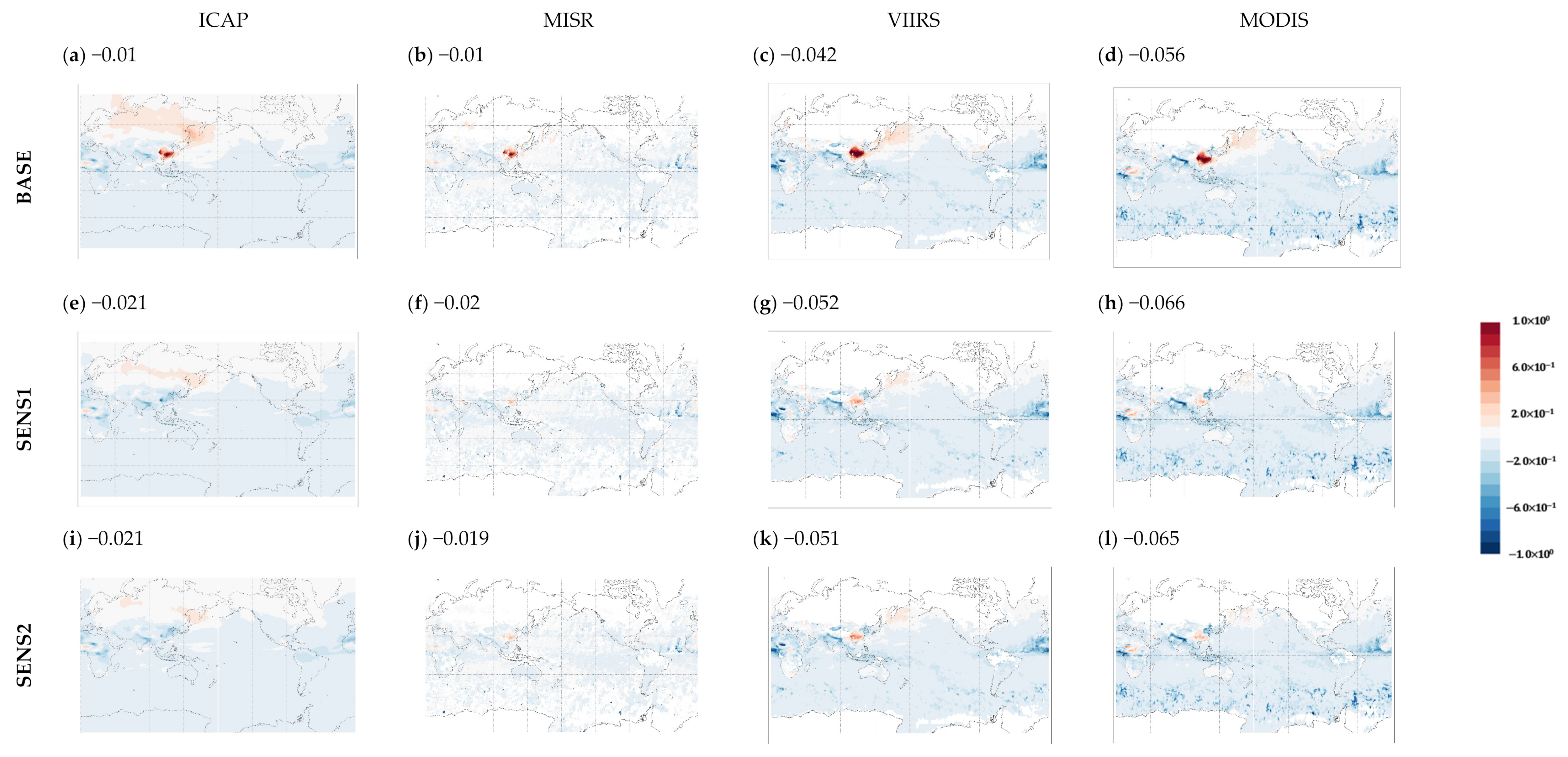
• The biases against the satellite observations and the ICAP of ensemble simulation data showed a wide range of biases between the references and seasons. The global mean biases varied with reference types by a factor of 3~13 and season by 2~10.
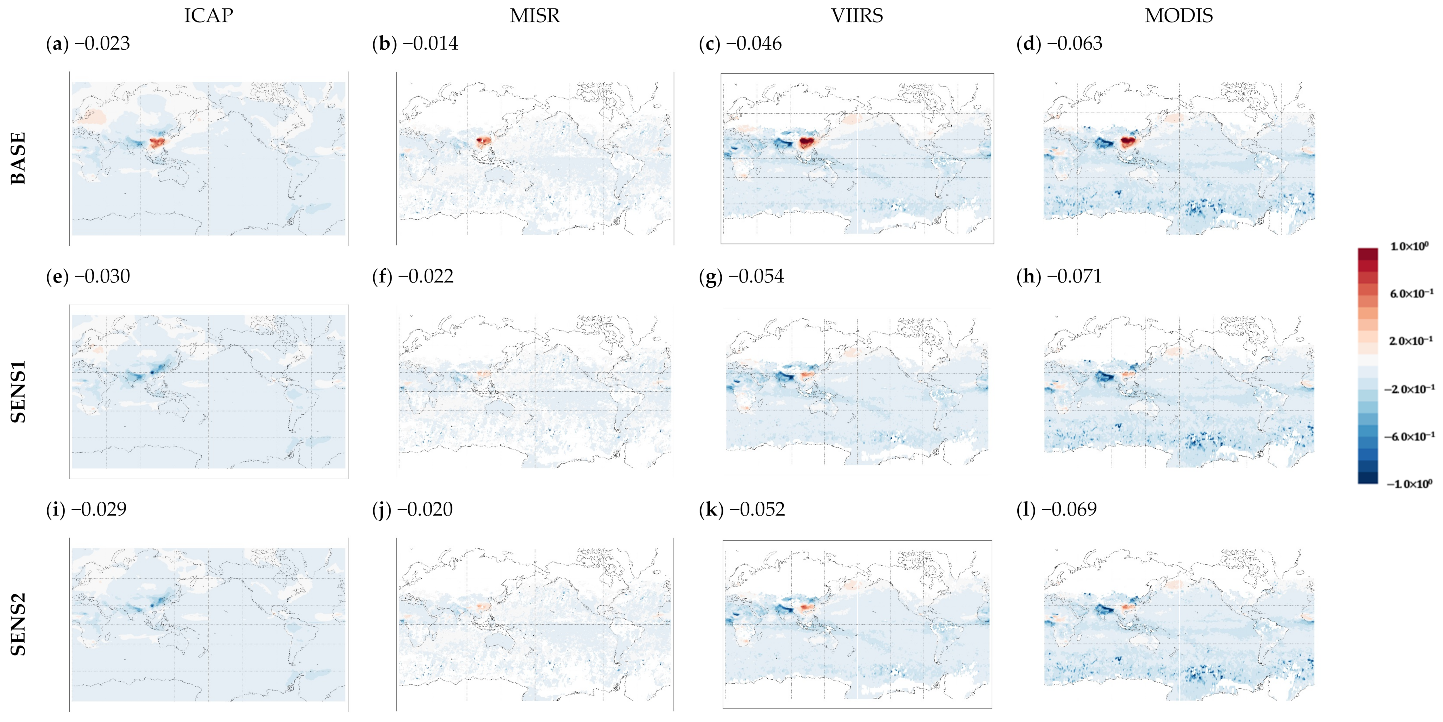
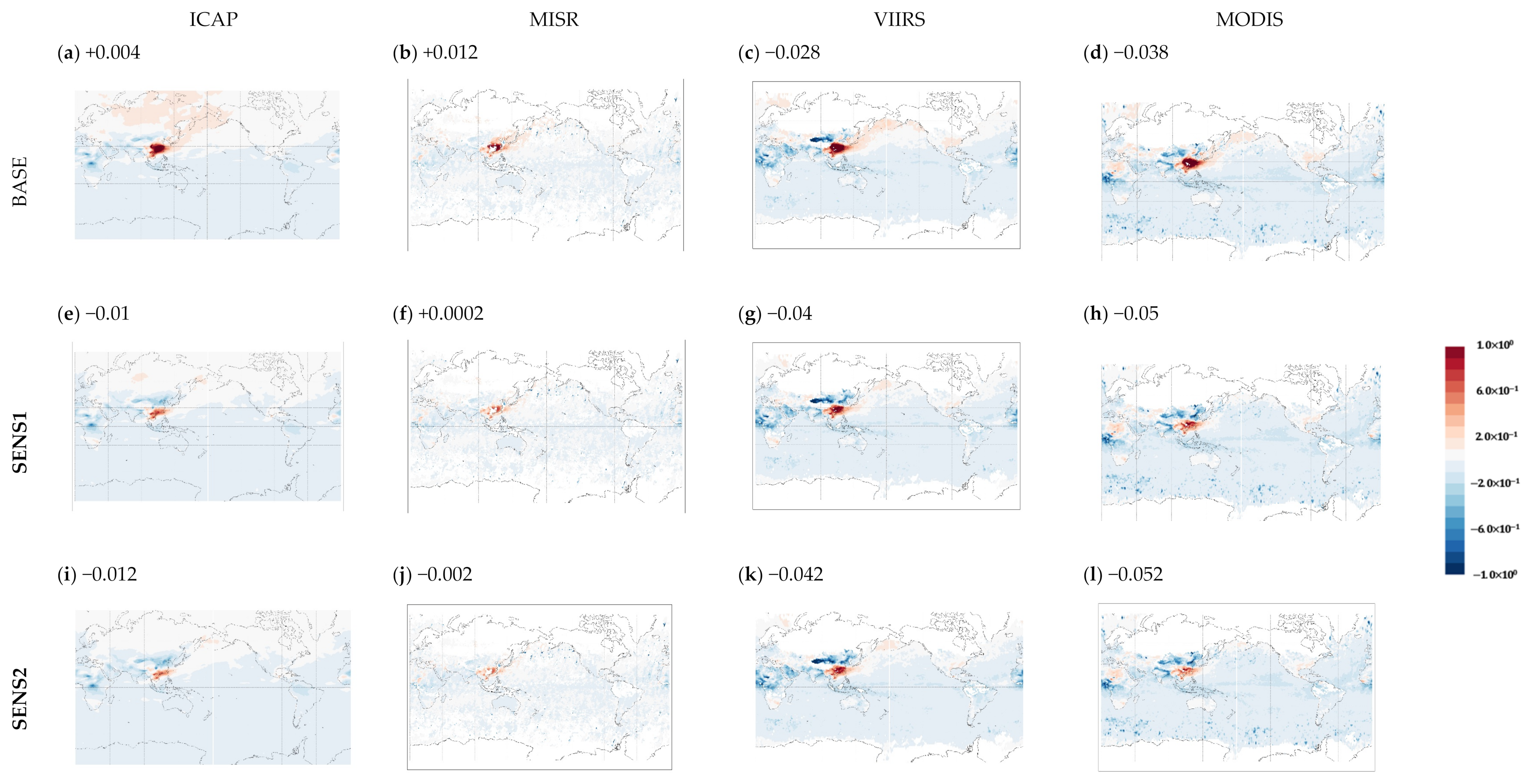
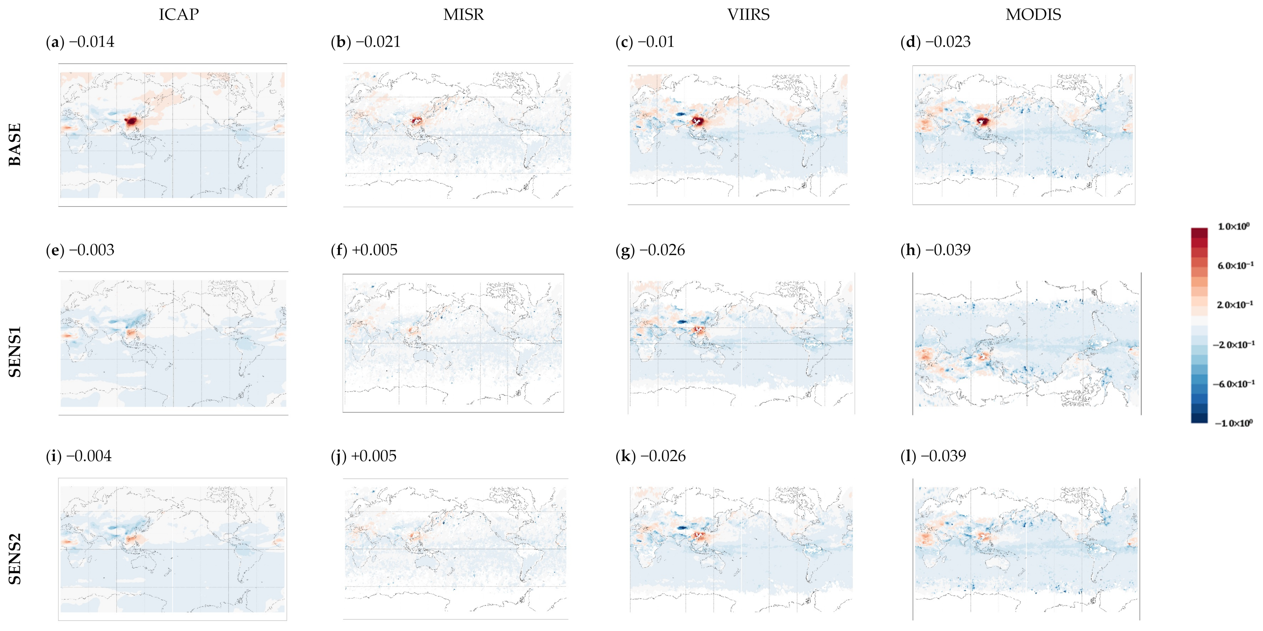
• Seasonally, the global AOD distributions showed that the differences in all the simulations against ICAP, MISR, VIIRS, and MODIS (i.e., the references) were the largest in MAM and the smallest in DJF. The biases against MISR were the least negative among the references, due to the relatively lower underpredictions against MISR over the oceans. The modeled AOD biases against both VIIRS and MODIS had very similar features in their global distributions; however, the modeled AOD had the most negative global mean biases against MODIS.
• The smaller magnitudes of GMB do not always mean better simulations, particularly when the upper and lower bounds of biases have different signs in different domains and are localized in specific regions, such as East Asia.
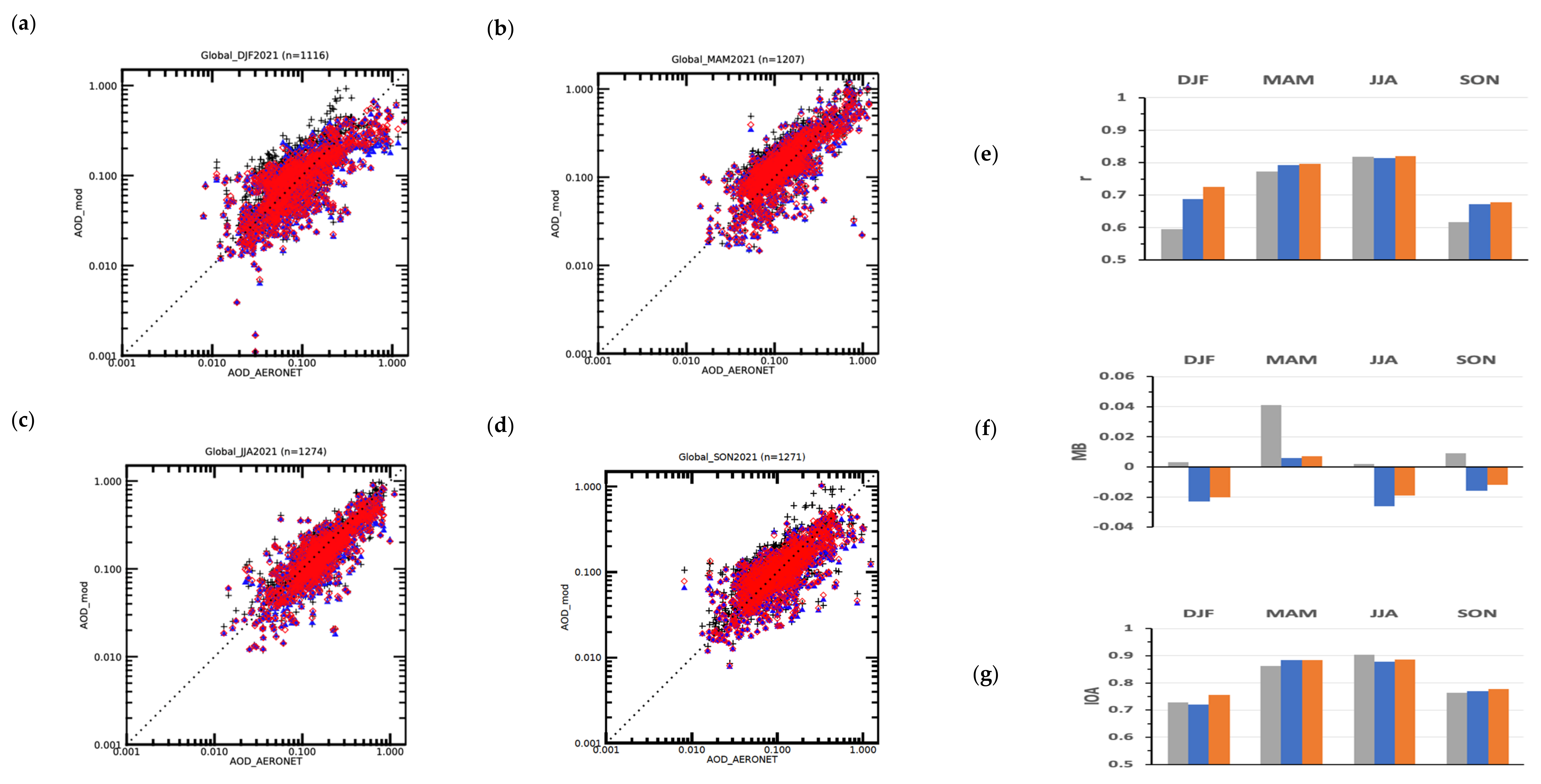
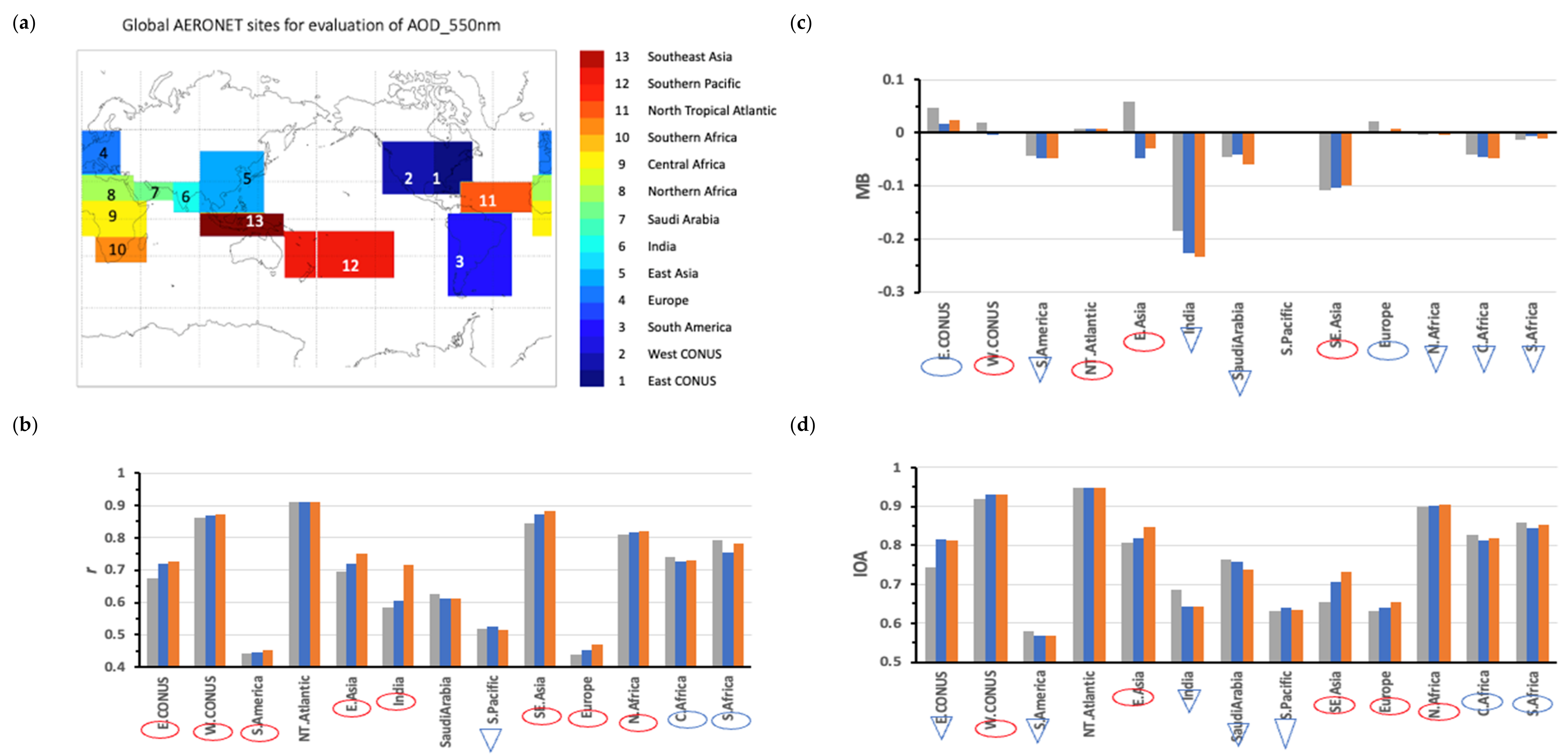
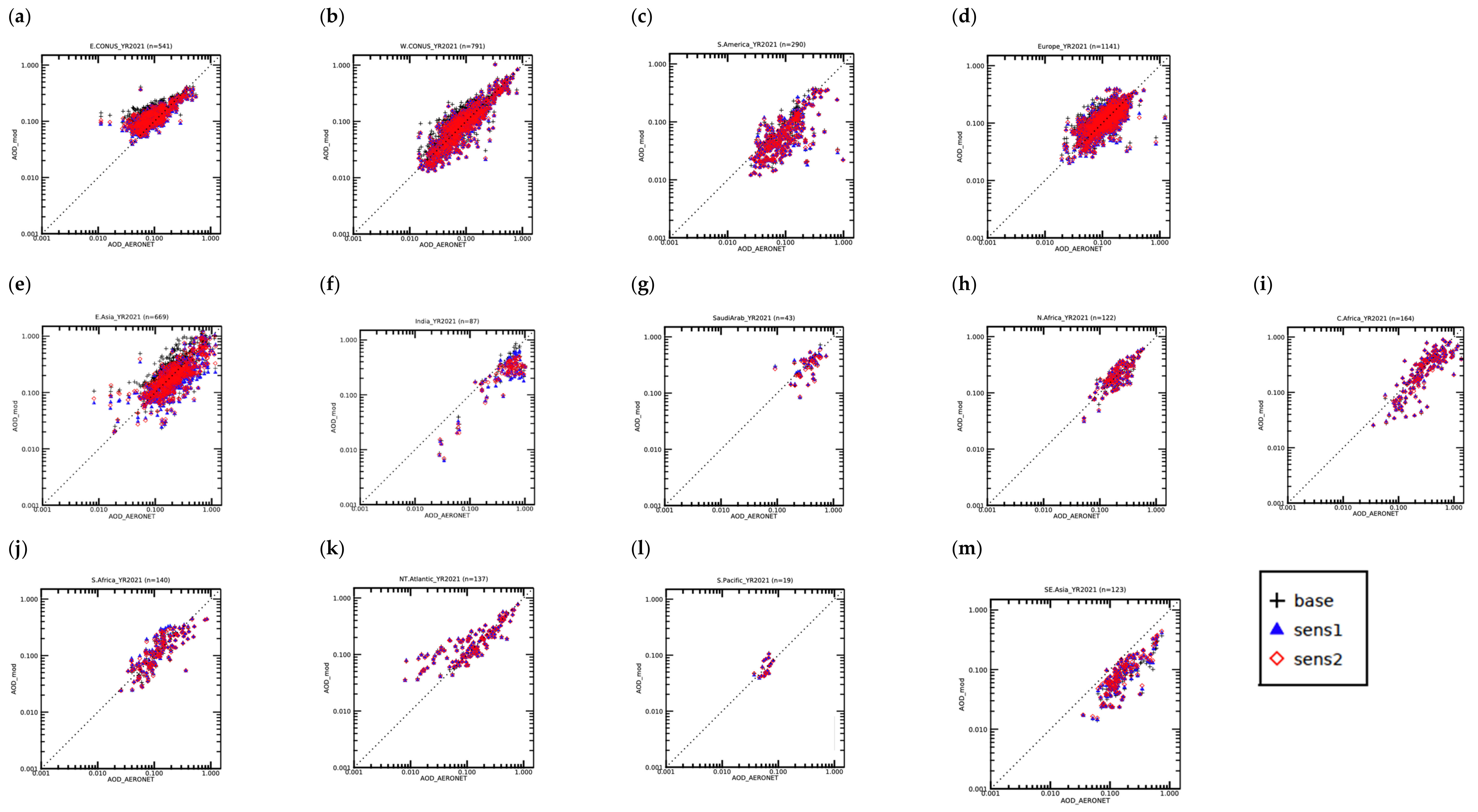
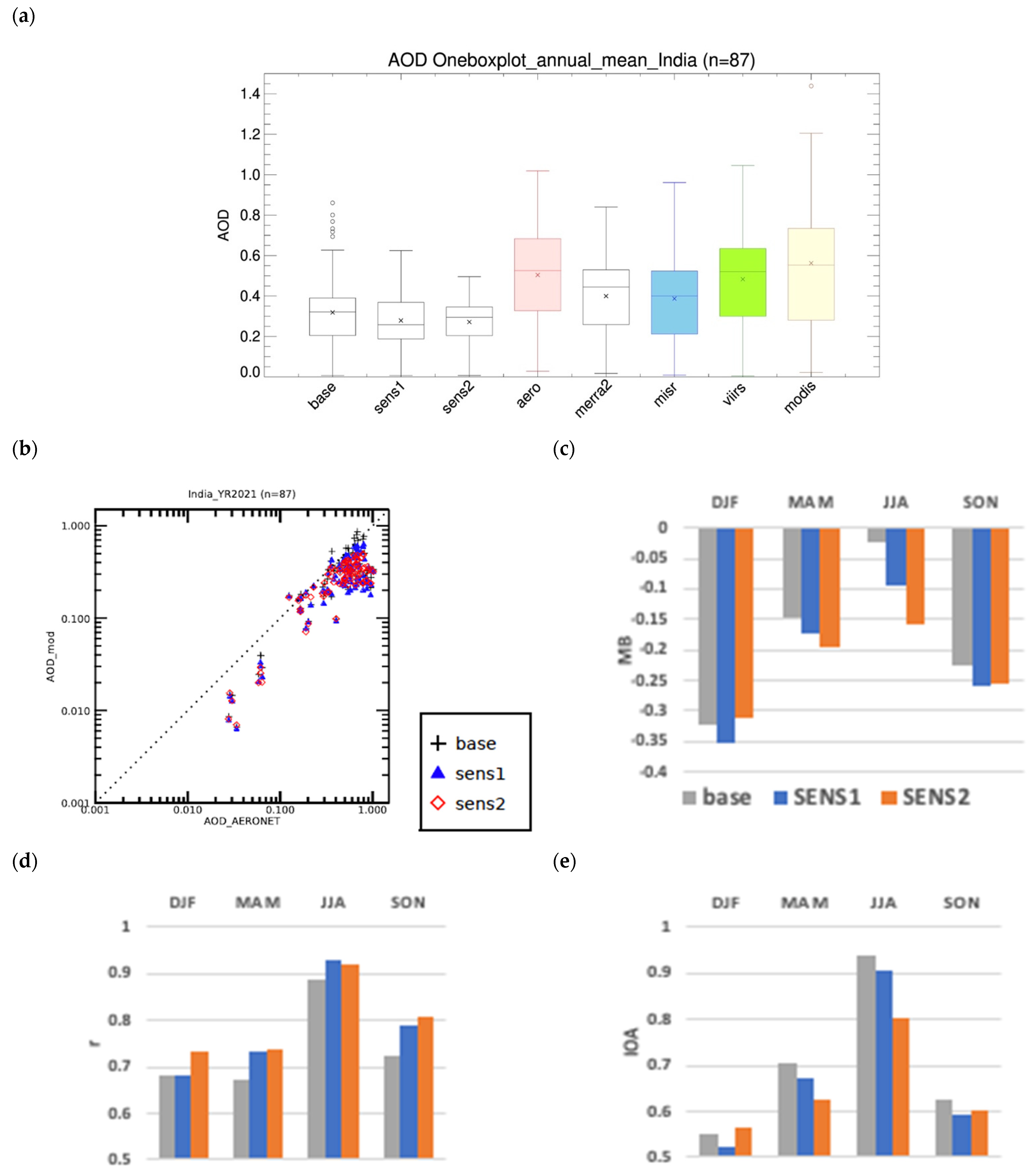
• AERONET AODs fell between MISR and MODIS AODs. Comparing the simulated AODs with AERONET data, the bias-scaling methods improved the global seasonal Pearson’s correlation (r), Index of Agreement (IOA), and mean bias (MB), except for the global mean biases in MAM, in which the negative regional biases were reduced more than the positive regional biases.
• Regionally, the SO₂ bias scaling showed the largest improvement in r, MB, and IOA in East Asia. On the other hand, the model performance in India improved for DJF and SON, but worsened in MAM and JJA. This seasonal contrast effect is due to the bias-scaled reductions in SO₂ emissions in India, along with the relatively more significant contributions from the other types of aerosols transported to this region.
• The simple bias-scaling methods work best in the regions where anthropogenic emissions are predominant, and the assimilated AOD speciation (e.g., MERRA2) represents the fractional contribution of aerosol composition well; however, the methodology for scale emissions works less well in regions that experience a large aerosol burden from natural phenomena, such as dust events, biomass burning, and sea salt.

Overall, a simple SO₂ bias-scaling method allows us to rapidly update anthropogenic emissions data using the available assimilated data to help improve the AAC model’s predictions of the global AOD. It is critical to fine-tune the specific regions globally to apply bias scaling (e.g., East Asia). In addition, bias scaling should also be applied to other anthropogenic emission sources of black and organic carbon aerosols (but only in regions outside of large dust or biomass-burning events) to improve AAC predictions further.

References

1. Cheewaphongphan, P.; Chatani, S.; Saigusa, N. Exploring Gaps between Bottom-Up and Top-Down Emission Estimates Based on Uncertainties in Multiple Emission Inventories: A Case Study on CH4 Emissions in China. Sustainability 2019, 11, 2054. [Google Scholar] [CrossRef] [Green Version]
2. Zheng, B.; Zhang, Q.; Geng, G.; Chen, C.; Shi, Q.; Cui, M.; Lei, Y.; He, K. Changes in China’s anthropogenic emissions and air quality during the COVID-19 pandemic in 2020. Earth Syst. Sci. Data 2021, 13, 2895–2907. [Google Scholar] [CrossRef]
3. Holoboff, J. Which is Better—Bottom-Up or Top-Down Emissions Estimates? 2021. Available online: https://processecology.com/articles/which-is-better-bottom-up-or-top-down-emissions-estimates#:~:text=A%20bottom%2Dup%20estimate%20is,in%20a%20bottom%2Dup%20approach (accessed on 1 September 2022).
4. Vaughn, T.L.; Bell, C.S.; Pickering, C.L.; Schwietzke, S.; Heath, C.A.; Petron, G.; Zimmerle, D.J.; Schnell, R.C.; Nummedal, D. Temporal variability largely explains top-down/bottom-up difference in methane emission estimates from a natural gas production region. Proc. Natl. Acad. Sci. USA 2018, 115, 11712–11717. [Google Scholar] [CrossRef] [PubMed] [Green Version]
5. Janssens-Maenhout, G.; Crippa, M.; Guizzardi, D.; Dentener, F.; Muntean, M.; Pouliot, G.; Keating, T.; Zhang, Q.; Kurokawa, J.; Wankmüller, R.; et al. HTAP_v2.2: A mosaic of regional and global emission grid maps for 2008 and 2010 to study hemispheric transport of air pollution. Atmos. Chem. Phys. 2015, 15, 11411–11432. Available online: https://edgar.jrc.ec.europa.eu/dataset_htap_v3/ (accessed on 1 September 2022). [CrossRef] [Green Version]
6. Crippa, M.; Guizzardi, D.; Muntean, M.; Schaaf, E.; Dentener, F.; van Aardenne, J.A.; Monni, S.; Doering, U.; Olivier, J.G.J.; Pagliari, V.; et al. Gridded emissions of air pollutants for the period 1970–2012 within EDGAR v4.3.2. Earth Syst. Sci. Data 2018, 10, 1987–2013. [Google Scholar] [CrossRef] [Green Version]
7. Klimont, Z.; Kupiainen, K.; Heyes, C.; Purohit, P.; Cofala, J.; Rafaj, P.; Borken-Kleefeld, J.; Schöpp, W. Global anthropogenic emissions of particulate matter including black carbon. Atmos. Chem. Phys. 2017, 17, 8681–8723. [Google Scholar] [CrossRef] [Green Version]
8. Hoesly, R.M.; Smith, S.J.; Feng, L.; Klimont, Z.; Janssens-Maenhout, G.; Pitkanen, T.; Seibert, J.J.; Vu, L.; Andres, R.J.; Bolt, R.M.; et al. 2018 Historical (1750–2014) anthropogenic emissions of reactive gases and aerosols from the Community Emissions Data System (CEDS). Geosci. Model Dev. 2018, 11, 369–408. [Google Scholar] [CrossRef] [Green Version]
9. McDuffie, E.E.; Smith, S.J.; O’Rourke, P.; Tibrewal, K.; Venkataraman, C.; Marais, E.A.; Zheng, B.; Crippa, M.; Brauer, M.; Martin, R.V. A global anthropogenic emission inventory of atmospheric pollutants from sector- and fuel-specific sources (1970–2017): An application of the Community Emissions Data System (CEDS). Earth Syst. Sci. Data 2020, 12, 3413–3442. Available online: https://github.com/JGCRI/CEDS/ (accessed on 1 September 2022). [CrossRef]
10. CEDS Version 2. Available online: https://dtn2.pnl.gov/data/gcam/CEDS_emissions/CEDS_gridded_data_2021-04-21/ (accessed on 1 September 2022).
11. Sicard, P.; De Marco, A.; Agathokleous, E.; Feng, Z.; Xu, X.; Paoletti, E.; Rodriguez, J.; Calatayud, V. Amplified ozone pollution in cities during the COVID-19 lockdown. Sci. Total Environ. 2020, 735, 139542. [Google Scholar] [CrossRef]
12. Goldberg, D.L.; Anenberg, S.C.; Griffin, D.; McLinden, C.A.; Lu, Z.; Streets, D.G. Disentangling the impact of the COVID-19 lockdowns on urban NO2 from natural variability. Geophys. Res. Lett. 2020, 47, e2020GL089269. [Google Scholar] [CrossRef]
13. Berman, J.D.; Ebisu, K. Changes in U.S. air pollution during the COVID-19 pandemic. Sci. Total Environ. 2020, 739, 139864. [Google Scholar] [CrossRef]
14. Li, L.; Li, Q.; Huang, L.; Wang, Q.; Zhu, A.; Xu, J.; Liu, Z.; Li, H.; Shi, L.; Li, R.; et al. Air quality changes during the COVID-19 lockdown over the Yangtze River Delta Region: An insight into the impact of human activity pattern changes on air pollution variation. Sci. Total Environ. 2020, 732, 139282. [Google Scholar] [CrossRef]
15. Liu, F.; Page, A.; Strode, S.A.; Yoshida, Y.; Choi, S.; Zheng, B.; Lamsal, L.N.; Li, C.; Krotkov, N.A.; Eskes, H.; et al. Abrupt decline in tropospheric nitrogen dioxide over China after the outbreak of COVID-19. Sci. Adv. 2020, 6, eabc2992. [Google Scholar] [CrossRef]
16. Shi, Z.; Song, C.; Liu, B.; Lu, G.; Xu, J.; Van Vu, T.; Elliott, R.J.R.; Li, W.; Bloss, W.J.; Harrison, R.M. Abrupt but smaller than expected changes in surface air quality attributable to COVID-19 lockdowns. Sci. Adv. 2021, 7, eabd6696. [Google Scholar] [CrossRef]
17. Le Quéré, C.; Jackson, R.B.; Jones, M.W.; Smith, A.J.P.; Abernethy, S.; Andrew, R.M.; De-Gol, A.J.; Willis, D.R.; Shan, Y.; Canadell, J.G.; et al. Temporary reduction in daily global CO2 emissions during the COVID-19 forced confinement. Nat. Clim. Change 2020, 10, 647–653. [Google Scholar] [CrossRef]
18. Campbell, P.C.; Tong, D.; Tang, Y.; Baker, B.; Lee, P.; Saylor, R.; Stein, A.; Ma, S.; Lamsal, L.; Qu, Z. Impacts of the COVID-19 economic slowdown on ozone pollution in the U.S. Atmos. Environ. 2021, 264, 118713. [Google Scholar] [CrossRef]
19. Wang, X.; Zhang, R. How Did Air Pollution Change during the COVID-19 Outbreak in China? Bull. Am. Meteorol. Soc. 2020, 101, E1645–E1652. Available online: https://journals.ametsoc.org/view/journals/bams/101/10/bamsD2001 (accessed on 1 February 2022). [CrossRef]
20. Miyazaki, K.; Bowman, K.; Sekiya, T.; Jiang, Z.; Chen, X.; Eskes, H.; Ru, M.; Zhang, Y.; Shindell, D. Air quality response in China linked to the 2019 novel coronavirus (COVID-19) lockdown. Geophys. Res. Lett. 2020, 47, e2020GL089252. [Google Scholar] [CrossRef]
21. Xu, J.; Ge, X.; Zhang, X.; Zhao, W.; Zhang, R.; Zhang, Y. COVID-19 impact on the concentration and composition of submicron particulate matter in a typical city of Northwest China. Geophys. Res. Lett. 2020, 47, e2020GL089035. [Google Scholar] [CrossRef]
22. Le, T.; Wang, Y.; Liu, L.; Yang, J.; Yung, Y.L.; Li, G.; Seinfeld, J.H. Unexpected air pollution with marked emission reductions during the COVID-19 outbreak in China. Science 2020, 369, 702–706. [Google Scholar] [CrossRef]
23. Tang, Y.; Pagowski, M.; Chai, T.; Pan, L.; Lee, P.; Baker, B.; Kumar, R.; Delle Monache, L.; Tong, D.; Kim, H.-C. A case study of aerosol data assimilation with the Community Multi-scale Air Quality Model over the contiguous United States using 3D-Var and optimal interpolation methods. Geosci. Model Dev. 2017, 10, 4743–4758. [Google Scholar] [CrossRef] [Green Version]
24. Tang, Y.; Tong, D.Q.; Yang, K.; Lee, P.; Baker, B.; Crawford, A.; Luke, W.; Stein, A.; Campbell, P.C.; Ring, A.; et al. Air quality impacts of the 2018 Mt. Kilauea Volcano eruption in Hawaii: A regional chemical transport model study with satellite-constrained emissions. Atmos. Environ. 2020, 237, 117648. [Google Scholar] [CrossRef]
25. Zhang, L.; Montuoro, R.; McKeen, S.A.; Baker, B.; Bhattacharjee, P.S.; Grell, G.A.; Henderson, J.; Pan, L.; Frost, G.J.; McQueen, J.; et al. Development and evaluation of the Aerosol Forecast Member in the National Center for Environment Prediction (NCEP)’s Global Ensemble Forecast System (GEFS-Aerosols v1). Geosci. Model Dev. 2022, 15, 5337–5369. [Google Scholar] [CrossRef]
26. Chin, M.; Ginoux, P.; Kinne, S.; Holben, B.N.; Duncan, B.N.; Martin, R.V.; Logan, J.A.; Higurashi, A.; Nakajima, T. Tropospheric aerosol optical thickness from the GOCART model and comparisons with satellite and sunphotometer measurements. J. Atmos. Sci. 2002, 59, 461–483. [Google Scholar] [CrossRef]
27. Chin, M.; Rood, R.B.; Lin, S.-J.; Muller, J.F.; Thomspon, A.M. Atmospheric sulfur cycle in the global model GOCART: Model description and global properties. J. Geophys. Res. 2000, 105, 24671–24687. [Google Scholar] [CrossRef]
28. Randles, C.A.; da Silva, A.M.; Buchard, V.; Colarco, P.R.; Darmenov, A.; Govindaraju, R.; Smirnov, A.; Holben, B.; Ferrare, R.; Hair, J.; et al. The MERRA-2 Aerosol Reanalysis, 1980 Onward. Part I: System Description and Data Assimilation Evaluation. J. Clim. 2017, 30, 6823–6850. Available online: https://journals.ametsoc.org/view/journals/clim/30/17/jcli-d-16-0609.1.xml (accessed on 15 January 2022). [CrossRef]
29. Lamarque, J.-F.; Bond, T.C.; Eyring, V.; Granier, C.; Heil, A.; Klimont, Z.; Lee, D.; Liousse, C.; Mieville, A.; Owen, B.; et al. Historical (1850–2000) gridded anthropogenic and biomass burning emissions of reactive gases and aerosols: Methodology and application. Atmos. Chem. Phys. 2010, 10, 7017–7039. [Google Scholar] [CrossRef] [Green Version]
30. Black, T.L.; Abeles, J.A.; Blake, B.T.; Jovic, D.; Rogers, E.; Zhang, X.; Aligo, E.A.; Dawson, L.C.; Lin, Y.; Strobach, E.; et al. A limited area modeling capability for the Finite-Volume Cubed- Sphere (FV3) dynamical core and comparison with a global two-way nest. J. Adv. Model. Earth Sys. 2021, 13, e2021MS002483. [Google Scholar] [CrossRef]
31. Zhou, X.; Zhu, Y.; Hou, D.; Fu, B.; Li, W.; Guan, H.; Sinsky, E.; Kolczynski, W.; Xue, X.; Luo, Y.; et al. The Development of the NCEP Global Ensemble Forecast System Version 12. Weather Forecast. 2022, 37, 1069–1084. Available online: https://journals.ametsoc.org/view/journals/wefo/37/6/WAF-D-21-0112.1.xml (accessed on 1 August 2022).
32. Yang, F. Implementation, and evaluation of the NOAA Next Generation Global Prediction System with FV3 Dynamic Core and Advanced Physics. In Proceedings of the 98th American Meteorological Society Conference, Austin, TX, USA, 7–11 June 2018; Available online: https://ams.confex.com/ams/98Annual/webprogram/Paper329963.html (accessed on 15 October 2022).
33. Campbell, P.C.; Baker, B.; Tong, D.; Saylor, R. Initial Development of a NOAA Emissions and eXchange Unified System (NEXUS). In Proceedings of the 100th American Meteorological Society Conference, Boston, MA, USA, 12–16 January 2020. [Google Scholar] [CrossRef]
34. Lin, H.; Jacob, D.J.; Lundgren, E.W.; Sulprizio, M.P.; Keller, C.A.; Fritz, T.M.; Eastham, S.D.; Emmons, L.K.; Campbell, P.C.; Baker, B.; et al. Harmonized Emissions Component (HEMCO) 3.0 as a versatile emissions component for atmospheric models: Application in the GEOS-Chem, NASA GEOS, WRF-GC, CESM2, NOAA GEFS-Aerosol, and NOAA UFS models. Geosci. Model Dev. 2021, 14, 5487–5506. [Google Scholar] [CrossRef]
35. Keller, C.A.; Long, M.S.; Yantosca, R.M.; Da Silva, A.M.; Pawson, S.; Jacob, D.J. HEMCO v1.0: A versatile, ESMF-compliant component for calculating emissions in atmospheric models. Geosci. Model Dev. 2014, 7, 1409–1417. Available online: www.geosci-model-dev.net/7/1409/2014/ (accessed on 15 February 2021). [CrossRef] [Green Version]
36. Yang, Y.; Smith, S.J.; Wang, H.; Lou, S.; Rasch, P.J. Impact of anthropogenic emission injection height uncertainty on global sulfur dioxide and aerosol distribution. J. Geophys. Res. Atmos. 2019, 124, 4812–4826. [Google Scholar] [CrossRef]
37. Textor, C.; Schulz, M.; Guibert, S.; Kinne, S.; Balkanski, Y.; Bauer, S.; Berntsen, T.; Berglen, T.; Boucher, O.; Chin, M.; et al. Analysis and quantification of the diversities of aerosol life cycles within AeroCom. Atmos. Chem. Phys. 2006, 6, 1777–1813. [Google Scholar] [CrossRef] [Green Version]
Figure 1. Global distributions of annual average emissions (Gg/m2/yr) of BC, OC and SO2 in CEDS 2014 (ac) and the differences between CEDS 2014 and CEDS 2019 (df) (the global annual total emissions (Tg/yr) are shown above the figures).
Atmosphere 14 00234 g001
Figure 2. The monthly global means of the differences in total and sectoral emissions (Gg/mon), such as agriculture (agr, in red), energy (ene, in gray), industry (ind, in yellow), residential_commercial_others (RCO, in blue), international shipping (shp, in green), solvent-production applications (slv, in light blue), road transportation (road, in peach), and waste (wst, in light grey) in CEDS 2014 from CEDS 2019 of (a) BC, (b) OC, and (c) SO2.
Atmosphere 14 00234 g002
Figure 3. The global distributions of annual SO2 sectoral emissions (Gg/m2/yr) in CEDS 2014 (sectoral emission names (af) and the global annual sectoral emissions (Tg/yr) are shown above the figures).
Atmosphere 14 00234 g003
Figure 4. (a) The regression of SO2 emissions (CEDS 2019) and SENS1 model sulfate AOD in October 2021. (b) Monthly values of the regressions in 2021. A high-to-low resolution, regional-scale filter (12° × 6°) was applied to both the model and emissions data for the regression. This amounts to a total of 900 grid points.
Atmosphere 14 00234 g004
Figure 5. The differences in GEFS sulfate AOD from (a) MERRA2 sulfate AOD and (b) the fractional differences in SO2 emissions, x-1, in October 2021. A comparison of global SO2 emissions between (c) CEDS 2019 and (d) after scaling application.
Atmosphere 14 00234 g005
Figure 6. Global distribution of the fractional differences in SO2 emissions, x -1, in (a) DJF, (b) MAM, (c) JJA, and (d) SON of 2021.
Atmosphere 14 00234 g006
Figure 7. Global distribution of the differences in GEFS AOD (BASE (ad), SENS1 (eh) and SENS2 (il)) from ensemble simulation of ICAP (a,e,i), and satellite observations of MISR (b,f,j), VIIRS (c,g,k), and MODIS (d,h,l) in MAM 2021 (the numbers above figures indicate the global mean (unitless)).
Atmosphere 14 00234 g007
Figure 8. Comparisons of global seasonal means of the differences in GEFS AOD (BASE1, SENS1 and SENS2) from ensemble simulation of ICAP and satellite observations of MISR, VIIRS, and MODIS.
Atmosphere 14 00234 g008
Figure 9. The scatter plots of global seasonal means of the GEFS AODs against AERONET AOD on global scales in (a) DJF, (b) MAM, (c) JJA and (d) SON of 2021 (n indicates the number of data points). (Black, blue, and red symbols indicate BASE, SENS1, and SENS2, respectively. The 1:1 dotted line is inset). Bar graphs in the right column are the statistics such as (e) correlation, (f) mean bias, and (g) Index of Agreement. (Gray, blue, and orange bars indicate BASE, SENS1, and SENS2, respectively).
Atmosphere 14 00234 g009
Figure 10. (a) Thirteen regions for the evaluation of SO2 emissions. (b) The correlation, (c) MB, and (d) IOA. Gray, blue, and orange bars indicate BASE, SENS1, and SENS2, respectively. Red circles over the region names indicate that SENS2 improved relative to SENS1. Inverted triangles indicate SENS2 deteriorated relative to SENS1. Additionally, blue circles indicate that SENS2 improved relative to SENS1; however, SENS2 deteriorated relative to BASE.
Atmosphere 14 00234 g010
Figure 11. The scatter plots of the annual mean of GEFS AODs against AERONET AOD in 13 regions, including (a) East CONUS, (b) West CONUI, (c) South America, (d) Europe, (e) East Asia, (f) India, (g) Saudi Arabia, (h) Northern Africa, (i) Central Africa, (j) Southern Africa, (k) North Tropical Atlantic, (l) South Pacific, and (m) Southeast Asia, in 2021. The 1:1 dotted line is inset.
Atmosphere 14 00234 g011
Figure 12. (a) The box and whisker plot of the annual AOD mean biases of BASE, SENS1, and SENS2 (first, second, and third column in white, respectively); AERONET (in pink); MERRA2 (5th column in white); MISR (in light blue); VIIRS (in green); and MODIS (in yellow) in East Asia. (b) The scatter plot of annual simulated AODs against AERONET AODs (the 1:1 dotted line is inset). (c) Seasonal mean biases, (d) seasonal correlations, and (e) seasonal IOAs.
Atmosphere 14 00234 g012
Figure 13. (a) The box and whisker plot of the annual AOD mean biases of BASE, SENS1, and SENS2 (first, second, and third column in white, respectively); AERONET (in pink), MERRA2 (5th column in white); MISR (in light blue), VIIRS (in green); and MODIS (in yellow) in India. (b) The scatter plot of the annual simulated AODs against AERONET AODs (the 1:1 dotted line is inset). (c) Seasonal mean biases, (d) seasonal correlations, and (e) seasonal IOAs.
Atmosphere 14 00234 g013