
Wildfires Impact Assessment on PM Levels Using Generalized Additive Mixed Models
by
 , ,
, ,
Gianluca Leone
*,
Giorgio Cattani
,
Mariacarmela Cusano
,
Alessandra Gaeta
,
Guido Pellis
,
Marina Vitullo
and
Raffaele Morelli
Department for Environmental Evaluation, Control and Sustainability, Italian National Institute for Environmental Protection and Research (ISPRA), 00144 Rome, Italy
*
Author to whom correspondence should be addressed.
Atmosphere 2023, 14(2), 231; https://doi.org/10.3390/atmos14020231
Submission received: 15 December 2022
/
Revised: 19 January 2023
/
Accepted: 20 January 2023
/
Published: 24 January 2023
(This article belongs to the Special Issue Air Quality, Health and Environmental Impact Assessment)
Abstract
:Wildfires are relevant sources of PM emissions and can have an important impact on air pollution and human health. In this study, we examine the impact of wildfire PM emissions on the Piemonte (Italy) air quality regional monitoring network using a Generalized Additive Mixed Model. The model is implemented with daily PM10 and PM2.5 concentrations sampled for 8 consecutive years at each monitoring site as the response variable. Meteorological data retrieved from the ERA5 dataset and the observed burned area data stored in the Carabinieri Forest Service national database are used in the model as explanatory variables. Spline functions for predictive variables and smooths for multiple meteorological variables’ interactions improved the model performance and reduced uncertainty levels. The model estimates are in good agreement with the observed PM data: adjusted R2 range was 0.63–0.80. GAMMs showed rather satisfactory results in order to capture the wildfires contribution: some severe PM pollution episodes in the study area due to wildfire air emissions caused peak daily levels up to 87.3 µg/m3 at the Vercelli PM10 site (IT1533A) and up to 67.7 µg/m3 at the Settimo Torinese PM2.5 site (IT1130A).
1. Introduction
According to the first part of the Sixth Assessment Report, Climate Change 2021: The Physical Science Basis [1], frequency, intensity and severity of wildfires will increase in many regions of the world due to climatic trends.
Indeed, global increases in average temperature; a rise in heatwave frequency, intensity, and/or extent; and drought periods lasting longer and extending over greater areas of time and space have all been related to the harshness of wildfires [2,3,4,5,6,7,8,9,10].
The Advance Report on Forest Fires in Europe, Middle East and North Africa 2021 [11] reported that in 2021, Turkey was the country with the most burnt area, followed by Italy, which was the country with the greatest number of fires.
Emissions from wildfires have a significant influence on atmospheric composition due to the large amounts of compounds emitted into the atmosphere during combustion, including carbon dioxide (CO2), carbon monoxide (CO), methane (CH4), nitrogen oxides (NOx), ammonia (NH3), particulate matter PM10 and PM2.5, non-methane hydrocarbon (NMHC), polycyclic aromatic hydrocarbons (PAHs), and other chemical species as well as volatile organic compounds (VOCs) [12,13,14,15,16,17,18,19,20]. Moreover, many wildland-fire-related compounds act as secondary organic aerosol (SOA) precursors, thereby contributing to its formation [21,22,23].
Wildland fire emissions can impact air quality locally, regionally [24,25,26], and over distances of several thousand kilometers [27,28,29].
Epidemiological studies aimed to assess the relationships between particle exposure (mainly PM10 and PM2.5) and health outcomes have been extensively carried out over the last two decades. PM exposure has been widely recognized to have an effect on cardiopulmonary diseases, lung cancer, and premature mortality [30,31,32,33,34,35,36,37,38,39].
Several studies were aimed at improving the wildfires air quality impact assessment as well as deepening our understanding of the relationship between wildfire emissions and human health effects [40,41,42]. Notably, a study on short-term effects of particulate matter PM10 on mortality during forest fires in Southern Europe [43] found that smoke was associated with increased cardiovascular mortality in urban residents, and PM10 on smoky days had a larger effect on cardiovascular and respiratory mortality than on other days.
In [44], evidence of an association of the exposure to long-range transported PM2.5 from vegetation fires over hundreds to thousands of kilometers, with the increase in cardiovascular mortality and, to a lesser extent, with the hospital admissions due to respiratory causes was provided.
Furthermore, fine particulate emissions from wildfires were associated with increased mortality rates on fire days with poor air quality [45,46], and with increased risks for specific groups of people, including the elderly [47], those with pre-existing respiratory conditions, and children [48,49].
The fires’ related atmospheric emissions have been found to also affect the ecosystems, particularly plant productivity downwind of fires through enhanced ozone [50] and aerosol concentrations [51].
Each year, 350 million hectares of vegetation are reported to be affected by fires around the world, half of them in sub-Saharan Africa [52].
Methods commonly used to quantify wildfire effects on the spatio-temporal variability of air pollutant concentrations, and therefore on human health and ecosystems, include: air pollution monitoring networks [45,53,54], land use regression modeling (LUR) [55,56,57,58,59,60], remote-sensing- or aerosol optical depth (AOD)-based models [61,62,63,64], estimates from satellite observations [61,65,66,67,68], low-cost sensor measurements [69,70], and chemical transport models (CTM) [66,71,72,73,74]. As each model has strengths and weaknesses, no single model should be considered as the most accurate to quantify human exposure to wildfire smoke [75]. Many regional fire studies with CTM have been undertaken to assess the impact of fire emissions on air pollution in populated areas of the world, such as in Europe [66,71,76]. In [77], the MM5/CHIMERE air quality modelling system predicted that Portugal’s future forest fire emissions will increase PM10 concentrations, especially where the burned area projections were higher, in detail + 20 μg/m3 along the Northern coastal region and + 32 μg/m3 over the center of the country.
Based on the available studies, the fires’ size appears as a key variable: small fires do not seem to affect mortality rate significantly, whereas medium and large fires (with burned areas > 1000 ha) showed a significant impact on human health, which increased with the extent of the fire [78,79].
At the local level, air quality can show strong spatio-temporal variation during wildfires depending on concurrent meteorology and synoptic circulation [80,81,82,83,84]. To study the relationship between fires and air pollutant levels at a seasonal timescale, distinguishing the contribution of local meteorological factors to relative concentrations, empirical models have also been used. In [85], using a multiple linear regression analysis, the seasonal variability of PM10 and PM2.5 due to fires was estimated to be 45% ± 7% and 39% ± 8%, respectively. In [86], the spatiotemporal variations in PM2.5 concentrations, in relation to the wildfires (Black Summer, Australia) and the corresponding influential meteorological factors, were evaluated using a generalized additive model (GAM); surface temperature and relative humidity were found to be consistent and statistically significant predictors of elevated PM2.5 levels. Both variables have been identified as predictable precursors of severe wildfires in other studies [87,88]. Based on previous studies [89,90], McClure et al. [91] used GAM residual values to determine anomalous sources of O3 that cannot be predicted by meteorological or transport variables. Recently, to estimate PM2.5 concentrations, machine learning (ML) methods including random forests [92,93,94,95], feed-forward neural network [96,97,98] and ensemble learning [99,100,101,102] have been increasingly used, leading to improved models’ performances (CV or test R2 generally > 0.8).
Although these existing methods, including LUR, generalized additive models and mixed models, achieved competent performance, they have limitations in flexibility and learning capacity, compared with modern deep learning (DL) methods. DL methods exploit multiple layers of artificial neural networks, obtaining a flexibility that ensures a strong learning capacity to model non-linear associations and interactions among variables, compared with many traditional ML algorithms, including GAM, support vector machine and Gaussian process [103].
Our main goal was to develop a reliable and relatively easy-to-implement method for the quantitative assessment of the wildfires’ contribution to PM10 and PM2.5 daily concentrations while controlling meteorology over time in the air quality time series and apply it to a real-world case study in the Piedmont region. This technique is known in scientific literature as meteorological normalization [104,105].
This tool, since it is based on data routinely available at local or regional levels, could be used for the reanalysis of wildfires’ impacts on air quality as well as to monitor the wildfires atmospheric impacts prevention policies effectiveness.
In this regard, we developed a modeling framework, based on Generalized Additive Mixed Models (GAMMs), allowing to assess the wildfires’ contribution’s statistical significance and to classify the contribution based on the wildfire’s strength, while dealing with the complexity due to multiple contemporary fires in large areas.
Moreover, we aimed to assess the model predictions comparing them with the finding obtained from particulate matter samples’ chemical characterizations.
Based on our best knowledge, only one study has dealt with the evaluation of the wildfires’ contribution to PM10 and PM2.5 levels using GAMMs [106], although applied to prescribed fires. Therefore, we believe that our study could contribute to further extend the current knowledge of this topic.
2. Materials and Methods
The study started from a large wildfire, occurring in October 2017 in Val di Susa (Piedmont, Italy), which offered an appropriate availability of information, such as: air quality data from regional monitoring networks, fire information from the Carabinieri Force database, and meteorological data from ERA5.
2.1. Study Area
The study area covers the Piedmont administrative region in Italy, located between approximately 6°35′ and 9°11′ E longitude and between 44°0′ N and 46°23′ N latitude with an area of 25,387 km2.
It is a region particularly rich in woods and the total forest surface is equal to 976.953 ha, representing 38.5% of the Piedmont area [107]. The forested area has almost doubled since 1950 as a result of the spontaneous colonization of abandoned agricultural lands and of artificial reforestation. In this context, forest fires have always been a serious problem and are still today one of the main causes of forest degradation [108].
2.2. Air Quality Data
All validated PM10 and PM2.5 data measured from 2013 to 2020 in the air quality stations of the regional monitoring network and used in this work (5 and 4 time series respectively, Table 1 and Figure 1) were collected and elaborated (https://eeadmz1-cws-wp-air02.azurewebsites.net/index.php/users-corner/download-e1a-from-2013/, accessed on 23 January 2023).
Daily average values were obtained starting from the series with at least 75% of valid hourly data (18 hourly data out of 24) according to the aggregation rules laid down in the Air quality Directive 2008/50/CE (Annexes VII and XI) and IPR Decision 2011/850/CE. The same data coverage was applied for the calculation of the monthly average values to verify that the minimum annual data required, in this work, were at least two valid months per season; all validate monthly series were considered only for 2020. Over the 2013–2020 observation period, five years was the minimum criteria for checking validity dataset. Observations with negative or zero values have conventionally been replaced with a value equal to 0.2 µg/m3. No outlier-filtering procedures were applied to the validated data series.
2.3. Meteorological Data
Meteorological variables play very important roles in formation, dispersion, and transport of atmospheric pollutants and strongly influence wildfire activity.
Time series for Planet Boundary Layer height (PBL) were provided from ERA5 (https://cds.climate.copernicus.eu/cdsapp#!/dataset/reanalysis-era5-single-levels?tab=overview, accessed on 23 January 2023), which returns a gridded (0.25 × 0.25 decimal degrees) hourly atmospheric reanalysis product [109]; all other meteorological surface-level variables were gathered from ERA5-Land (https://cds.climate.copernicus.eu/cdsapp#!/dataset/reanalysis-era5-land?tab=overview, accessed on 23 January 2023), which runs at enhanced resolution (0.1 × 0.1 decimal degrees). Meteorological model outputs from Copernicus climate databases were converted in the geographic coordinate system used in this work (WGS 84/UTM zone 32N), each maintaining its own spatial resolution; time series data of the centroid of the grid, nearest to each air quality station, were extracted and attributed to the air quality station. To evaluate long-term trends in terms of climate variables, the hourly data were pooled and daily mean values were computed for each year from 2013 to 2020.
Further, to capture the possible effect of the meteorological conditions of the previous day on PM levels, values recorded the previous day (at lag −1) for variables tp, wspeed, pblmax, and pblmin (ptp, pwspeed, ppblmax and ppblmin) were added.
Meteorological parameters calculated for the GAMM implementation are presented in Table 2.
2.4. Carabinieri Force Database on Forest and Non-Forest Wildfires
From 2008 onward, the Carabinieri Force has annually collected data related to any fire events affecting forests, other wooded land, grassland, and cropland land-use categories, within the framework of forest fires prevention and monitoring. The dataset includes both georeferenced information (shape files, WGS 84/UTM zone 32N) and an additional database for 15 administrative Italian regions (the 5 autonomous regions are not included). In the database, each event (row) is characterized by a set of parameters related to location (e.g., administrative region, municipality, and coordinates), site characteristics (e.g., elevation, slope, total area), vegetation (e.g., land use, land cover, forest typology), fire’s information (e.g., scorch height, type (crown, surface or ground fire), etc.), meteorological data (e.g., wind characteristics), and data on the fire extinguishing process (e.g., number of firefighters, vehicles and water used). The forest typologies are classified according to the National Forestry Inventory [110] nomenclature.
The Carabinieri Force database is currently the basis for monitoring of greenhouse gas (GHG) and air pollutant emissions in Italy [111] under the United Nation Framework Convention on Climate Change (UNFCCC) and the Convention on Long Range Transboundary Air Pollutant (CLRTAP) [112].
The information on areas affected by fires, as well as the starting and ending time of the fire event, has been extracted from the above-described database.
3. Methodology
Generalized additive models (GAMs) were implemented to assess how PM concentrations varied in relation to predictor variables.
The GAMs are useful for identifying complex non-linear relationships in the data and do not require a priori knowledge of the shape of the response curves [113,114]. GAM is a sum of smoothed functions of the predictor variables commonly defined as polynomials based on intervals, known as splines [114,115].
In general, the structure of a GAM according to Wood [114] could be estimated by Equation (1):
where
is a response variable, denotes an exponential family distribution with mean and scale parameter, . Ai is a row of the model matrix for any strictly parametric model components, is the corresponding parameter vector, and the fj are smooth functions of the covariates, xj.
GAMs showed excellent results to quantitatively differentiate the effects of some predictor variables as meteorology and air emissions on the concentrations of gaseous and fine particulate concentrations [105,116,117]. Latest studies [118,119,120,121], following the unexpected events during the pandemic, used GAMs by meteorology adjustment to identify the impacts of COVID-19 lockdown restrictions on air quality.
In order to evaluate the effect of fires activity on the PM concentration levels monitored in the air quality stations in the Piedmont region, GAMs were developed.
A logarithmic transformation of the PM daily concentrations was applied to follow a Gaussian distribution [105] that was effective in producing residual distributions closed to normal (as shown by a quantile–quantile plot) as assumed by Zuur et al., [122]. The model equations were described in accordance with Hua et al. [121] and Wood [114].
Smooth covariates functions, including temporal trends, climatic factors, and fire activity index, were introduced into the model with the aim to optimize the PM estimates and try to minimize the observation error [114].
Covariates include temporal explanatory terms as inter-annual (Julian day, jd) and daily variations (Day of the year, doy) with the aim to take into account seasonal cycles.
A thin plate spline was set to reflect the inter-annual variation with a number of nodes equal to the number of the years of the data series. Similarly, daily terms were described using a cubic cyclic spline smoothing function with the aim to capture the residual effects of seasonality, with the number of nodes equal to the number of months of each year. This setting allows containment of the “wiggliness” of the spline, which does not overly oscillate in response to local variation.
The non-linear influences of meteorological factors were investigated. A stepwise (forward and backward) approach to determine the model with the optimal set of covariates based on the lowest Akaike Information Criterion (AIC) was followed in accordance with Barmpadimos et al. [116]. Model choice via the AIC avoids overfitting by penalizing the number of parameters, thus obtaining a more robust final model. To limit the phenomena of collinearity, a maximum limit on the Pearson correlation index of 0.7 has been imposed. The “mgcv” package in R [113] was used to fit GAMs for a model selection process.
Interactions terms, with different smoothers assumed for each covariate, were added in the model in order to consider the relative effects of the climatic variables that strongly influence wildfire activity. To characterize the impacts of vertical and horizontal diffusion on air quality, the models were forced to include the U-wind (u10m) and V-wind (v10m) interaction variables [123]. Further, an interaction of three potential predictors was selected to assess the combined related effect within meteorological terms with the aim to get a better fit of the model.
The forest fire contribution was represented in the model by a daily index (cat_inc) calculated as the ratio of the burned area to the square of the distance between the air quality monitoring station and the centroid of the polygon surrounding the area covered by the fire. Only fires with a maximum distance of 75 km were considered [124]. In the case of multiple fires involving the same monitoring station, the total index was calculated by adding the daily indices of concurrent events. For fires that lasted more than one day, the index of the single fire was considered constant for all the days of the event. For each model, the index was divided into three classes on the basis of the percentiles of its statistical distribution. The first class, called small (S), contains observations with index values less than or equal to the 75th percentile. The second, named medium (M), contains those greater than the 75th percentile and less than or equal to the 95th percentile. Finally, the last class (index value > 95th percentile) was classified as large (L).
The significance of the spline terms was assessed, and the analysis of the residuals was tested. In order to verify the independence of the residuals that was a key assumption of the model [122], an auto-regressive temporal term was added. The model equation becomes equivalent to a generalized additive mixed model (GAMM) with a lag-1 temporal autoregressive component for the residuals [114].
The final equation used for the GAMMs was:
where
- [µg/m3]
- smooth functions of continuous covariates
- jd = julian day
- doy = day of year (from 1 to 365)
- E-W and N-S component of wind speed at 10 m height
- broken down into three classes S, M, L)
The wildfires’ contribution to the PM levels, as difference in concentrations relative to the baseline level, was calculated in accordance with Hua et al. [121]:
where
- contribution to total PM level [µg/m3]
- values of the predictor at the supplied covariate values.
Model performance was tested. A cross-validation method [125] was used for accuracy assessment; a training dataset was randomly sampled using 80% of the data (regularly seasonally distributed) and predictions were compared with observations of the remaining 20% (test dataset). We derived the coefficient of determination (R2) and Root Mean Squared Error (RMSE) to quantify the goodness of fit of the models. Other evaluation statistics, such as Factor of 2, Fractional bias, and Normalized Mean Square Error, were calculated for each model to assess the agreement with fitted values [126]. For uncertainty analysis, the cross validation was repeated 100 times.
As a further verification of modelling performance, a comparison between the wildfire contribution to PM levels estimated by model “IT0470A” and that derived from PM chemical speciation analysis on samples collected at Torino—Rebaudengo monitoring station, was performed. The focus was the Val di Susa wildfire in the October 2017 in the days from 24 through 26 for which PM chemical speciation data were available [127].
4. Results and Discussion
4.1. Models Performance
All the models have shown (Table 3) satisfactory goodness of fit statistics with respect to performance indicators employed. Adjusted R2 range (0.63–0.80), if not better, was comparable with similar GAMMs [106] and other statistical models [128]. Low FAC2 values showed a small willingness to under/overpredict even though all the models exhibited a certain inability to reproduce high hotspot PM levels near the upper bound of the last quartile (Figure 2 and Figures S1b–S8b). This phenomenon, mostly related to the unpredictability of local air emission sources, caused a modest amount of heteroskedasticity. Systematic distortion was almost absent (low FB value) and a quite moderate overdispersion was showcased with the NMSE, ranging from 0.08 to 0.19. The PM10 model, related to the IT1509A air quality monitoring station, was overall the worst of the lot, while the IT1532A was the poorest of all PM2.5 models. Both RMSE and adjusted R2 indices for the training dataset (RMSEtrain, R2 train) were close to those related to the testing dataset (RMSEtest, R2 test).
Basic assumptions of the statistical model for each station (errors uncorrelated, normally distributed, zero mean, constant variance) were tested and verified (Figure 2). Residual analysis for IT0470A Torino—Rebaudengo station was reported in Figure 2 (results for the other stations were presented in Figures S1b–S8b). We have placed special emphasis on this station because it was significantly affected by the PM emissions of the Val di Susa wildfire during October 2017. Moreover, the PM chemical speciation data available for this event (24–26 October 2017) allowed us to compare the PM10 wildfire contribution from model with that derived from PM chemical speciation analysis. The temporal autocorrelation in the residuals was removed by means of a first order autoregressive model. In the Figure 3 and Figures S1c–S8c, the trend of the partial autocorrelation function (PACF) seemed to be suggesting the goodness of the lag-1 (previous day) autocorrelation hypothesis.
Uncertainty analysis for all models was assessed by means of the 100-fold sampling process previously outlined. Consequently, the relative uncertainty (95% confidence interval) for each PM model was estimated for the daily observations. The box plot graphs reported in the Figure 4 pointed out a median relative uncertainty value in the range of 0.6–1.8%, with slightly higher values for PM2.5 models.
4.2. Widfires Contribution and Covariates Analysis
In Table 4 are reported the statistically significant explanatory variables, entered into PM10/PM2.5 GAMMs.
The most important meteorological covariate, in terms of frequency and contribution, was ptp, probably due to the atmospheric washing out phenomenon that can affect the day-after PM levels (Figure 5 and Figures S1d–S8d and Table 5). The ptp partial effect on PM concentrations was strongly decreasing in the first part of the x-axis, with a typical value of rainfall height about 15 mm for PM10 (about 10 mm for PM2.5); after that, the curve generally fattened out. Additionally, pblmax has shown a remarkable effect on reducing PM levels up to a depth of approximately 1000 m. On the contrary, tmax2m exhibited a significantly increasing contribution to PM concentrations (Figure 5, Table 5).
Focusing on IT0470A—Torino Rebaudengo station, a negative (about -1 µg/m3 year) average interannual trend term (jd) was found for the majority of the PM10 and PM2.5 models. This outcome was consistent with other studies in the same geographical area [129]. The term related to doy took the shape of a typical seasonal effect for Po Valley, with the highest PM levels in the winter (Figure 5).
The wildfire contribution to PM levels was represented by the index term, which was split into three quantitative classes (large, medium, and small) as reported in Section 3. An example for IT0470A—Torino Rebaudengo station was presented in Figure 6 (Figures S1a–S8a for the other stations). The large class proved to be statistically significant for all models; the small one, on the contrary, never entered into the GAMMs. The medium class was significant in three models only.
Wildfires characterized by high index showed a very strong increasing contribution on PM levels measured by the air quality monitoring network (Figure 7a and Figures S1g–S8g); the maximum contribution estimated by modelling, about 87.3 µg/m3, was reached at Vercelli PM10 site (IT1533A). Overall, our analysis proved that wildfires with high index affected almost all monitoring sites with PM levels in the range of a few dozen of µg/m3 for several days per year (Figure 7b and Figures S1h–S8h). Instead, the medium level index affected PM levels only to a lesser degree.
The comparison, during the large Val di Susa event in October 2017, between the wildfire daily contribution estimated by model “IT0470A” and that derived from PM chemical speciation analysis on samples collected at Torino—Rebaudengo monitoring station (our estimation of primary and secondary PM on data reported in ARPA Piemonte report [127]), showed a good consistency (Table 6), with two of three estimated values falling well inside the range of uncertainty of the measurements.
5. Conclusions
Our objective was the evaluation of the contribution of wildfires to PM10 and PM2.5 levels, monitored by the air quality network in the Italian region of Piedmont, using a GAMM. This model allowed the exclusion of the confounding effect of local meteorological factors, the introduction the temporal autoregressive component for the residuals, and finally, the evaluation of the forest fire contribution by a specific daily index, thus contributing to further extend the current knowledge of this topic. To the best of our knowledge, the GAMM approach followed in this study is one of the few in scientific literature used for this aim.
The implemented model showed performance comparable to other similar GAMMs [106], GAMs [86], and more complex models [126]. The study demonstrated that large to medium wildfires (that we characterized by an index value) had proven to substantially affect PM concentrations in accordance with results found by other scientific works regarding the effect of size of the fires on impact on human health [78,79]. These types of wildfires, in the Piedmont region, have proven to be capable of causing extreme air pollution episodes characterized by very high PM levels and, sometimes, by extended duration, up to several days. Some severe PM pollution episodes in the study area due to wildfire air emissions caused peak daily levels up to 87.3 µg/m3 at the Vercelli PM10 site (IT1533A) and up to 67.7 µg/m3 at the Settimo Torinese PM2.5 site (IT1130A) similarly to the outcomes from Lazaridis et al., 2008 [29].
The GAMM developed here, if properly implemented at the national level, could be an effective tool for evaluating the wildfire impact on air quality. Therefore, it could set up a solid base to assess the long-term health effects of PM exposure and estimate the benefits of wildfire prevention policies, especially in this era of climate change where frequency, intensity, and severity of wildfires will increase due to climate trends [1,2,3,4,5,6,7,8,9,10].
Supplementary Materials
The following supporting information can be downloaded at: https://www.mdpi.com/article/10.3390/atmos14020231/s1, Figure S1a: Italy, Piedmont region: wildfires, classified by categorial index variable, within a buffer of 75 km from the air quality monitoring station; Table S1: Italy, Piedmont region: descriptive statistics for wildfires, classified by categorial index variable, within a buffer of 75 km from the air quality monitoring station; Figure S1b: Check of the basic assumptions: residual analysis of the PM10 model developed for the air quality monitoring station; Figure S1c: Partial autocorrelation function (PACF) of the residuals at daily lags of the PM10 model developed for the air quality monitoring station; Figure S1d: Spline functions for single predictive variables (shadows in the graphs represent 95% confidence interval) selected in the PM10 model developed for the air quality monitoring station; Figure S1e: Smooth surface for wind speed variables interaction (u10m, v10m) selected in the PM10 model developed for the air quality monitoring station; Figure S1f: Smooths for multiple meteorological variables interactions selected in the PM10 model developed for the air quality monitoring station; Figure S1g: Spline functions for categorial index variable selected in the PM10 model developed for the air quality monitoring station (red line represents the contribution to PM10 levels with the respect to index values, blue dotted lines in the graphs represent 95% confidence interval); Figure S1h: Estimated model contribution of wildfires to daily average concentrations of PM10 concentrations observed in the air quality monitoring station; Figure S2a: Italy, Piedmont region: wildfires, classified by categorial index variable, within a buffer of 75 km from the air quality monitoring station; Table S2: Italy, Piedmont region: descriptive statistics for wildfires, classified by categorial index variable, within a buffer of 75 km from the air quality monitoring station; Figure S2b: Check of the basic assumptions: residual analysis of the PM10 model developed for the air quality monitoring station; Figure S2c: Partial autocorrelation function (PACF) of the residuals at daily lags of the PM10 model developed for the air quality monitoring station; Figure S2d: Spline functions for single predictive variables (shadows in the graphs represent 95% confidence interval) selected in the PM10 model developed for the air quality monitoring station; Figure S2e: Smooth surface for wind speed variables interaction (u10m, v10m) selected in the PM10 model developed for the air quality monitoring station; Figure S2f: Smooths for multiple meteorological variables interactions selected in the PM10 model developed for the air quality monitoring station; Figure S2g: Spline functions for categorial index variable selected in the PM10 model developed for the air quality monitoring station (red line represents the contribution to PM10 levels with the respect to index values, blue dotted lines in the graphs represent 95% confidence interval); Figure S2h: Estimated model contribution of wildfires to daily average concentrations of PM10 concentrations observed in the air quality monitoring station; Figure S3a: Italy, Piedmont region: wildfires, classified by categorial index variable, within a buffer of 75 km from the air quality monitoring station; Table S3: Italy, Piedmont region: descriptive statistics for wildfires, classified by categorial index variable, within a buffer of 75 km from the air quality monitoring station; Figure S3b: Check of the basic assumptions: residual analysis of the PM10 model developed for the air quality monitoring station; Figure S3c: Partial autocorrelation function (PACF) of the residuals at daily lags of the PM10 model developed for the air quality monitoring station; Figure S3d: Spline functions for single predictive variables (shadows in the graphs represent 95% confidence interval) selected in the PM10 model developed for the air quality monitoring station; Figure S3e: Smooth surface for wind speed variables interaction (u10m, v10m) selected in the PM10 model developed for the air quality monitoring station; Figure S3f: Smooths for multiple meteorological variables interactions selected in the PM10 model developed for the air quality monitoring station; Figure S3g: Spline functions for categorial index variable selected in the PM10 model developed for the air quality monitoring station (red line represents the contribution to PM10 levels with the respect to index values, blue dotted lines in the graphs represent 95% confidence interval); Figure S3h: Estimated model contribution of wildfires to daily average concentrations of PM10 concentrations observed in the air quality monitoring station; Figure S4a: Italy, Piedmont region: wildfires, classified by categorial index variable, within a buffer of 75 km from the air quality monitoring station; Table S4: Italy, Piedmont region: descriptive statistics for wildfires, classified by categorial index variable, within a buffer of 75 km from the air quality monitoring station; Figure S4b: Check of the basic assumptions: residual analysis of the PM10 model developed for the air quality monitoring station; Figure S4c: Partial autocorrelation function (PACF) of the residuals at daily lags of the PM10 model developed for the air quality monitoring station; Figure S4d: Spline functions for single predictive variables (shadows in the graphs represent 95% confidence interval) selected in the PM10 model developed for the air quality monitoring station; Figure S4e: Smooth surface for wind speed variables interaction (u10m, v10m) selected in the PM10 model developed for the air quality monitoring station; Figure S4f: Smooths for multiple meteorological variables interactions selected in the PM10 model developed for the air quality monitoring station; Figure S4g: Spline functions for categorial index variable selected in the PM10 model developed for the air quality monitoring station (red line represents the contribution to PM10 levels with the respect to index values, blue dotted lines in the graphs represent 95% confidence interval); Figure S4h: Estimated model contribution of wildfires to daily average concentrations of PM10 concentrations observed in the air quality monitoring station; Figure S5a: Italy, Piedmont region: wildfires, classified by categorial index variable, within a buffer of 75 km from the air quality monitoring station; Table S5: Italy, Piedmont region: descriptive statistics for wildfires, classified by categorial index variable, within a buffer of 75 km from the air quality monitoring station; Figure S5b: Check of the basic assumptions: residual analysis of the PM2.5 model developed for the air quality monitoring station; Figure S5c: Partial autocorrelation function (PACF) of the residuals at daily lags of the PM2.5 model developed for the air quality monitoring station; Figure S5d: Spline functions for single predictive variables (shadows in the graphs represent 95% confidence interval) selected in the PM2.5 model developed for the air quality monitoring station; Figure S5e: Smooth surface for wind speed variables interaction (u10m, v10m) selected in the PM2.5 model developed for the air quality monitoring station; Figure S5f: Smooths for multiple meteorological variables interactions selected in the PM2.5 model developed for the air quality monitoring station; Figure S5g: Spline functions for categorial index variable selected in the PM2.5 model developed for the air quality monitoring station; Figure S5h: Estimated model contribution of wildfires to daily average concentrations of PM2.5 concentrations observed in the air quality monitoring station (red line represents the contribution to PM2.5 levels with the respect to index values, blue dotted lines in the graphs represent 95% confidence interval); Figure S6a: Italy, Piedmont region: wildfires, classified by categorial index variable, within a buffer of 75 km from the air quality monitoring station; Table S6: Italy, Piedmont region: descriptive statistics for wildfires, classified by categorial index variable, within a buffer of 75 km from the air quality monitoring station; Figure S6b: Check of the basic assumptions: residual analysis of the PM2.5 model developed for the air quality monitoring station; Figure S6c: Partial autocorrelation function (PACF) of the residuals at daily lags of the PM2.5 model developed for the air quality monitoring station; Figure S6d: Spline functions for single predictive variables (shadows in the graphs represent 95% confidence interval) selected in the PM2.5 model developed for the air quality monitoring station; Figure S6e: Smooth surface for wind speed variables interaction (u10m, v10m) selected in the PM2.5 model developed for the air quality monitoring station; Figure S6f: Smooths for multiple meteorological variables interactions selected in the PM2.5 model developed for the air quality monitoring station; Figure S6g: Spline functions for categorial index variable selected in the PM2.5 model developed for the air quality monitoring station (red line represents the contribution to PM2.5 levels with the respect to index values, blue dotted lines in the graphs represent 95% confidence interval); Figure S6h: Estimated model contribution of wildfires to daily average concentrations of PM2.5 concentrations observed in the air quality monitoring station; Figure S7a: Italy, Piedmont region: wildfires, classified by categorial index variable, within a buffer of 75 km from the air quality monitoring station; Table S7: Italy, Piedmont region: descriptive statistics for wildfires, classified by categorial index variable, within a buffer of 75 km from the air quality monitoring station; Figure S7b: Check of the basic assumptions: residual analysis of the PM2.5 model developed for the air quality monitoring station; Figure S7c: Partial autocorrelation function (PACF) of the residuals at daily lags of the PM2.5 model developed for the air quality monitoring station; Figure S7d: Spline functions for single predictive variables (shadows in the graphs represent 95% confidence interval) selected in the PM2.5 model developed for the air quality monitoring station; Figure S7e: Smooth surface for wind speed variables interaction (u10m, v10m) selected in the PM2.5 model developed for the air quality monitoring station; Figure S7f: Smooths for multiple meteorological variables interactions selected in the PM2.5 model developed for the air quality monitoring station; Figure S7g: Spline functions for categorial index variable selected in the PM2.5 model developed for the air quality monitoring station (red line represents the contribution to PM2.5 levels with the respect to index values, blue dotted lines in the graphs represent 95% confidence interval); Figure S7h: Estimated model contribution of wildfires to daily average concentrations of PM2.5 concentrations observed in the air quality monitoring station; Figure S8a: Italy, Piedmont region: wildfires, classified by categorial index variable, within a buffer of 75 km from the air quality monitoring station; Table S8: Italy, Piedmont region: descriptive statistics for wildfires, classified by categorial index variable, within a buffer of 75 km from the air quality monitoring station; Figure S8b: Check of the basic assumptions: residual analysis of the PM2.5 model developed for the air quality monitoring station; Figure S8c: Partial autocorrelation function (PACF) of the residuals at daily lags of the PM2.5 model developed for the air quality monitoring station; Figure S8d: Spline functions for single predictive variables (shadows in the graphs represent 95% confidence interval) selected in the PM2.5 model developed for the air quality monitoring station; Figure S8e: Smooth surface for wind speed variables interaction (u10m, v10m) selected in the PM2.5 model developed for the air quality monitoring station; Figure S8f: Smooths for multiple meteorological variables interactions selected in the PM2.5 model developed for the air quality monitoring station; Figure S8g: Spline functions for categorial index variable selected in the PM2.5 model developed for the air quality monitoring station (red line represents the contribution to PM2.5 levels with the respect to index values, blue dotted lines in the graphs represent 95% confidence interval); Figure S8h: Estimated model contribution of wildfires to daily average concentrations of PM2.5 concentrations observed in the air quality monitoring station; Figure S9: Relative uncertainty for PM10-models, total (right) and wildfire partial contribution (left), median value is represented by bold line; Figure S10: Relative uncertainty for, PM2.5-models, total (right) and wildfire partial contribution (left); median value is represented by bold line.
Author Contributions
Conceptualization, G.L.; methodology, G.L., R.M., A.G. and M.C.; software, G.L. and R.M.; validation, G.L. and R.M.; formal analysis, G.L., R.M. and M.C.; investigation, G.L., A.G. and M.C.; data curation, G.L., R.M., M.C., A.G., G.P. and M.V.; writing—original draft preparation, G.C., M.C., A.G., G.L., G.P. and M.V.; writing—review and editing, G.C., M.C., A.G., G.L., R.M., G.P. and M.V.; visualization, R.M.; supervision, G.L. All authors have read and agreed to the published version of the manuscript.
Funding
This research was partially funded by Ministero della Transizione Ecologica (Ministry for the Ecological Transition): project (J0BREF21-_CUP_I81B21006210001) “Accordo sull’organizzazione procedimenti AIA”.
Institutional Review Board Statement
Not applicable.
Informed Consent Statement
Not applicable.
Data Availability Statement
Data are contained within the article as well as in the Supplementary Materials.
Acknowledgments
We would like to thank Dhyan Trevor and Paolo De Paola for their friendly and valuable support in extensive editing of the English language and style. We would like to thank R Core Team (2022). R: A language and environment for statistical computing. R Foundation for Statistical Computing, Vienna, Austria. URL https://www.R-project.org/.
Conflicts of Interest
The authors declare no conflict of interest.
References
- Seneviratne, S.I.; Zhang, X.; Adnan, M.; Badi, W.; Dereczynski, C.; Di Luca, A.; Ghosh, S.; Iskandar, I.; Kossin, J.; Lewis, S.; et al. Weather and Climate Extreme Events in a Changing Climate. In Climate Change 2021: The Physical Science Basis. Contribution of Working Group I to the Sixth Assessment Report of the Intergovernmental Panel on Climate Change; Cambridge University Press: Cambridge, UK; New York, NY, USA, 2021; pp. 1513–1766. Available online: https://www.ipcc.ch/report/ar6/wg1/downloads/report/IPCC_AR6_WGI_Chapter11.pdf (accessed on 19 January 2023).
- Flannigan, M.; Logan, K.A.; Amiro, B.D.; Skinner, W.R.; Stocks, B.J. Future area burned in Canada. Clim. Chang. 2005, 72, 1–16. [Google Scholar] [CrossRef]
- Moriondo, M.; Good, P.; Durão, R.; Bindi, M.; Giannakopoulos, C.; Corte-Real, J. Potential impact of climate change on fire risk in the Mediterranean area. Clim. Res. 2006, 31, 85–95. [Google Scholar] [CrossRef]
- Flannigan, M.; Cantin, A.S.; de Groot, W.J.; Wotton, M.; Newbery, A.; Gowman, L.M. Global wildland fire season severity in the 21st century. For. Ecol. Manag. 2013, 294, 54–61. [Google Scholar] [CrossRef]
- Settele, J.; Scholes, R.; Betts, R.A.; Bunn, S.; Leadley, P.; Nepstad, D.; Overpeck, J.T.; Taboada, M.A.; Fischlin, A.; Moreno, J.M.; et al. Terrestrial and inland water systems. In Cimate Change 2014: Impacts, Adaptation, and Vulnerability. Part A: Global and Sectoral Aspects, Contribution of Working Group II to the Fifth Assessment Report of the Intergovernmental Panel on Climate Change; Field, C.B., Barros, V.R., Dokken, D.J., Mach, K.J., Mastrandrea, M.D., Bilir, T.E., Chatterjee, M., Ebi, K.L., Estrada, Y.O., Genova, R.C., et al., Eds.; Cambridge University Press: Cambridge, UK; New York, NY, USA, 2014; pp. 271–359. [Google Scholar]
- Abatzoglou, J.T.; Williams, A.P. Impact of anthropogenic climate change on wildfire across western US forests. Proc. Natl. Acad. Sci. USA 2016, 113, 11770–11775. [Google Scholar] [CrossRef] [PubMed] [Green Version]
- Balch, J.K.; Bradley, B.A.; Abatzoglou, J.T.; Nagy, R.C.; Fusco, E.J.; Mahood, A.L. Human-started wildfires expand the fire niche across the United States. Proc. Natl. Acad. Sci. USA 2017, 114, 2946–2951. [Google Scholar] [CrossRef] [PubMed] [Green Version]
- Schoennagel, T.; Balch, J.K.; Brenkert-Smith, H.; Dennison, P.E.; Harvey, B.J.; Krawchuk, M.A.; Mietkiewicz, N.; Morgan, P.; Moritz, M.A.; Rasker, R. Adapt to more wildfire in western North American forests as climate changes. Proc. Natl. Acad. Sci. USA 2017, 114, 4582–4590. [Google Scholar] [CrossRef] [PubMed] [Green Version]
- Abatzoglou, J.T.; Williams, A.P.; Barbero, R. Global emergence of anthropogenic climate change in fire weather indices. Geophys. Res. Lett. 2019, 46, 326–336. [Google Scholar] [CrossRef] [Green Version]
- Wu, C.; Venevsky, S.; Sitch, S.; Mercado, L.M.; Huntingford, C.; Staver, A.C. Historical and future global burned area with changing climate and human demography. One Earth 2021, 4, 517–530. [Google Scholar] [CrossRef]
- San-Miguel-Ayanz, J.; Durrant, T.; Boca, R.; Maianti, P.; Liberta, G.; Artes-Vivancos, T.; Oom, D.; Branco, A.; de Rigo, D.; Ferrari, D.; et al. Advance Report on Forest Fires in Europe, Middle East and North Africa 2021; EUR 31028 EN; Publications Office of the European Union: Luxembourg, 2022; ISBN 978-92-76-49633-5. [Google Scholar] [CrossRef]
- Crutzen, P.; Andreae, M. Biomass burning in the tropics: Impact on atmospheric chemistry and biogeochemical cycles. Science 1990, 250, 1669–1678. [Google Scholar] [CrossRef]
- Andreae, M.O.; Merlet, P. Emission of trace gases and aerosols from biomass burning. Glob. Biogeochem. Cycles 2001, 15, 955–966. [Google Scholar] [CrossRef] [Green Version]
- Miranda, A.I.; Ferreira, J.; Valente, J.; Santos, P.; Amorim, J.H.; Borrego, C. Smoke measurements during Gestosa 2002 experimental field fires. Int. J. Wildland Fire 2005, 14, 107–116. [Google Scholar] [CrossRef] [Green Version]
- Naeher, L.P.; Brauer, M.; Lipsett, M.; Zelikoff, J.T.; Simpson, C.D.; Koenig, J.Q. Woodsmoke health effects: A review. Inhal. Toxicol. 2007, 19, 67–106. [Google Scholar] [CrossRef]
- Jaffe, D.; Hafner, W.; Chand, D.; Westerling, A.; Spracklen, D. Interannual variations in PM2.5 due to forest fires in the Western United States. Environ. Sci. Technol. 2008, 42, 2812–2818. [Google Scholar] [CrossRef]
- Jaffe, D.A.; Wigder, N.L. Ozone production from wildfires: A critical review. Atmos. Environ. 2012, 51, 1–10. [Google Scholar] [CrossRef]
- Aurell, J.; Gullett, B.K. Emission Factors from Aerial and Ground Measurements of Field and Laboratory Forest Burns in the Southeastern U.S.: PM2.5, Black and Brown Carbon, VOC, and PCDD/PCDF. Environ. Sci. Technol. 2013, 47, 8443–8452. [Google Scholar] [CrossRef] [PubMed]
- Rea, G.; Paton-Walsh, C.; Turquety, S.; Cope, M.; Griffith, D. Impact of the New South Wales fires during October 2013 on regional air quality in eastern Australia. Atmos. Environ. 2016, 131, 150–163. [Google Scholar] [CrossRef] [Green Version]
- Matz, C.J.; Egyed, M.; Xi, G.; Racine, J.; Pavlovic, R.; Rittmaster, R.; Henderson, S.B.; Stieb, D.M. Health impact analysis of PM2.5 from forest fire smoke in Canada (2013–2015, 2017–2018). Sci. Total Environ. 2020, 725, 138506. [Google Scholar] [CrossRef]
- Donahue, N.M.; Robinson, A.L.; Pandis, S.N. Atmospheric organic particulate matter: From smoke to secondary organic aerosol. Atmos. Environ. 2009, 43, 94–106. [Google Scholar] [CrossRef]
- Ortega, A.M.; Day, D.A.; Cubison, M.J.; Brune, W.H.; Bon, D.; de Gouw, J.A.; Jimenez, J.L. Secondary organic aerosol formation and primary organic aerosol oxidation from biomass-burning smoke in a flow reactor during FLAME-3. Atmos. Chem. Phys. 2013, 13, 11551–11571. [Google Scholar] [CrossRef]
- Baker, K.R.; Woody, M.C.; Tonnesen, G.S.; Hutzell, W.; Pye, H.O.T.; Beaver, M.R.; Pierce, T. Contribution of regional-scale fire events to ozone and PM2.5 air quality estimated by photochemical modeling approaches. Atmos. Environ. 2016, 140, 539–554. [Google Scholar] [CrossRef]
- Bowman, D.M.; Balch, J.K.; Artaxo, P.; Bond, W.J.; Carlson, J.M.; Cochrane, M.A.; D’Antonio, C.M.; DeFries, R.S.; Doyle, J.C.; Harrison, S.P.; et al. Fire in the earth system. Science 2009, 324, 481–484. [Google Scholar] [CrossRef] [PubMed]
- Langmann, B.; Duncan, B.; Textor, C.; Trentmann, J.; van der Werf, G.R. Vegetation fire emissions and their impact on air pollution and climate. Atmos. Environ. 2009, 43, 107–116. [Google Scholar] [CrossRef]
- IPCC; Stocker, T.F.; Qin, D.; Plattner, G.-K.; Tignor, M.; Allen, S.K.; Boschung, J.; Nauels, A.; Xia, Y.; Bex, V.; et al. (Eds.) Climate Change 2013: The Physical Science Basis. Contribution of Working Group I to the Fifth Assessment Report of the Intergovernmental Panel on Climate Change (IPCC); Cambridge University Press: Cambridge, UK; New York, NY, USA, 2013; 1535p. [Google Scholar]
- Forster, C.; Wandinger, U.; Wotawa, G.; James, P.; Mattis, I.; Althausen, D.; Simmonds, P.; O’Doherty, S.; Jennings, S.G.; Kleefeld, C.; et al. Transport of boreal forest fire emissions from Canada to Europe. J. Geophys. Res. Atmos. 2001, 106, 22887–22906. [Google Scholar] [CrossRef]
- Cottle, P.; Strawbridge, K.; McKendry, I. Long-range transport of Siberian wildfire smoke to British Columbia: Lidar observations and air quality impacts. Atmos. Environ. 2014, 90, 71–77. [Google Scholar] [CrossRef]
- Lazaridis, M.; Latos, M.; Aleksandropoulou, V.; Hov, Ø.; Papayannis, A.; Tørseth, K. Contribution of forest fire emissions to atmospheric pollution in Greece. Air Qual. Atmos. Health 2008, 1, 143–158. [Google Scholar] [CrossRef] [Green Version]
- Rückerl, R.; Schneider, A.; Breitner, S.; Cyrys, J.; Peters, A. Health effects of particulate air pollution: A review of epidemiological evidence. Inhal. Toxicol. 2011, 23, 555–592. [Google Scholar] [CrossRef] [PubMed]
- Shah, A.V.; Langrish, P.J.; Nair, H.; McAllister, D.A.; Hunter, A.L.; Donaldson, K.; Newby, D.E.; Mills, N.L. Global association of air pollution and heart failure: A systematic review and meta-analysis. Lancet 2013, 382, 1039–1048. [Google Scholar] [CrossRef] [Green Version]
- Götschi, T.; Heinrich, J.; Sunyer, J.; Künzli, N. Long-term effects of ambient air pollution on lung function: A review. Epidemiology 2008, 19, 690–701. [Google Scholar] [CrossRef] [Green Version]
- Guarnieri, M.; Balmes, J.R. Outdoor air pollution and asthma. Lancet 2014, 383, 1581–1592. [Google Scholar] [CrossRef]
- Pope, C.A., III; Dockery, D.W. Health effects of fine particulate air pollution: Lines that connect. J. Air Waste Manag. Assoc. 2006, 56, 709–742. [Google Scholar] [CrossRef]
- IARC Working Group on the Evaluation of Carcinogenic Risks to Humans, Outdoor Air Pollution. IARC Monographs on the Evaluation of Carcinogenic Risks to Humans; International Agency for Research on Cancer: Lyon, France, 2013; Volume 109, ISBN 978-92-832-0175-5. [Google Scholar]
- Hamra, G.B.; Guha, N.; Cohen, A.; Laden, F.; Raaschou-Nielsen, O.; Samet, J.M.; Vineis, P.; Forastiere, F.; Saldiva, P.; Yorifuji, T.; et al. Outdoor particulate matter exposure and lung cancer: A systematic review and meta-analysis. Environ. Health Perspect. 2014, 122, 906–911. [Google Scholar] [CrossRef] [PubMed] [Green Version]
- Mak, H.W.L.; Ng, D.C.Y. Spatial and Socio-Classification of Traffic Pollutant Emissions and Associated Mortality Rates in High-Density Hong Kong via Improved Data Analytic Approaches. Int. J. Environ. Res. Public Health 2021, 18, 6532. [Google Scholar] [CrossRef] [PubMed]
- Li, T.; Hu, R.; Chen, Z.; Li, Q.; Huang, S.; Zhu, Z.; Zhou, L.-F. Fine particulate matter (PM2.5): The culprit for chronic lung diseases in China. Chronic Dis. Transl. Med. 2018, 4, 176–186. [Google Scholar] [CrossRef]
- World Health Organization. WHO Global Air Quality Guidelines. Particulate Matter (PM2.5 and PM10), Ozone, Nitrogen Dioxide, Sulfur Dioxide and Carbon Monoxide; License: CC BY-NC-SA 3.0 IGO; World Health Organization: Geneva, Switzerland, 2021; ISBN1 978-92-4-003422-8 (electronic version). ISBN2 978-92-4-003421-1 (print version). [Google Scholar]
- Lee, G.E.; Breysse, P.N.; McDermott, A.; Eftim, S.E.; Geyh, A.; Berman, J.D.; Curriero, F.C. 2014 Canadian forest fires and the effects of long-range transboundary air pollution on hospitalization among the elderly. ISPRS Int. J. Geo-Inf. 2014, 3, 713–731. [Google Scholar] [CrossRef]
- Liu, Z.; Murphy, J.P.; Maghirang, R.; Devlin, D. Health and environmental impacts of smoke from vegetation fires: A review. J. Environ. Prot. 2016, 7, 1860–1885. [Google Scholar] [CrossRef] [Green Version]
- Reid, C.E.; Jerrett, M.; Tager, I.B.; Petersen, M.L.; Mann, J.K.; Balmes, J.R. Differential respiratory health effects from the 2008 northern California wildfires: A spatiotemporal approach. Environ. Res. 2016, 150, 227–235. [Google Scholar] [CrossRef] [Green Version]
- Faustini, A.; Alessandrini, E.R.; Pey, J.; Perez, N.; Samoli, E.; Querol, X.; Cadum, E.; Perrino, C.; Ostro, B.; Ranzi, A.; et al. Short-term effects of particulate matter on mortality during forest fires in Southern Europe: Results of the MED-PARTICLES Project. Occup. Environ. Med. 2015, 72, 323–329. [Google Scholar] [CrossRef] [PubMed] [Green Version]
- Kollanus, V.; Tiittanen, P.; Niemi, J.V.; Lanki, T. Effects of long-range transported air pollution from vegetation fires on daily mortality and hospital admissions in the Helsinki metropolitan area, Finland. Environ. Res. 2016, 151, 351–358. [Google Scholar] [CrossRef] [PubMed]
- Cascio, W.E. Wildland fire smoke and human health. Sci. Total Environ. 2018, 624, 586–595. [Google Scholar] [CrossRef]
- Johnston, F.; Hanigan, I.; Henderson, S.; Morgan, G.; Bowman, D. Extreme air pollution events from bush fires and dust storms and their association with mortality in Sydney, Australia 1994–2007. Environ. Res. 2011, 111, 811–816. [Google Scholar] [CrossRef]
- Chu, H.Y.; Xin, J.; Yuan, Q.; Zhang, X.; Pan, W.; Zeng, X.; Chen, Y.; Ma, G.; Ge, Y.; Du, M.; et al. Evaluation of vulnerable PM2.5-exposure individuals: A repeated-measure study in an elderly population. Environ. Sci. Pollut. Res. 2018, 25, 11833–11840. [Google Scholar] [CrossRef]
- Roberts, S.; Arseneault, L.; Barratt, B.; Beevers, S.; Danese, A.; Odgers, C.L.; Moffitt, T.E.; Reuben, A.; Kelly, F.J.; Fisher, H.L. Exploration of NO2 and PM2.5 air pollution and mental health problems using high-resolution data in London-based children from a UK longitudinal cohort study. Psychiatry Res. 2019, 272, 8–17. [Google Scholar] [CrossRef] [PubMed]
- Zhang, Z.L.; Dong, B.; Li, S.; Chen, G.; Yang, Z.; Dong, Y.; Wang, Z.; Ma, J.; Guo, Y. Exposure to ambient particulate matter air pollution, blood pressure and hypertension in children and adolescents: A national cross-sectional study in China. Environ. Int. 2019, 128, 103–108. [Google Scholar] [CrossRef] [PubMed]
- Sitch, S.; Cox, P.; Collins, W.; Huntingford, C. Indirect radiative forcing of climate change through ozone effects on the land-carbon sink. Nature 2007, 448, 791–794. [Google Scholar] [CrossRef]
- Singh, H.B.; Anderson, B.E.; Brune, W.H.; Cai, C.; Cohen, R.C.; Crawford, J.H.; Cubison, M.J.; Czech, E.P.; Emmons, L.; Fuelberg, H.E.; et al. Pollution influences on atmospheric composition and chemistry at high northern latitudes: Boreal and California forest fire emissions. Atmos. Environ. 2010, 44, 4553–4564. [Google Scholar] [CrossRef]
- FAO. Fire Management—Global Assessment 2006. A Thematic Study Prepared in the Framework of the Global Forest Resources Assessment 2005; FAO Forestry Paper 151; FAO: Rome, Italy, 2007; ISBN 978-92-5-105666-0.
- Chen, L.; Verrall, K.; Tong, S. Air particulate pollution due to bushfires and respiratory hospital admissions in Brisbane, Australia. Int. J. Environ. Health Res. 2006, 16, 181–191. [Google Scholar] [CrossRef] [Green Version]
- Landis, M.S.; Edgerton, E.S.; White, E.M.; Wentworth, G.R.; Sullivan, A.P.; Dillner, A.M. The impact of the 2016 Fort McMurray Horse River Wildfire on ambient air pollution levels in the Athabasca Oil Sands Region, Alberta, Canada. Sci. Total Environ. 2018, 618, 1665–1676. [Google Scholar] [CrossRef]
- Eeftens, M.; Beelen, R.; de Hoogh, K.; Bellander, T.; Cesaroni, G.; Cirach, M.; Declercq, C.; Dedele, A.; Dons, E.; de Nazelle, A.; et al. Development of Land Use Regression Models for PM2.5, PM2.5 Absorbance, PM10 and PMcoarse in 20 European Study Areas; Results of the ESCAPE Project. Environ. Sci. Technol. 2012, 46, 11195–11205. [Google Scholar] [CrossRef]
- Habermann, M.; Billger, M.; Haeger-Eugensson, M. Land use Regression as Method to Model Air Pollution. Previous Results for Gothenburg/Sweden. Procedia Eng. 2015, 115, 21–28. [Google Scholar] [CrossRef]
- Bertazzon, S.; Johnson, M.; Eccles, K.; Kaplan, G.G. Accounting for spatial effects in land use regression for urban air pollution modeling. Spat. Spatio-Temporal Epidemiol. 2015, 14, 9–21. [Google Scholar] [CrossRef] [Green Version]
- De Hoogh, K.; Gulliver, J.; van Donkelaar, A.; Martin, R.V.; Marshall, J.D.; Bechle, M.J.; Cesaroni, G.; Pradas, M.C.; Dedele, A.; Eeftens, M.; et al. Development of West-European PM2.5 and NO2 land use regression models incorporating satellite-derived and chemical transport modelling data. Environ. Res. 2016, 151, 1–10. [Google Scholar] [CrossRef] [PubMed] [Green Version]
- Zhai, L.; Zou, B.; Fang, X.; Luo, Y.; Wan, N.; Li, S. Land Use Regression Modeling of PM2.5 Concentrations at Optimized Spatial Scales. Atmosphere 2017, 8, 1. [Google Scholar] [CrossRef] [Green Version]
- Mirzaei, M.; Bertazzon, S.; Couloigner, I. Modeling Wildfire Smoke Pollution by Integrating Land Use Regression and Remote Sensing Data: Regional Multi-Temporal Estimates for Public Health and Exposure Models. Atmosphere 2018, 9, 335. [Google Scholar] [CrossRef] [Green Version]
- Van Donkelaar, A.; Martin, R.V.; Park, R.J. Estimating ground-level PM2.5 using aerosol optical depth determined from satellite remote sensing. J. Geophys. Res. Atmos. 2006, 111, D21201. [Google Scholar] [CrossRef]
- Christopher, S.A.; Gupta, P. Satellite Remote Sensing of Particulate Matter Air Quality: The Cloud-Cover Problem. J. Air Waste Manag. 2010, 60, 596–602. [Google Scholar] [CrossRef]
- Wang, C.; Liu, Q.; Ying, N.; Wang, X.; Ma, J. Air quality evaluation on an urban scale based on MODIS satellite images. Atmos. Res. 2013, 132, 22–34. [Google Scholar] [CrossRef]
- Li, S.; Joseph, E.; Min, Q. Remote sensing of ground-level PM2.5 combining AOD and backscattering profile. Remote Sens. Environ. 2016, 183, 120–128. [Google Scholar] [CrossRef]
- Wu, J.; M Winer, A.; J Delfino, R. Exposure assessment of particulate matter air pollution before, during, and after the 2003 Southern California forest fires. Atmos. Environ. 2006, 40, 3333–3348. [Google Scholar] [CrossRef] [Green Version]
- Konovalov, I.B.; Beekmann, M.; Kuznetsova, I.N.; Yurova, A.; Zvyagintsev, A.M. Atmospheric impacts of the 2010 russian wildfires: Integrating modelling and measurements of an extreme air pollution episode in the Moscow region. Atmos. Chem. Phys. 2011, 11, 10031–10056. [Google Scholar] [CrossRef]
- Zoogman, P.; Jacob, D.J.; Chance, K.; Liu, X.; Lin, M.; Fiore, A.; Travis, K. Monitoring high-ozone events in the US intermountain west using TEMPO geostationary satellite observations. Atmos. Chem. Phys. 2014, 14, 6261–6271. [Google Scholar] [CrossRef] [Green Version]
- Boys, B.; Martin, R.; Van Donkelaar, A.; MacDonell, R.; Hsu, N.; Cooper, M.; Yantosca, R.; Lu, Z.; Streets, D.; Zhang, Q. Fifteen-year global time series of satellite-derived fine particulate matter. Environ. Sci. Technol. 2014, 48, 11109–11118. [Google Scholar] [CrossRef] [PubMed]
- Sayahi, T.; Butterfield, A.; Kelly, K.E. Long-term field evaluation of the Plantower PMS low-cost particulate matter sensors. Environ. Pollut. 2019, 245, 932–940. [Google Scholar] [CrossRef] [PubMed]
- Delp, W.W.; Singer, B.C. Wildfire Smoke Adjustment Factors for Low-Cost and Professional PM2.5 Monitors with Optical Sensors. Sensors 2020, 20, 3683. [Google Scholar] [CrossRef] [PubMed]
- Hodzic, A.; Madronich, S.; Bonn, B.; Massie, S.; Menut, L.; Wiedinmyer, C. Wildfire particulate matter in Europe during summer 2003: Meso-scale modeling of smoke emissions, transport and radiative effects. Atmos. Chem. Phys. 2007, 7, 4043–4064. [Google Scholar] [CrossRef] [Green Version]
- Liousse, C.; Guillaume, B.; Grégoire, J.M.; Mallet, M.; Galy, C.; Pont, V.; Akpo, A.; Bedou, M.; Castéra, P.; Dungall, L.; et al. Updated African biomass burning emission inventories in the framework of the AMMA-IDAF program, with an evaluation of combustion aerosols. Atmos. Chem. Phys. 2010, 10, 9631–9646. [Google Scholar] [CrossRef] [Green Version]
- Watson, G.L.; Telesca, D.; Reid, C.E.; Pfister, G.G.; Jerrett, M. Machine learning models accurately predict ozone exposure during forest fire events. Environ. Pollut. 2019, 254, 112792. [Google Scholar] [CrossRef] [PubMed]
- Koman, P.D.; Billmire, M.; Baker, K.R.; Carter, J.M.; Thelen, B.J.; French, N.H.F.; Bell, S.A. Using wildland fire smoke modeling data in gerontological health research (California, 2007–2018). Sci. Total Environ. 2022, 838, 156403. [Google Scholar] [CrossRef]
- Chu, Y.; Liu, Y.; Li, X.; Liu, Z.; Lu, H.; Lu, Y.; Mao, Z.; Chen, X.; Li, N.; Ren, M.; et al. A review on predicting ground PM2.5 concentration using satellite aerosol optical depth. Atmosphere 2016, 7, 129. [Google Scholar] [CrossRef] [Green Version]
- San Jose, R.; Perez, J.L.; Gonzalez, R.M.; Pecci, J.; Palacios, M. Improving air quality modelling systems by using on-line wild land fire forecasting tools coupled into WRF/Chem simulations over Europe. Urban Clim. 2017, 22, 2–18. [Google Scholar] [CrossRef]
- Carvalho, A.; Monteiro, A.; Flannigan, M.; Solman, S.; Miranda, A.I.; Borrego, C. Forest fires in a changing climate and their impacts on air quality. Atmos. Environ. 2011, 45, 5545–5553. [Google Scholar] [CrossRef]
- Analitis, A.; Georgiadis, I.; Katsouyanni, K. Forest fires areassociated with elevated mortality in a dense urban setting. Occup. Environ. Med. 2012, 69, 158–162. [Google Scholar] [CrossRef]
- Tarín-Carrasco, P.; Augusto, S.; Palacios-Peña, L.; Ratola, N.; Jiménez-Guerrero, P. Impact of large wildfires on PM10 levels and human mortality in Portugal. Nat. Hazards Earth Syst. Sci. 2021, 21, 2867–2880. [Google Scholar] [CrossRef]
- Reid, J.S.; Xian, P.; Hyer, E.J.; Flatau, M.K.; Ramirez, E.M.; Turk, F.J.; Sampson, C.R.; Zhang, C.; Fukada, E.M.; Maloney, E.D. Multi-scale meteorological conceptual analysis of observed active fire hotspot activity and smoke optical depth in the Maritime Continent. Atmos. Chem. Phys. 2012, 12, 2117–2147. [Google Scholar] [CrossRef] [Green Version]
- Jiang, N.; Scorgie, Y.; Hart, M.; Riley, M.L.; Crawford, J.; Beggs, P.J.; Edwards, G.C.; Chang, L.; Salter, D.; Di Virgilio, G. Visualising the relationships between synoptic circulation type and air quality in Sydney, a subtropical coastal-basin environment. Int. J. Climatol. 2017, 37, 1211–1228. [Google Scholar] [CrossRef]
- Lee, H.H.; Bar-Or, R.Z.; Wang, C. Biomass burning aerosols and the low-visibility events in Southeast Asia. Atmos. Chem. Phys. 2017, 17, 965–980. [Google Scholar] [CrossRef] [Green Version]
- Di Virgilio, G.; Hart, M.A.; Jiang, N.B. Meteorological controls on atmospheric particulate pollution during hazard reduction burns. Atmos. Chem. Phys. 2018, 18, 6585–6599. [Google Scholar] [CrossRef] [Green Version]
- Alifa, M.; Bolster, D.; Mead, M.I.; Latif, M.T.; Crippa, P. The influence of meteorology and emissions on the spatio-temporal variability of PM10 in Malaysia. Atmos. Res. 2020, 246, 105107. [Google Scholar] [CrossRef]
- Mendez-Espinosa, J.F.; Belalcazar, L.C.; Betancourt, R.M. Regional air quality impact of northern South America biomass burning Emissions. Atmos. Environ. 2019, 203, 131–140. [Google Scholar] [CrossRef]
- Di Virgilio, G.; Anne Hart, M.; Maharaj, A.M.; Jiang, N. Air quality impacts of the 2019–2020 Black Summer wildfires on Australian schools. Atmos. Environ. 2021, 261, 118450. [Google Scholar] [CrossRef]
- Le Page, Y.; Pereira, J.M.C.; Trigo, R.; da Camara, C.; Oom, D.; Mota, B. Global fire activity patterns (1996–2006) and climatic influence: An analysis using the World Fire Atlas. Atmos. Chem. Phys. 2008, 8, 1911–1924. [Google Scholar] [CrossRef] [Green Version]
- Brando, P.M.; Balch, J.K.; Nepstad, D.C.; Morton, D.C.; Putz, F.E.; Coe, M.T.; Silvério, D.; Macedo, M.N.; Davidson, E.A.; Nóbrega, C.C.; et al. Abrupt increases in Amazonian tree mortality due to drought–fire interactions. Proc. Natl. Acad. Sci. USA 2014, 111, 6347–6352. [Google Scholar] [CrossRef] [PubMed] [Green Version]
- Camalier, L.; Cox, W.; Dolwick, P. The effects of meteorology on ozone in urban areas and their use in assessing ozone trends. Atmos. Environ. 2007, 41, 7127–7137. [Google Scholar] [CrossRef]
- Gong, X.; Kaulfus, A.; Nair, U.; Jaffe, D.A. Quantifying O3 Impacts in Urban Areas Due to Wildfires Using a Generalized Additive Model. Environ. Sci. Technol. 2017, 51, 13216–13223. [Google Scholar] [CrossRef]
- McClure, C.D.; Jaffe, D.A. Investigation of High Ozone Events due to Wildfire Smoke in an Urban Area. Atmos. Environ. 2018, 194, 146–157. [Google Scholar] [CrossRef]
- Brokamp, C.; Jandarov, R.; Rao, M.B.; LeMasters, G.; Ryan, P. Exposure assessment models for elemental components of particulate matter in an urban environment: A comparison of regression and random forest approaches. Atmos. Environ. 2017, 151, 1–11. [Google Scholar] [CrossRef] [Green Version]
- Huang, K.Y.; Xiao, Q.Y.; Meng, X.; Geng, G.N.; Wang, Y.J.; Lyapustin, A.; Gu, D.F.; Liu, Y. Predicting monthly high-resolution PM2.5 concentrations with random forest model in the North China Plain. Environ. Pollut. 2018, 242, 675–683. [Google Scholar] [CrossRef] [PubMed]
- Wei, J.; Huang, W.; Li, Z.Q.; Xue, W.H.; Peng, Y.R.; Sun, L.; Cribb, M. Estimating 1-km-resolution PM2.5 concentrations across China using the space-time random forest approach. Remote Sens. Environ. 2019, 231, 111221. [Google Scholar] [CrossRef]
- Yao, J.; Brauer, M.; Raffuse, S.; Henderson, S.B. Machine Learning Approach to Estimate Hourly Exposure to Fine Particulate Matter for Urban, Rural, and Remote Populations during Wildfire Seasons. Environ. Sci. Technol. 2018, 52, 13239–13249. [Google Scholar] [CrossRef]
- Biancofiore, F.; Busilacchio, M.; Verdecchia, M.; Tomassetti, B.; Aruffo, E.; Bianco, S.; Di Tommaso, S.; Colangeli, C.; Rosatelli, G.; Di Carlo, P. Recursive neural network model for analysis and forecast of PM10 and PM2.5. Atmos. Pollut. Res. 2017, 8, 652–659. [Google Scholar] [CrossRef]
- Di, Q.; Kloog, I.; Koutrakis, P.; Lyapustin, A.; Wang, Y.; Schwartz, J. Assessing PM2.5 exposures with high spatiotemporal resolution across the continental United States. Environ. Sci. Technol. 2016, 50, 4712–4721. [Google Scholar] [CrossRef] [Green Version]
- Feng, X.; Li, Q.; Zhu, Y.J.; Hou, J.X.; Jin, L.Y.; Wang, J.J. Artificial neural networks forecasting of PM2.5 pollution using air mass trajectory based geographic model and wavelet transformation. Atmos. Environ. 2015, 107, 118–128. [Google Scholar] [CrossRef]
- Di, Q.; Amini, H.; Shi, L.H.; Kloog, I.; Silvern, R.; Kelly, J.; Sabath, M.B.; Choirat, C.; Koutrakis, P.; Lyapustin, A.; et al. An ensemble-based model of PM2.5 concentration across the contiguous United States with high spatiotemporal resolution. Environ. Int. 2019, 130, 104909. [Google Scholar] [CrossRef] [PubMed]
- Li, L.; Girguis, M.; Lurmann, F.; Pavlovic, N.; McClure, C.; Franklin, M.; Wu, J.; Oman, L.D.; Breton, C.; Gilliland, F.; et al. Ensemble-based deep learning for estimating PM2.5 over California with multisource big data including wildfire smoke. Environ. Int. 2020, 145, 106143. [Google Scholar] [CrossRef]
- Zou, Y.; O’Neill, S.M.; Larkin, N.K.; Alvarado, E.C.; Solomon, R.; Mass, C.; Liu, Y.; Odman, M.T.; Shen, H. Machine Learning-Based Integration of High-Resolution Wildfire Smoke Simulations and Observations for Regional Health Impact Assessment. Int. J. Environ. Res. Public Health 2019, 16, 2137. [Google Scholar] [CrossRef] [Green Version]
- Fadadu, R.P.; Balmes, J.R.; Holm, S.M. Differences in the Estimation of Wildfire-Associated Air Pollution by Satellite Mapping of Smoke Plumes and Ground-Level Monitoring. Int. J. Environ. Res. Public Health 2020, 17, 8164. [Google Scholar] [CrossRef] [PubMed]
- Goodfellow, I.; Bengio, Y.; Courville, A. Deep Learning. MIT Press: Cambridge, MA, USA, 2016; ISBN 9780262035613. Available online: http://www.deeplearningbook.org (accessed on 19 January 2023).
- Carslaw, D.C.; Carslaw, N. Detecting and characterising small changes in urban nitrogen dioxide concentrations. Atmos. Environ. 2007, 41, 4723–4733. [Google Scholar] [CrossRef]
- Carslaw, D.C.; Beevers, S.D.; Tate, J.E. Modelling and assessing trends in traffic-related emissions using a generalised additive modelling approach. Atmos. Environ. 2007, 41, 5289–5299. [Google Scholar] [CrossRef]
- Pearce, J.L.; Rathbun, S.; Achtemeier, G.; Naeher, L.P. Effect of distance, meteorology, and burn attributes on ground-level particulate matter emissions from prescribed fires. Atmos. Environ. 2012, 56, 203–211. [Google Scholar] [CrossRef]
- Camerano, P.; Giannetti, F.; Terzuolo, P.G.; Guiot, E. La Carta Forestale del Piemonte—Aggiornamento 2016; IPLA S.p.A.—Regione: Piemonte, Italy, 2017; Available online: http://www.regione.piemonte.it/foreste/images/files/dwd/Report_Carta_forestale_2016.pdf (accessed on 19 January 2023).
- DGR 10-2996 del 19.03.2021, Piano regionale per la programmazione delle attività di previsione, prevenzione e lotta attiva agli incendi boschivi 2021–25. Available online: https://www.regione.piemonte.it/web/temi/protezione-civile-difesa-suolo-opere-pubbliche/protezione-civile/dgr-10-2996-19032021-piano-regionale-per-programmazione-delle-attivita-previsione-prevenzione-lotta# (accessed on 19 January 2023).
- Hersbach, H.; Bell, B.; Berrisford, P.; Biavati, G.; Horányi, A.; Muñoz Sabater, J.; Nicolas, J.; Peubey, C.; Radu, R.; Rozum, I.; et al. ERA5 Hourly Data on Single Levels from 1979 to Present; Copernicus Climate Change Service (C3S), Climate Data Store (CDS), ECMWF: Reading, UK, 2021. [Google Scholar] [CrossRef]
- INFC—National Inventory of Forest and Forest Carbon Pools. Statistics INFC2015. 2022. Available online: https://www.inventarioforestale.org/en/statistiche_infc/ (accessed on 25 October 2022).
- Bovio, G. Metodo degli effetti riscontrabili per la determinazione del livello di danneggiamento conseguente a incendi forestali. In Valutazione dei Danni da Incendi Boschivi; Accademia Italiana di Scienze Forestali: Firenze, Italy, 2007; pp. 85–95. [Google Scholar]
- ISPRA. National Inventory Report 2022—Italian Greenhouse Gas Inventory 1990–2020; Rapporti 360/22; ISPRA: Roma, Italia, 2022. [Google Scholar]
- Wood, S.N. Fast stable restricted maximum likelihood and marginal likelihood estimation of semiparametric generalized linear models. J. R. Stat. Soc. Ser. B Stat. Methodol. 2011, 73, 3–36. [Google Scholar] [CrossRef] [Green Version]
- Wood, S.N. Generalized Additive Models: An Introduction with R, 2nd ed.; Chapman & Hall/CRC: New York, NY, USA, 2017. [Google Scholar] [CrossRef] [Green Version]
- Hastie, T.; Tibshirani, R. Generalized Additive Models. Stat. Sci. 1986, 1, 297–310. [Google Scholar] [CrossRef]
- Barmpadimos, I.; Hueglin, C.; Keller, J.; Henne, S.; Prévôt, A.S.H. Influence of meteorology on PM10 trends and variability in Switzerland from 1991 to 2008. Atmos. Chem. Phys. 2011, 11, 1813–1835. [Google Scholar] [CrossRef] [Green Version]
- Ordóñez, C.; Garrido-Perez, J.M.; García-Herrera, R. Early spring near-surface ozone in Europe during the COVID-19 shutdown: Meteorological effects outweigh emission changes. Sci. Total Environ. 2020, 747. [Google Scholar] [CrossRef] [PubMed]
- Venter, Z.S.; Aunan, K.; Chowdhury, S.; Lelieveld, J. COVID-19 lockdowns cause global air pollution declines. Proc. Natl. Acad. Sci. USA 2020, 117, 18984–18990. [Google Scholar] [CrossRef]
- Diamond, M.S.; Wood, R. Limited regional aerosol and cloud microphysical changes despite unprecedented decline in nitrogen oxide pollution during the February 2020 COVID-19 shutdown in China. Geophys. Res. Lett. 2020, 47. [Google Scholar] [CrossRef]
- Liu, F.; Page, A.; Strode, S.A.; Yoshida, Y.; Choi, S.; Zheng, B.; Lamsal, L.N.; Li, C.; Krotkov, N.A.; Eskes, H. Abrupt decline in tropospheric nitrogen dioxide over China after the outbreak of COVID-19. Sci. Adv. 2020, 6. [Google Scholar] [CrossRef]
- Hua, J.; Zhang, Y.; de Foy, B.; Shang, J.; Schauer, J.J.; Mei, X.; Sulaymon, I.D.; Han, T. Quantitative estimation of meteorological impacts and the COVID-19 lockdown reductions on NO2 and PM2.5 over the Beijing area using Generalized Additive Models (GAM). J. Environ. Manag. 2021, 291, 112676. [Google Scholar] [CrossRef] [PubMed]
- Zuur, A.F. Beginner’s Guide to Generalized Additive Models with R; Highland Statistics Ltd.: Newburgh, UK, 2012; ISBN 978-0-957-17412-2. [Google Scholar]
- Storey, M.A.; Price, O.F. Prediction of air quality in Sydney, Australia as a function of forest fire load and weather using Bayesian statistics. PLoS ONE 2022, 17, e0272774. [Google Scholar] [CrossRef] [PubMed]
- Cameletti, M.; Martino, S.; Fioravanti, G.; Cattani, G. Spatio-temporal modelling of PM10 daily concentrations in Italy using the SPDE approach. Atmos. Environ. 2021, 248, 118192. [Google Scholar] [CrossRef]
- James, G.; Witten, D.; Hastie, T. An Introduction to Statistical Learning: With Applications in R; Springer Science + Business Media: New York, NY, USA, 2014. [Google Scholar]
- Kumar, A.; Luo, J.; Bennett, G. Statistical Evaluation of Lower Flammability Distance (LFD) using Four Hazardous Release Models. Process Saf. Prog. 1993, 12, 1–11. [Google Scholar] [CrossRef]
- ARPA Piemonte. Rapporto tecnico sulla qualità dell’aria e sulle attività dell’Agenzia a supporto dell’emergenza per gli incendi boschivi in Piemonte nel mese di ottobre 2017; ARPA: Piemonte, Italy, 2017; Available online: http://www.arpa.piemonte.it/arpa-comunica/file-notizie/2017/rapporto-qa-incendi-boschivi-ottobre-2017.pdf (accessed on 19 January 2023).
- Reid, C.E.; Jerrett, M.; Petersen, M.L.; Pfister, G.G.; Morefield, P.E.; Tager, I.B.; Raffuse, S.M.; Balmes, J.R. Spatiotemporal prediction of fine particulate matter during the 2008 northern California wildfires using machine learning. Environ. Sci. Technol. 2015, 49, 3887–3896. [Google Scholar] [CrossRef]
- ISPRA. Analisi dei Trend dei Principali Inquinanti Atmosferici in Italia (2008–2017); Rapporto 302/2018; Istituto Superiore per la Protezione e la Ricerca Ambientale, ISPRA: Rome, Italy, 2018; ISBN 978-88-448-0938-6. [Google Scholar]
Figure 1.
Italy, Piedmont region: selected stations from regional air quality monitoring network.

Figure 2.
Check of the basic assumptions: residual analysis of the PM10 model developed for the air quality monitoring station.
Figure 2.
Check of the basic assumptions: residual analysis of the PM10 model developed for the air quality monitoring station.

Figure 3.
Partial autocorrelation function (PACF) of the residuals at daily lags of the PM10 model developed for the air quality monitoring station IT0470A—Torino Rebaudengo.
Figure 3.
Partial autocorrelation function (PACF) of the residuals at daily lags of the PM10 model developed for the air quality monitoring station IT0470A—Torino Rebaudengo.

Figure 4.
Relative uncertainty for (a) PM10-models, total (right) and wildfire partial contribution (left), median value is represented by bold line; (b) PM2.5-model, total (right) and wildfire partial contribution left), outliers omitted (see Figures S9 and S10 for boxplot with outliers), median value is represented by bold line.

Figure 5.
Spline functions for single predictive variables (shadows in the graphs represent 95% confidence interval) and smooths for multiple meteorological variables interactions selected in the PM10 model developed for the air quality monitoring station IT0470A—Torino Rebaudengo.
Figure 5.
Spline functions for single predictive variables (shadows in the graphs represent 95% confidence interval) and smooths for multiple meteorological variables interactions selected in the PM10 model developed for the air quality monitoring station IT0470A—Torino Rebaudengo.

Figure 6.
Piedmont region: description of wildfires, within a 75 km buffer around the air quality monitoring station, classified by categorial index.
Figure 6.
Piedmont region: description of wildfires, within a 75 km buffer around the air quality monitoring station, classified by categorial index.

Figure 7.
(a): Spline functions for categorial index variable selected in the PM10 model developed for the air quality monitoring station (red line represents the contribution to PM10 levels with the respect to index values, blue dotted lines in the graphs represent 95% confidence interval); (b): Estimated model contribution of wildfires to daily average concentrations of PM10 concentrations observed in the air quality monitoring station.


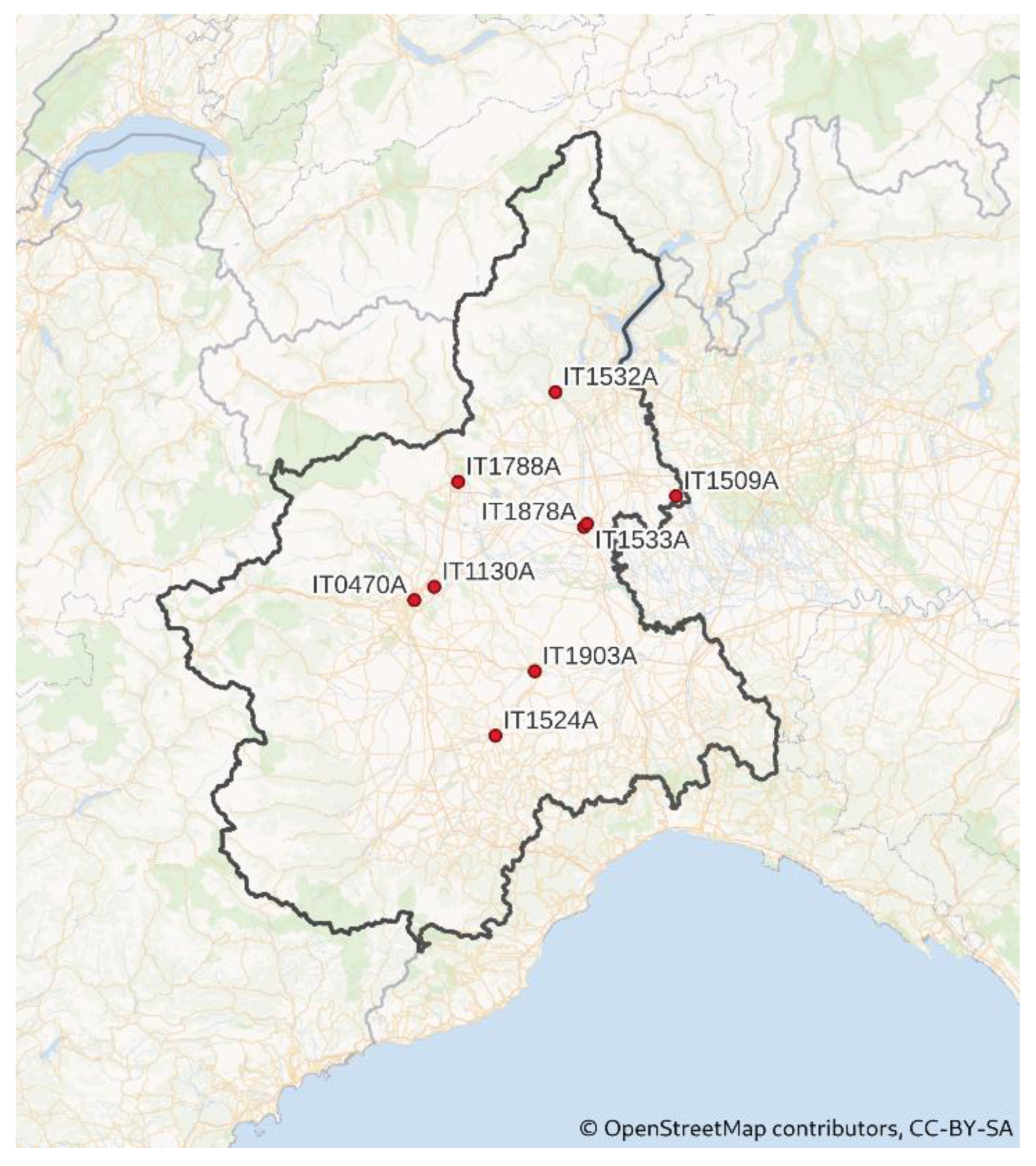
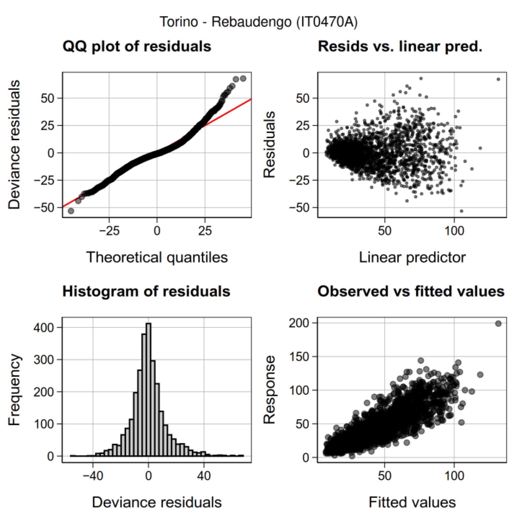
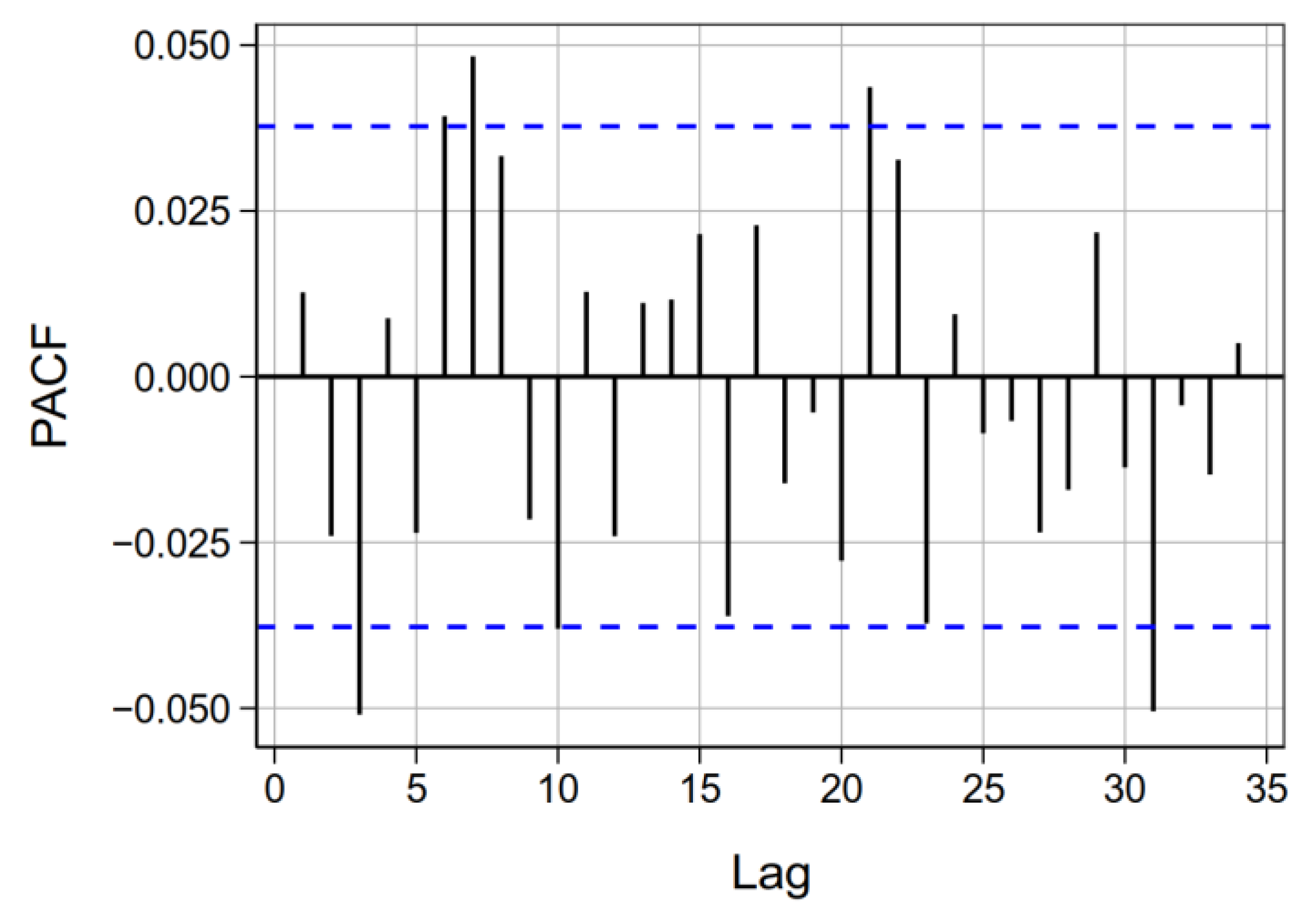
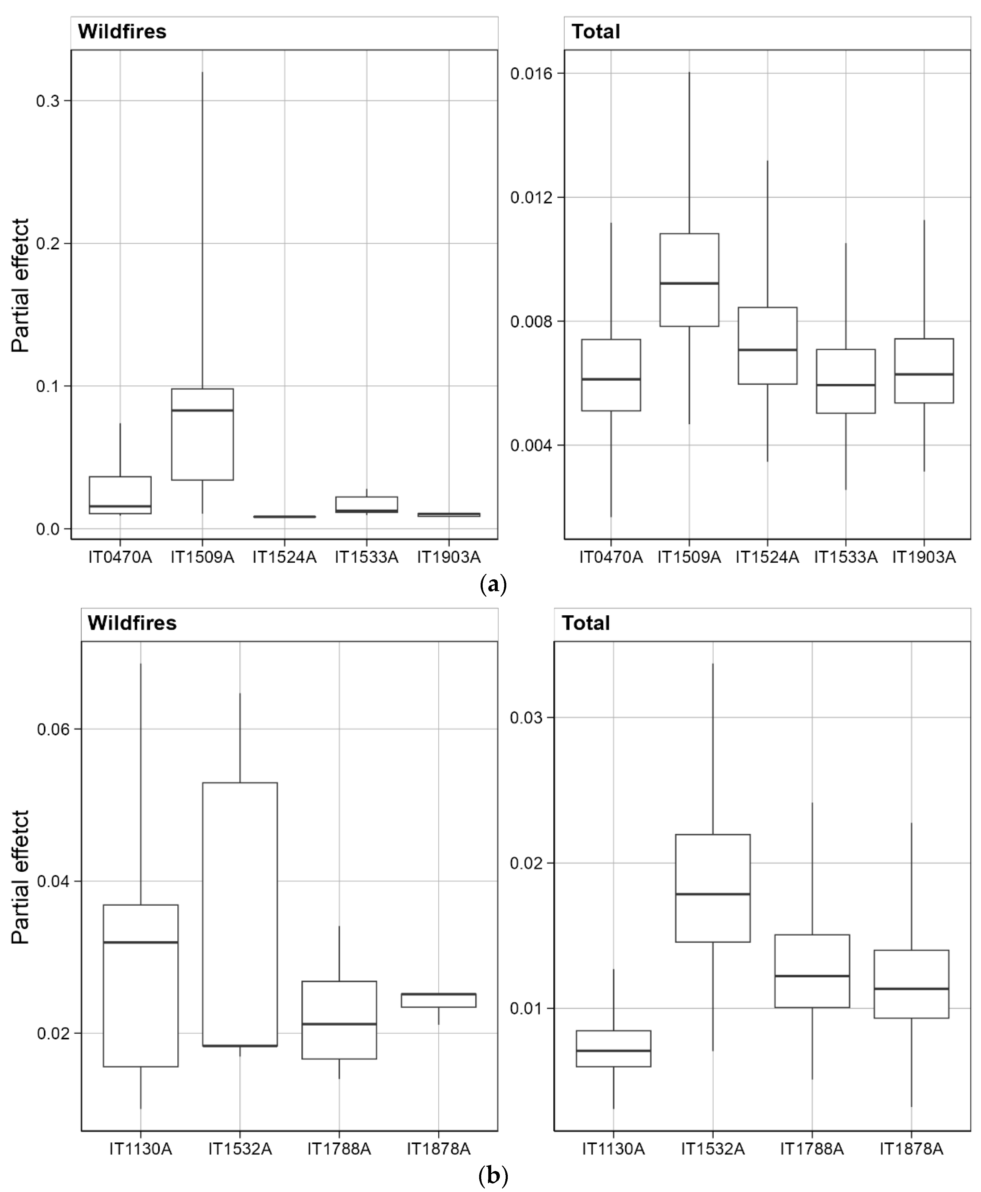
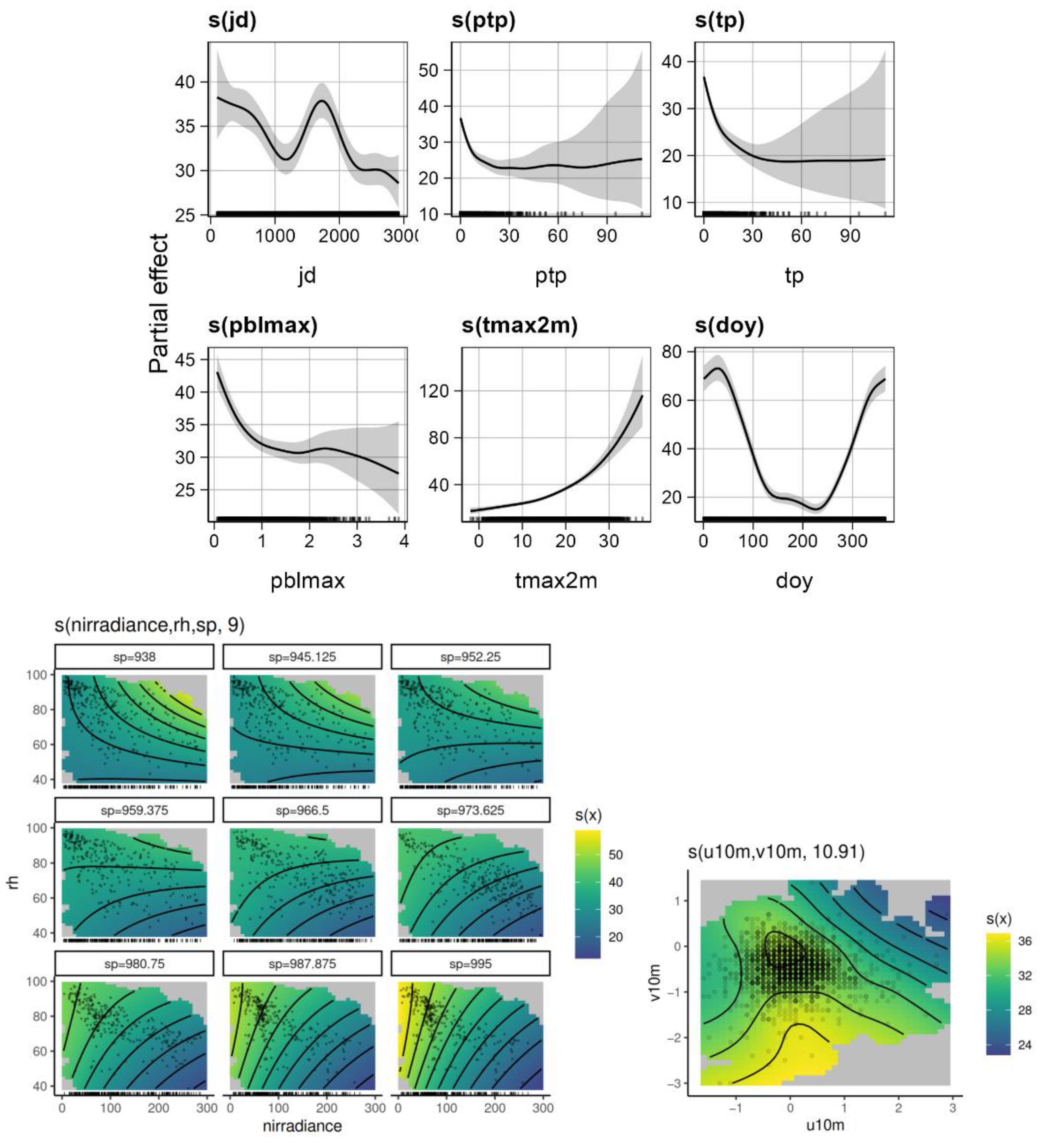
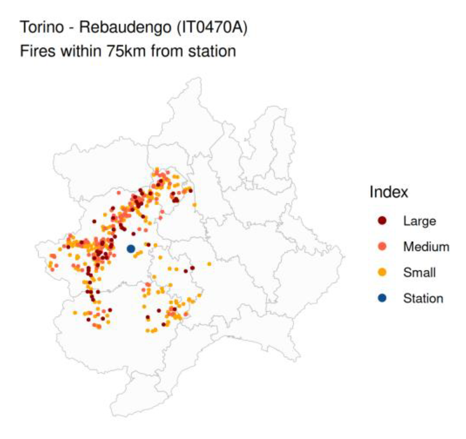
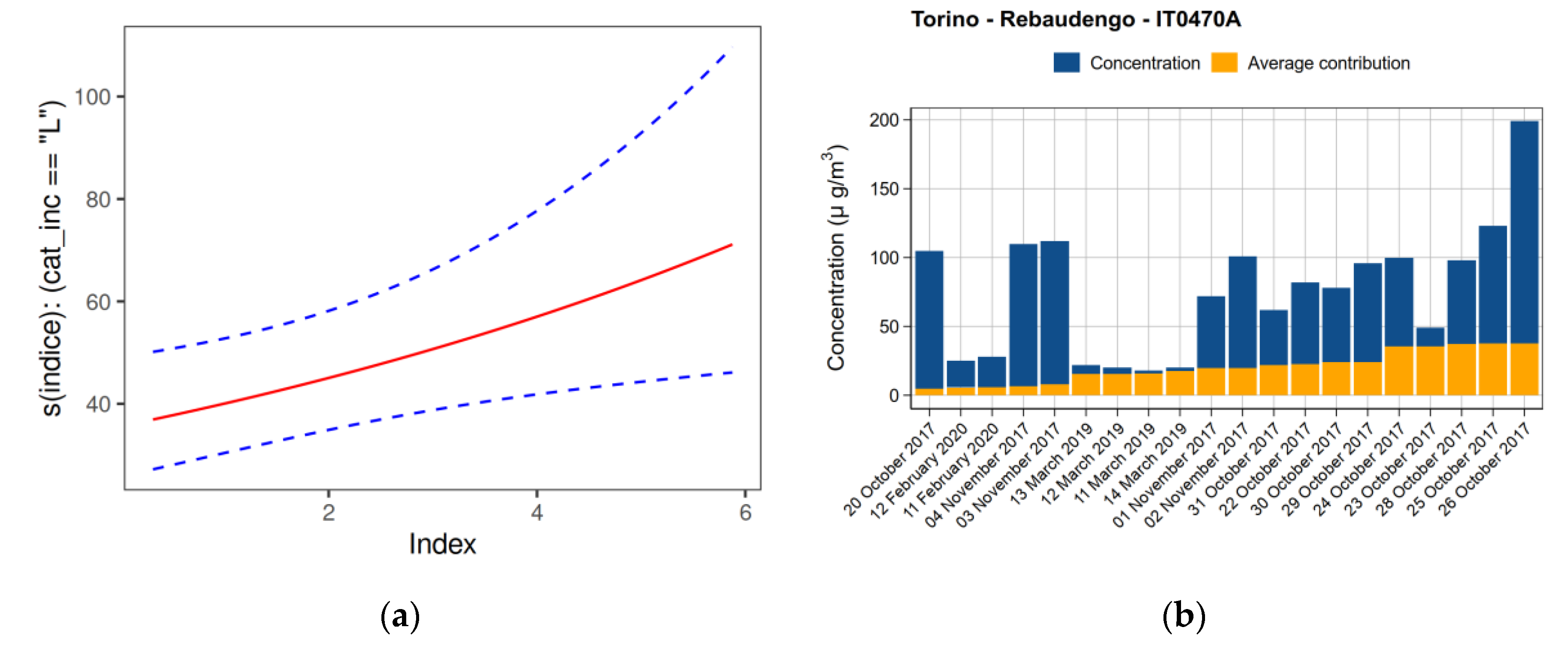
Table 1.
Piedmont air quality monitoring stations information.
| Station Code | Province | Station Name | Longitude (Decimal Degrees) | Latitude (Decimal Degrees) | Altitude (m) |
|---|---|---|---|---|---|
| IT1788A | Torino | Ivrea—Liberazione | 7.87804 | 45.4512 | 240 |
| IT0470A | Torino | Torino—Rebaudengo | 7.69534 | 45.10407 | 23 |
| IT1130A | Torino | Settimo T.—Vivaldi | 7.77818 | 45.1432 | 202 |
| IT1878A | Vercelli | Vercelli—CONI | 8.40236 | 45.31891 | 131 |
| IT1533A | Vercelli | Vercelli—Gastaldi | 8.41514 | 45.32842 | 130 |
| IT1532A | Vercelli | Borgosesia—Tonella | 8.28353 | 45.71317 | 344 |
| IT1509A | Novara | Cerano—Bagno | 8.786132 | 45.40973 | 124 |
| IT1524A | Cuneo | Alba—Tanaro | 8.03328 | 44.70371 | 164 |
| IT1903A | Asti | Asti—Baussano | 8.19756 | 44.89422 | 119 |
Table 2.
Meteorological variables used for the GAMM implementation.
| Name | Temporal Predictors | Unit |
|---|---|---|
| t2m | Mean temperature at 2 m height from ground level | °C |
| tmin2m | Minimum temperature at 2 m height from ground level | °C |
| tmax2m | Maximum temperature at 2 m height from ground level | °C |
| rh | Relative humidity | % |
| tp | Total precipitation | mm |
| ptp | Total precipitation of the previous day | mm |
| u10m | Horizontal component of wind speed at 10 m height (E) | m/s |
| v10m | Vertical component of wind speed at 10 m height (N) | m/s |
| wspeed | Wind speed intensity at 10 m height | m/s |
| pwspeed | Wind speed intensity at 10 m height of the previous day | m/s |
| wdir | Wind direction | Degrees clockwise from North |
| sp | Ground level pressure | hPa |
| nirradiance | Solar radiation intensity | W/mq |
| pbl00 | Planetary boundary layer height at 00:00 | km |
| pbl12 | Planetary boundary layer height at 12:00 | km |
| pblmin | Minimum planetary boundary layer height | km |
| ppblmin | Minimum planetary boundary layer height of the previous day | km |
| pblmax | Maximum planetary boundary layer height | km |
| ppblmax | Maximum planetary boundary layer height of the previous day | km |
Table 3.
(a) PM10 model performance statistics. (b) PM2.5 model performance statistics.
| (a) | |||||
| Station Code | RMSEtrain (RMSEtest) (µg/m3) | R2 train (R2 test) | FAC2 | FB | NMSE |
| IT0470A | 11.43 (11.82) | 0.80 (0.75) | 0.96 | 0.002 | 0.08 |
| IT1509A | 12.68 (12.11) | 0.63 (0.59) | 0.90 | 0.010 | 0.14 |
| IT1524A | 10.62 (11.27) | 0.63 (0.60) | 0.92 | 0.001 | 0.13 |
| IT1533A | 11.74 (11.28) | 0.66 (0.61) | 0.97 | 0.006 | 0.01 |
| IT1903A | 11.80 (11.98) | 0.70 (0.69) | 0.96 | 0.001 | 0.09 |
| - | Acceptability Threshold: >0.5 | Accept. Thresh.: >0.8 | Accept. Thresh.: <0.5 | Accept. Thresh.: <0.5 | |
| (b) | |||||
| Station Code | RMSEtrain (RMSEtest) (µg/m3) | R2 train (R2 test) | FAC2 | FB | NMSE |
| IT1130A | 9.17 (8.59) | 0.83 (0.85) | 0.95 | 0.028 | 0.07 |
| IT1532A | 6.65 (7.68) | 0.67 (0.55) | 0.88 | 0.015 | 0.19 |
| IT1788A | 9.47 (9.63) | 0.71 (0.68) | 0.88 | 0.003 | 0.16 |
| IT1878A | 9.33 (9.32) | 0.70 (0.69) | 0.91 | 0.004 | 0.15 |
| - | Acceptability Threshold: >0.5 | Accept. Thresh.: >0.8 | Accept. Thresh.: <0.5 | Accept. Thresh.: <0.5 | |
Table 4.
Model formula for each station.
| Station Code | Pollutant | Model Formula * | Wildfire Index |
|---|---|---|---|
| IT0470A | PM10 | log(value) ~ s(x)fix + s(ptp) + s(tp) + s(pblmax) + s(tmax2m) + s(index, by =(cat_inc = “L”)) + s(nirradiance, rh, sp) | L |
| IT1509A | PM10 | log(value) ~ s(x)fix + s(ptp) + s(rh) + s(tmax2m) + s(pblmin) + s(index, by = (cat_inc = “M”)) + s(index, by = (cat_inc = “L”)) + s(nirradiance, tmax2m, sp) | M—L |
| IT1524A | PM10 | log(value) ~ s(x)fix + s(ptp) + s(pblmax) +s(tp) + s(sp) + s(index, by = (cat_inc = “L”)) + s(nirradiance, rh, tmax2m) | L |
| IT1533A | PM10 | log(value) ~ s(x)fix + s(ptp) + s(sp) +s(t2m) +s(tmin2m) + s(index, by = (cat_inc = “M”)) + s(index, by = (cat_inc = “L”)) + s(nirradiance, rh, sp) | M—L |
| IT1903A | PM10 | log(value) ~ s(x)fix + s(ptp) + s(pblmax) + s(rh) + s(t2m) + s(index, by = (cat_inc = “L”)) + s(sp, tmax2m, tp) | L |
| IT1130A | PM2.5 | log(value) ~ s(x)fix + s(ptp) + s(pblmax) +s(tp) + s(t2m) + s(nirradiance) + s(pblmin) + s(wspeed_max) + s(index, by = (cat_inc = “M”)) + s(index, by = (cat_inc = “L”)) + s(rh, sp, tmax2m) | M—L |
| IT1532A | PM2.5 | log(value) ~ s(x)fix + s(ptp) +s(t2m) + s(sp) + s(index, by = (cat_inc = “L”)) + s(nirradiance, rh, tmax2m) | L |
| IT1788A | PM2.5 | log(value) ~ s(x)fix + s(pblmax) + s(ptp) + s(t2m) +s(sp) + s(tp) + s(index, by = (cat_inc = “L”)) + s(nirradiance, rh, tmax2m) | L |
| IT1878A | PM2.5 | log(value) ~ s(x)fix + s(ptp) + s(tmax2m) + s(sp) + s(pblmax) + s(tp) + s(u10m) + s(wspeed_max) + s(index, by = (cat_inc = “L”)) + s(nirradiance, rh, tmax2m) | L |
* value = PM daily concentration; s()= spline function; s(x)fix = s(jd) + s(u10m, v10m) + s(doy); cat_inc = wildfire index class.
Table 5.
Summary of qualitative partial effect on PM levels (derived from Figure 5 and Figures S1d–S8d) and number of occurrences of the explanatory variables.
Table 5.
Summary of qualitative partial effect on PM levels (derived from Figure 5 and Figures S1d–S8d) and number of occurrences of the explanatory variables.
| Explanatory Variable | PM10 (n.ocurrences/n.models) | PM2.5 (n.ocurrences/n.models) | Partial Effect PM10 * | Partial Effect PM2.5 * |
|---|---|---|---|---|
| ptp | 5/5 | 4/4 | − − | − − |
| tp | 1/5 | 3/4 | − − | − |
| tmax2m | 2/5 | 1/4 | + + | + + |
| tmin2m | 1/5 | 0/4 | − − | 0 |
| t2m | 1/5 | 2/4 | + + | + − |
| pblmax | 3/5 | 2/4 | − − | - |
| pblmin | 1/5 | 1/4 | − − | − − |
| rh | 2/5 | 0/4 | + + | 0 |
| sp | 2/5 | 3/4 | + | + |
| nirradiance | 0/5 | 1/5 | 0 | − − |
| wspeed_max | 0/5 | 2/4 | 0 | − |
* Qualitative partial effect: (++) = strong increase of PM; (+) = increase of PM; (+ −) = effect not clear; (−) = decrease of PM; (− −) = strong decrease of PM; (0) = null.
Table 6.
Val di Susa wildfire event in IT0470A station: comparison between estimated wildfire PM10 contribution from model and wildfire contribution from speciation, in relation to PM10 measured concentrations.
Table 6.
Val di Susa wildfire event in IT0470A station: comparison between estimated wildfire PM10 contribution from model and wildfire contribution from speciation, in relation to PM10 measured concentrations.
| Date | Observed Value (µg/m3) | Wildfire Contribution from Speciation (µg/m3) min–max | Wildfire Contribution from Model (µg/m3) |
|---|---|---|---|
| 24 October 2017 | 100 | 28.0–36.0 | 35.3 |
| 25 October 2017 | 123 | 34.4–44.3 | 37.8 |
| 26 October 2017 | 199 | 55.7–71.6 | 37.8 |
Disclaimer/Publisher’s Note: The statements, opinions and data contained in all publications are solely those of the individual author(s) and contributor(s) and not of MDPI and/or the editor(s). MDPI and/or the editor(s) disclaim responsibility for any injury to people or property resulting from any ideas, methods, instructions or products referred to in the content. |
© 2023 by the authors. Licensee MDPI, Basel, Switzerland. This article is an open access article distributed under the terms and conditions of the Creative Commons Attribution (CC BY) license (https://creativecommons.org/licenses/by/4.0/).
Share and Cite
MDPI and ACS Style
Leone, G.; Cattani, G.; Cusano, M.; Gaeta, A.; Pellis, G.; Vitullo, M.; Morelli, R. Wildfires Impact Assessment on PM Levels Using Generalized Additive Mixed Models. Atmosphere 2023, 14, 231. https://doi.org/10.3390/atmos14020231
AMA Style
Leone G, Cattani G, Cusano M, Gaeta A, Pellis G, Vitullo M, Morelli R. Wildfires Impact Assessment on PM Levels Using Generalized Additive Mixed Models. Atmosphere. 2023; 14(2):231. https://doi.org/10.3390/atmos14020231
Chicago/Turabian StyleLeone, Gianluca, Giorgio Cattani, Mariacarmela Cusano, Alessandra Gaeta, Guido Pellis, Marina Vitullo, and Raffaele Morelli. 2023. "Wildfires Impact Assessment on PM Levels Using Generalized Additive Mixed Models" Atmosphere 14, no. 2: 231. https://doi.org/10.3390/atmos14020231
Note that from the first issue of 2016, this journal uses article numbers instead of page numbers. See further details here.