Article

Decadal Application of WRF/Chem under Future Climate and Emission Scenarios: Impacts of Technology-Driven Climate and Emission Changes on Regional Meteorology and Air Quality

1
Department of Marine, Earth, and Atmospheric Sciences, North Carolina State University, Raleigh, NC 27695, USA
2
India Meteorological Department, Ministry of Earth Science, Lodhi Road, New Delhi 110003, India
3
Department of Civil and Environmental Engineering, Northeastern University, Boston, MA 02115, USA
4
Lynker, Environmental Modeling Center, NOAA, College Park, MD 20740, USA
5
Cooperative Institute for Satellite Earth System Studies, Center for Spatial Information Science and Systems, George Mason University, Fairfax, VA 22030, USA
6
Atmospheric Sciences Modeling Division, Air Resources Laboratory, NOAA, College Park, MD 20740, USA
*
Author to whom correspondence should be addressed.
Atmosphere 2023, 14(2), 225; https://doi.org/10.3390/atmos14020225
Submission received: 9 December 2022 / Revised: 12 January 2023 / Accepted: 16 January 2023 / Published: 21 January 2023
(This article belongs to the Section Air Quality)

Abstract

:
This work presents new climate and emissions scenarios to investigate changes on future meteorology and air quality in the U.S. Here, we employ a dynamically downscaled Weather Research and Forecasting model coupled with chemistry (WRF/Chem) simulations that use two Intergovernmental Panel on Climate Change scenarios (i.e., A1B and B2) integrated with explicitly projected emissions from a novel Technology Driver Model (TDM). The projected 2046–2055 emissions show widespread reductions in most gas and aerosol species under both TDM/A1B and TDM/B2 scenarios over the U.S. The WRF/Chem simulations show that under the combined effects of the TDM/A1B climate and emission changes, the maximum daily average 8-h ozone (MDA8 h O3) increases by ~3 ppb across the U.S. mainly due to widespread increases in near-surface temperature and background methane concentrations, with some contributions from localized TDM emission changes near urban centers. For the TDM/B2 climate and emission changes, however, the MDA8 h O3 is widely decreased, except near urban centers where the relative TDM emission changes and O3 formation regimes leads to increased O3. The number of O3 exceedance days (i.e., MDA8 h O3 > 70 ppb) for the entire domain is significantly reduced by a grid cell maximum of up to 43 days (domain average ~0.5 days) and 62 days (domain average ~2 days) for the TDM/A1B and TDM/B2 scenarios, respectively, while in the western U.S., larger O3 increases lead to increases in nonattainment areas, especially for the TDM/A1B scenario. The combined effects of climate and emissions (for both A1B and B2 scenarios) will lead to widespread decreases in the daily 24-h average (DA24 h) PM2.5 concentrations, especially in the eastern U.S. (max decrease up to 93 µg m−3). The PM2.5 changes are dominated by decreases in anthropogenic emissions for both the TDM/A1B and TDM/B2 scenarios, with secondary effects on decreasing PM2.5 from climate change. The number of PM2.5 exceedance days (i.e., DA24 h PM2.5 > 35 µg m−3) is significantly reduced over the eastern U.S. under both TDM/A1B and B2 scenarios, which suggests that both climate and emission changes may synergistically lead to decreases in PM2.5 nonattainment areas in the future.

1. Introduction

Rapid and complex increases in population and economy lead to changes in weather, climate, and air quality. Use of emission projections in gridded atmospheric climate and chemistry models are critical elements in the understanding of future climate impacts on regional air quality. There are two popular sets of emission scenarios developed by the Intergovernmental Panel on Climate Change (IPCC) research community, both of which are based on expert judgments of plausible future emissions that consider socioeconomic, environmental, and technological trends: (1) the “Special Report on Emissions Scenarios” (SRES) [1], and (2) the “Representative Concentration Pathways” (RCP) [2].
The SRES scenarios represent a “big-picture” approach that covers a wide range of main driving forces of future emissions based on demographic, technological, and economic developments. The SRES scenarios are derived from extensive assessment of the literature, six alternative modeling approaches, and an “open process” that solicited wide participation and feedback from expert groups and individuals [1]. We note that there are no future policies that address climate change in the SRES scenarios, and that they include a range of emissions of all relevant species of greenhouse gases (GHGs) and sulfur. Unlike the SRES, the RCP scenarios are based on the concept of four scenarios of future radiative forcing pathways (i.e., an atmospheric response of changing incoming vs. outgoing radiation due to changes in atmospheric GHGs, such as carbon dioxide) that can be achieved by a diverse range of socioeconomic and technological development scenarios [2].
Using SRES scenarios, many studies have investigated the effect of future changes in climate and anthropogenic emissions on air quality [3,4,5,6,7,8,9]. It has been found that over the contiguous U.S. (CONUS), potentially large decreases in surface ozone (O3) are simulated when reductions in precursor anthropogenic emission estimates are accounted for, partially counteracting potential increases due to climate change [7,10,11]. For example, Lam et al. (2011) found a 2 to 5 ppbv increase for maximum daily average 8-h ozone (MDA8) O3 in the 2050s compared with the 2000s in the eastern U.S. due to climate changes under the SRES A1B scenario, while maintaining anthropogenic emissions at the 2000s level; however, when accounting for changes in both climate and emissions by 2050, there was an up to ~5 ppbv decrease in MDA8 O3 [7]. Penrod et al. (2014) further analyzed the combined climate and anthropogenic emission changes under the SRES A1B scenario and showed that increased future temperatures lead to increases in O3 of up to ~5 ppbv in winter for the eastern U.S., but that widespread anthropogenic emission decreases of nitrogen oxides (NOx) lead to larger reductions of O3 of up to ~12 ppbv in summer over most of the U.S. by 2026–2030 [12]. Overall, the consensus of these SRES-based studies tends to indicate an agreement in future (short term by ~2030 and long-term by ~2050) widespread decreases in O3 over CONUS when both climate effects and declining anthropogenic emissions are accounted for, where the O3 changes are typically dominated by changes in emissions. There is, however, clear spatiotemporal variability in the amount and direction of change throughout these SRES studies on O3 (e.g., some rising O3 levels near urban regions), which are confounded by potentially rising GHG concentrations (e.g., methane, CH4) that are also important to O3 formation. While not detailed here, there is further uncertainty and spread across the SRES-based studies on the impacts of climate and emissions on future fine particulate matter (PM2.5) concentrations over CONUS; however, we note that Penrod et al. (2014) found that anthropogenic emission reductions dominate future PM2.5 decreases across the U.S., with a secondary effect of increased precipitation and wet deposition from future near-term (2030) climate impacts [12].
Many studies have also investigated the impacts of projected emission and climate changes on air quality under the RCP scenarios [13,14,15,16,17,18,19,20,21]. Pfister et al. (2014) used a regional coupled chemistry-transport model under the RCP8.5 scenario and showed that future regional climate and globally enhanced background ozone will lead to increased surface O3 by 2050 over most of the U.S.; however, they noted that pronounced differences across the U.S. could not be resolved at the coarse resolution of the model used and that future stringent emission controls can counteract these increases [18]. Yahya et al. (2017) used the regional, online-coupled Weather Research and Forecasting model coupled with chemistry (WRF/Chem) in conjunction with climate and explicit anthropogenic emission changes over the U.S. to show that future O3 mixing ratios show decreases of ~2 ppbv by ~ 2050 under the RCP4.5 scenario, except for major urban cities in California and in the northeastern U.S. [22,23]. However, under the RCP8.5 scenario, Yahya et al. (2017) also showed there was an increase of ~3 ppbv over all parts of the U.S. by 2050, which is driven by higher GHG and biogenic volatile organic compounds (BVOCs) [23]. These results of increasing O3 due to climate and increasing BVOCs are similar to those of Pfister et al. (2014) for the RCP8.5 scenario [18]. Yahya et al. also found that the PM2.5 concentration will decrease over CONUS for both the RCP scenarios [23]. Nolte et al. (2018) showed the impacts of downscaled climate and anthropogenic emission changes on U.S. air quality for three RCP scenarios, and that the MDA8 O3 is projected to increase during summer and autumn in the central and eastern U.S., with the largest increases (up to 4 ppb) for the RCP8.5 scenario by 2030 [20]. Nolte et al. also reported mixed PM2.5 changes, with annual average PM2.5 concentration ranges from −1.0 to 1.0 µg m−3 over CONUS by 2030 [20]. Overall, the RCP-based studies tend to agree that rising temperatures and background GHG concentrations and their contribution to potentially enhanced future O3 formation, particularly during the photochemical O3 formation season in the U.S. These studies also show that climate changes may outweigh the benefits of decreasing anthropogenic emission precursors; however, mainly all studies rely on “big-picture” scenarios and demonstrate uncertainty in how well they can explicitly represent future anthropogenic emission controls, particularly projected technological changes at finer scales. We also note that in all previous studies (and our work here), there is uncertainty from neglecting future land use/vegetation change on the sources and sinks of O3/PM2.5 and predicted changes.
We note that the SRES were developed prior to the RCP projections and show definitive differences in their impacts on future regional air quality as described in the aforementioned studies. Furthermore, Rogelj et al. (2012) showed that there are uncertainties in the projections of both the IPCC SRES and RCP scenarios, and there are both similarities and differences between the scenario families [24]. There is evidence that shows a weakness of the SRES, because there are no “real-world” technological mitigation policies implied in any SRES scenario [1], and that the RCP scenarios have simply evolved from the SRES in a similar manner. The RCP scenarios themselves are also not fully integrated scenarios (i.e., they are not a complete package of socioeconomic, emissions, and climate projections), and thus there is validity in continuing to apply and investigate the impacts of the SRES-based projections in conjunction with more explicitly developed anthropogenic emission inventories at finer scales, as in this work for the U.S.
The emission projections in the aforementioned SRES- and RCP-based studies do not account for detailed, explicit relationships between future socioeconomic factors and projected technology changes, but rather only by expert judgments. Consequently, Yan et al. (2014) developed an advanced Technology Driver Model (TDM), which links socioeconomic factors and projected technology change [25]. The TDM more accurately differentiates emitters by their emission characteristics that are continually influenced by dynamic changes in technology (i.e., economic development, policy changes, and emission control strategies), while determining the emission factors using explicit relationships rather than by expert judgments [25,26]. Campbell et al. (2018) investigated impacts of projected transportation sector-only emissions on air quality based on the TDM approach at the U.S. state-level [26,27]. They found that future O3 mixing ratios would decrease if only considering emission changes and would increase when considering both emission and climate change (in conjunction with increasing GHG, e.g., CH4 concentrations).
The spatial, temporal, and socioeconomic-technological relationship variabilities in future emission projections can have important impacts on the predicted future air quality changes, especially when combined with climate change impacts. Socioeconomic aspects of the SRES scenarios alone include different human population growth trajectories based on published projections [1]. For example, the SRES “A1” scenario is based on low population growth trajectories up to 8.7 billion people by the year 2050, and then decreasing toward 7 billion by 2100. The “B2” scenario, however, applies a long-term increasing population projection of up to 10.4 billion by the year 2100 [1]. The use of such SRES scenarios alone ignores other critical details of the combined interactions of socioeconomic–technological relationships that affect such trajectories, and thus, the TDM approach, to some extent, overcomes the aforementioned limitations in SRES- and RCP-based projections used with similarly predicted anthropogenic emissions for the U.S.
In this work, we expand upon previous work [26,27] and apply the emissions projected by the TDM approach for all major anthropogenic emission sectors (i.e., transportation, power plant, industrial, and residential sectors) at the U.S. state-level under two SRES scenarios (i.e., A1B and B2). Here, we dynamically downscale the global Community Earth System Model/Community Atmosphere Model (CESM/CAM5) simulations to provide the initial and boundary conditions for the regional, online-coupled WRF/Chem model. We use the TDM approach and the downscaled regional WRF/Chem simulations to investigate the individual and combined impacts of climate change and emission projections on the future regional air quality over CONUS during current (2001–2010) and future (2046–2055) decades.

2. Model Description and Simulation Setup

Table 1 summarizes six decadal simulations that are performed using the WRF/Chem v3.7 model [28]. Two sets of baseline simulations are performed: one with the best possible emissions of 2001–2010 based on the U.S. EPA National Emissions Inventory (NEI) 2002, 2005, and 2008 (BASE_EVAL) for model performance evaluation, and one with the TDM baseline 2005 emissions during the SRES current climate period of 2001–2010 (BASE_TDM) that serves as the reference for simulations with projected emission changes. Two additional simulations are performed under the current 2001–2010 climate with future 2046–2055 projected TDM emissions (Table 1; EMIS_A1B and EMIS_B2). Comparing these two simulations with the TDM baseline 2005 simulation (i.e., climate held constant) allows for quantifying the impacts of TDM emission changes only. Two additional simulations are performed under the future 2046–2055 climate (SRES A1B and B2) with future 2046–2055 projected TDM emissions (CLIM_EMIS_A1B and CLIM_EMIS_B2). Comparing these two simulations with the BASE_TDM (with baseline TDM 2005 emissions and current 2001–2010 climate) allows for quantifying the impacts of both emissions and climate changes. Comparing these two simulations with those for the 2001–2010 climate with future 2046–2055 projected TDM emissions (i.e., emissions held constant) allows for quantifying the impacts of climate changes only (CLIM_ A1B and CLIM_ B2, which are also included in Table 1).
Wang et al. (2021) previously described and evaluated the same WRF/Chem v3.7 model for a baseline evaluation 2001–2010 period over CONUS (Table 1; BASE_EVAL) [29]. Therefore, the results of Wang et al. will not be repeated here; however, we note that the BASE_EVAL WRF/Chem simulations showed good performance for major meteorological and chemical variables compared with the literature [29]. Wang et al. further discussed the potential WRF/Chem model biases that may lead to uncertainties in the future air quality projections presented in our work [29].
The WRF/Chem simulation domain covers CONUS and parts of Canada and Mexico, with a horizontal resolution of 36 km with 148 × 112 horizontal grid cells, and a vertical resolution of 34 layers from the surface to 100 mb. The physics options include the Rapid Radiative Transfer Model for GCMs (RRTMG) for shortwave (SW) and longwave (LW) radiation, the Yonsei University (YSU) scheme for planetary boundary layer (PBL), the Noah Land Surface Model (LSM), the Morrison double moment scheme for microphysics, and the Multi-Scale Kain Fritsch (MSKF) scheme for the cumulus parameterization (Table 2).
The major chemistry options include the extended Carbon Bond 2005 (CB05) gas-phase mechanism with updated chlorine chemistry and the Modal for Aerosol Dynamics in Europe (MADE) aerosol module coupled with an advanced secondary organic aerosol (SOA) treatment, i.e., the Volatility Basis Set (VBS) module (Table 2). The coupled CB05-MADE/VBS option has also been linked with existing model treatments of various feedback processes such as the aerosol semi-direct effect on photolysis rates of major gases, and the aerosol indirect effect on cloud droplet number concentration (CDNC) and resulting impacts on shortwave radiation [51].
The anthropogenic emissions for current years (2001–2010) are based on U.S. EPA NEI) emission versions 2002, 2005, and 2008 that cover the 10-year time period (Table 2). Future emissions are projected to 2046–2055 using the growth factors (from the 2005 base year) generated by the TDM model based on the approach described below in Section 3. Biogenic emissions are calculated online using the Model of Emissions of Gases and Aerosols from Nature version 2 (MEGAN2) [47]. Dust and sea salt emissions are generated online using the Atmospheric and Environmental Research Inc. and Air Force Weather Agency (AER/AFWA) scheme [48,49] and the Gong et al. (1997) scheme [50], respectively (Table 2).
The chemical and meteorological initial/boundary conditions (ICONs/BCONs) are generated following a previously described dynamic downscaling technique [22,23] using global simulations from the modified CESM/CAM5 version 1.2.2 [45,52]. In addition to similar gas-phase chemistry and aerosol treatments, the CESM/CAM5 and WRF/Chem simulations both use the RRTMG for shortwave and longwave radiation schemes, but do have different cloud microphysics, PBL, and convection schemes. Furthermore, the CESM/CAM5 default LSM is the Community Land Model (CLM; https://www.cesm.ucar.edu/models/clm/ (accessed on 18 November 2022)) in CESM/CAM5, and here we use the Noah LSM in WRF/Chem. As global climate models (GCMs) generally contain systematic biases for meteorology that can influence the downscaled simulations, the meteorological ICONs/BCONs are bias-corrected before they are used in the WRF/Chem simulation using a simple bias correction technique [22,23,53]. This bias correction technique is also applied for future year simulations. Considering the decadal applications of WRF/Chem in this work, the simulations are reinitialized monthly to constrain meteorological fields while allowing chemistry-meteorology feedbacks within the system. More details on model configurations can be found in Table 2. For a visual flowchart that illustrates the TDM and dynamical downscaling model simulation setup, please see the Graphical Abstract of Campbell et al. (2018) [27].

3. Technology Driver Model (TDM) for Emission Projections

Emission projections are critical elements in understanding future climate impacts at global and regional scales. One of the deficiencies for many current emission projections [1] is the lack of a clear or explicit relationship between socioeconomic factors and projected technology change. Thus, the TDM approach [25,26,27,54] has been developed to help close the gap between socioeconomic factors and projected technology change. This model is based on the Speciated Pollutant Emission Wizard (SPEW)-Trend model [54], which is a hybridization of engineering (“bottom-up”) and economic (“top-down”) models. Yan et al. (2011, 2014) described how the mix of technologies is determined dynamically by deriving explicit relationships among socioeconomic factors and technological changes [25,54]. The SPEW-Trend model is driven by variables taken from IPCC SRES (e.g., A1B and B2), including fuel consumption, population, and gross domestic product. SPEW-Trend determines the final emission projections of the major anthropogenic transportation, power plant, industrial, and residential sectors. The projected emission growth factors are further apportioned to each U.S. state for all anthropogenic emission sectors by their current and future energy consumption data, which is derived from business-as-usual trends reported in the Department of Energy’s 2013 Annual Energy Outlook [55]. Consequently, the growth factors used here are specific to each U.S. state and IPCC emission projection scenario, and thus are highly detailed compared with other emission projection methods and applications. Further details on the SPEW-Trend model and emission projection factors used here may be found in previous work [25,26,54].
Figure 1 shows the absolute differences between future and current carbon monoxide (CO), sulfur dioxide (SO2), nitrogen oxides (NOx), and volatile organic compound (VOC) emissions under the TDM/A1B and TDM/B2 scenarios. Supplementary Figure S1 shows the relative percent changes for the same species, and Supplementary Figures S2 and S3 show both the absolute and relative percent changes for gaseous ammonia (NH3) and particulate elemental carbon (EC), sulfate (SO42−), and total PM2.5.
Overall, there is a reduction of emissions for most gas and aerosol species under both TDM/A1B and TDM/B2 scenarios. Under the TDM/A1B scenario, the emissions of CO, NOx, SO2, and VOCs are reduced near the high population density regions, power plants, and highways and major roads, but slightly increased along coastlines due to shipping emissions. On a domain-wide average, the future TDM/A1B CO, NOx, SO2, and VOC emissions decrease by about 3%, 19%, 20%, and 5%, respectively (Figure S1). For the same emissions species, the TDM/B2 decreases are similar in spatial distribution to TDM/A1B, but have a larger average decrease at about 25%, 38%, 31%, and 16%, respectively (Figure S1). The NOx and SO2 emissions, however, show local increases near the Ohio River and the northern border of Ohio and Lake Erie due to transportation sectors (specifically shipping) under both the scenarios [25,26]. There are increases in CO and VOC emissions in parts of Florida due to on-road sectors under the TDM/A1B scenario [26]. There are also widespread decreases in NH3 emissions for both the TDM/A1B and TDM/B2 scenarios, with domain-wide average decreases of about 5% and 8%, respectively (Figures S2 and S3).
For the particulate matter (PM) species, there are decreases in EC, SO42−, and PM2.5 emissions across the CONUS, but more dominating increases are found in major waterways including the Ohio River and Lake Erie, Mississippi River, and near shipping ports along the west coast, east coast, and the Gulf of Mexico (Figures S2 and S3). Increases in shipping emissions of PM are further elucidated in the relative % differences for regions just off the Pacific Coast and Atlantic Oceans, and the Gulf of Mexico. Overall, on a domain-wide average, the TDM/A1B (TDM/B2) emission changes for EC, SO42−, and PM2.5 are about −11% (−21%), +3% (+1%), and +4% (+2%), respectively (Figures S2 and S3).

4. Impacts of TDM/A1B and TDM/B2 on Future Climate, Clouds, and Air Quality

The following subsections show results from the CLIM_EMIS–BASE_TDM simulations (Table 1), which are used to investigate the combined climate and emission impacts of the TDM/A1B and TDM/B2 scenarios on climate, clouds, and air quality between the future (2046–2055) and current (2001–2010) decades.

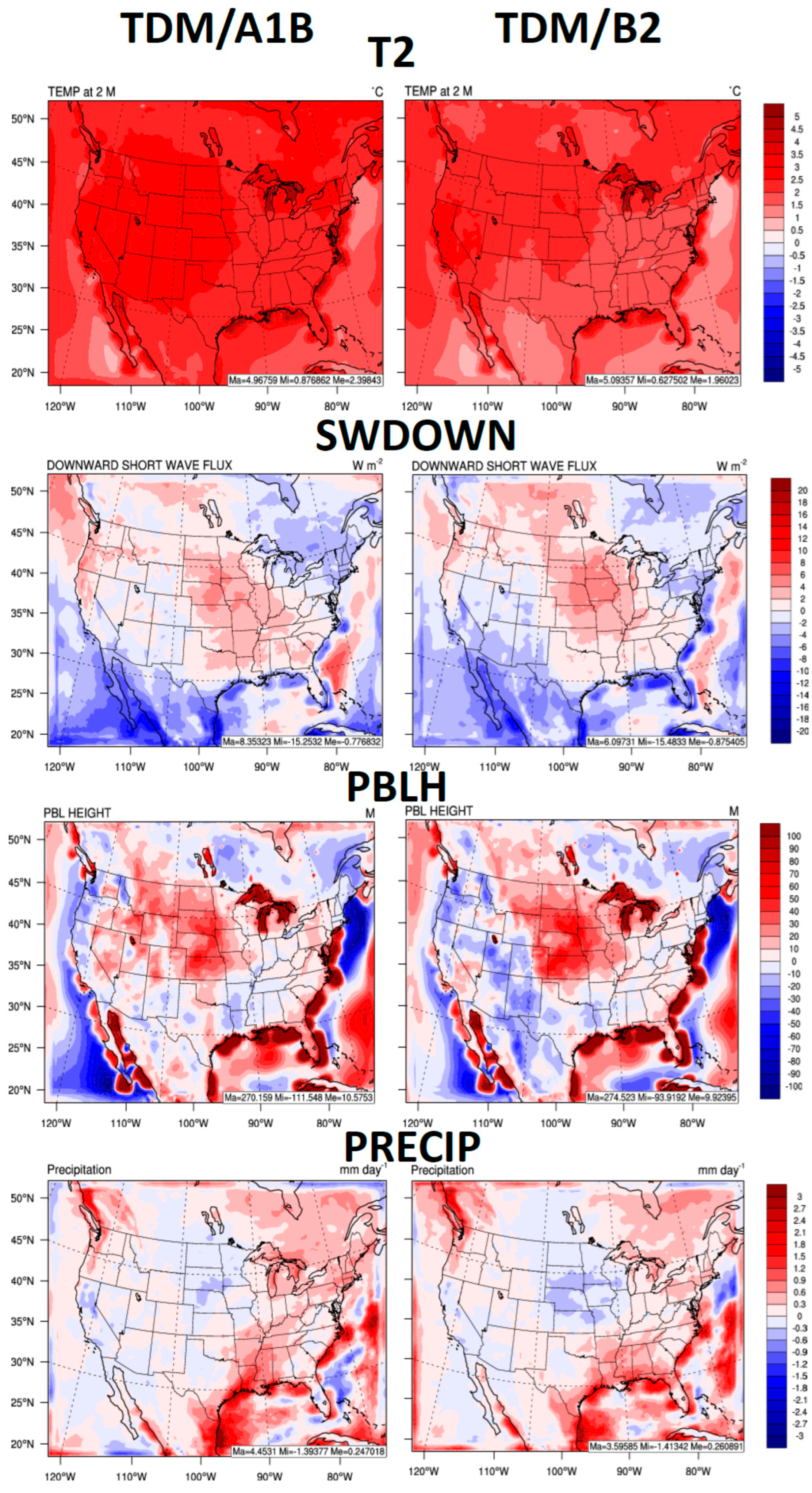
4.1. Impacts on Climate Variables

For the TDM/A1B scenario, the domain-average 2-m temperature (T2) increases by ~2.3 °C (up to a max grid cell increase of ~5.0 °C), where the largest relative increases are in the western and central U.S. and parts of Canada due to increasing greenhouse gases and downward shortwave radiation (SWDOWN) reaching the ground (Figure 2).
Other studies based on RCP scenarios have found differences in the future warming patterns over the CONUS. For example, Yahya et al. (2017) used a downscaled regional WRF-Chem model and showed warmer areas of the north-central U.S. during the future years (2046–2055) compared to current years (2001–2010) [23]. Nazarenko et al. (2015) and Separovic et al. (2013) showed warmer areas in Canada, the central U.S., the north-central U.S., and the western U.S. during the late 21st century [56,57].
The changes in 2-m water vapor mixing ratio (Q2) between the future and current climate closely follow the pattern for changes in T2 (see Supplementary Figure S4). The largest increases in Q2 occur near the coastal areas, and the changes gradually decrease inland. The 10-m wind speeds (WS10) increase over most parts of the U.S. due to the increase in T2, with larger increases near the coastal areas (Figure S4). Planetary boundary layer height (PBLH) increases over most parts of the U.S. due to the increase in T2 and WS10 (Figure 2). The general increase in WS10 over the eastern and southeastern U.S. is consistent with an increase in precipitation (PRECIP) and PBLH over the region (Figure 2), suggesting an increased frequency of Atlantic storms due to increased surface heating and warmer sea surface temperatures (especially near the coastlines). This is consistent with recent work that shows extreme Atlantic hurricane seasons are twice as likely due to ocean warming [58].
The changes in PRECIP show a similar trend to those in Q2, i.e., the largest increases in PRECIP occur over the ocean and near the coastal areas, while for the central U.S., there is a decrease in PRECIP. The decrease in PRECIP here is associated with warmer but drier conditions (less increases and some decreases in Q2; Figure S4), which lead to increases in clear skies and consequently less cloud formation. The drier and clearer skies over the central CONUS is consistent with an increasing trend in outgoing longwave radiation at the top of the atmosphere (OLR) over land ~1.3 W m−2 (Figure S4), which is similar to the study by Yahya et al. (2017) [23].
Ultimately, increases in GHGs in the future scenario lead to overall warming and an ability of the atmosphere to hold more water vapor (i.e., the Clausius–Clapeyron effect). This leads to a dichotomy in the impacts over land vs. ocean, where over land, the warming leads to more evaporation and a drying feedback due to limited evaporation of water vapor from soils, reductions in cloud formation, and an increase in SWDOWN (Figure 2). The increase in SWDOWN over land is relatively large and up to 4 W m−2 (Figure 2). However, the warming over the oceans and evaporation of a relatively unlimited supply of water vapor drive an increase in clouds and storms and a decrease in SWDOWN (i.e., driving the domain-wide decrease at ~0.7 W m−2).
For the TDM/B2 scenario, the domain average T2 increases by ~2 °C with grid cell maximum T2 increases by 5.1 °C, mainly over the north-east-central and east-coast U.S. (Figure 2). The spatial pattern of T2 for TDM/B2 is similar to TDM/A1B, but with lesser increases in eastern and southern U.S. compared with TDM/A1B. The spatial changes of Q2 are also similar to TDM/A1B (Figure S4); however, there are smaller increases in Q2 under TDM/B2 compared with TDM/A1B due to the smaller increases in T2 (i.e., less water vapor holding capacity). The largest increases in WS10 occur in coastal areas of the U.S. and central Canada and are associated with correlated increases in T2. We note that there are also very small decreases in WS10 in the western and central U.S. (Figure S4). The large increases in PBLH over the central and coastal regions of the U.S. are due to increases in T2 and WS10, with small decreases in PBLH in western and southwestern U.S. (Figure 2). In general, the increased WS10, PRECIP, and PBLH also suggest an increased frequency of Atlantic storms in the TDM/B2 scenario. The changes in PRECIP also show a similar trend to the changes in Q2, i.e., the largest increases in precipitation occur over the ocean and near the coastal areas, while for the central U.S., there is a decrease in precipitation (Figure 2). The spatial pattern of PRECIP for TDM/B2 is similar to TDM/A1B. This trend is similar to the results from previous studies using the RCP scenarios, which also show the largest increase in PRECIP over the southeastern U.S. [13,23] There is a domain-wide decrease in SWDOWN of ~0.9 W m−2 but a much larger increase in SWDOWN of about 0 to 4 W m−2 over the central U.S. The SWDOWN is projected to increase over the central U.S. due to increase in GHGs leading to overall warmer T2, deeper PBLHs, smaller (or decreased) Q2, and reduced cloud formation feedbacks from aerosol reductions over these inland regions (see Section 4.4 for more discussion). The trend for OLR is also similar to TDM/A1B with an increase over land by ~1.3 W m−2 (Figure S4). The downward longwave radiation (not shown) increases with a domain average of ~11.0 W m−2 due to increases in GHGs in the future scenario.

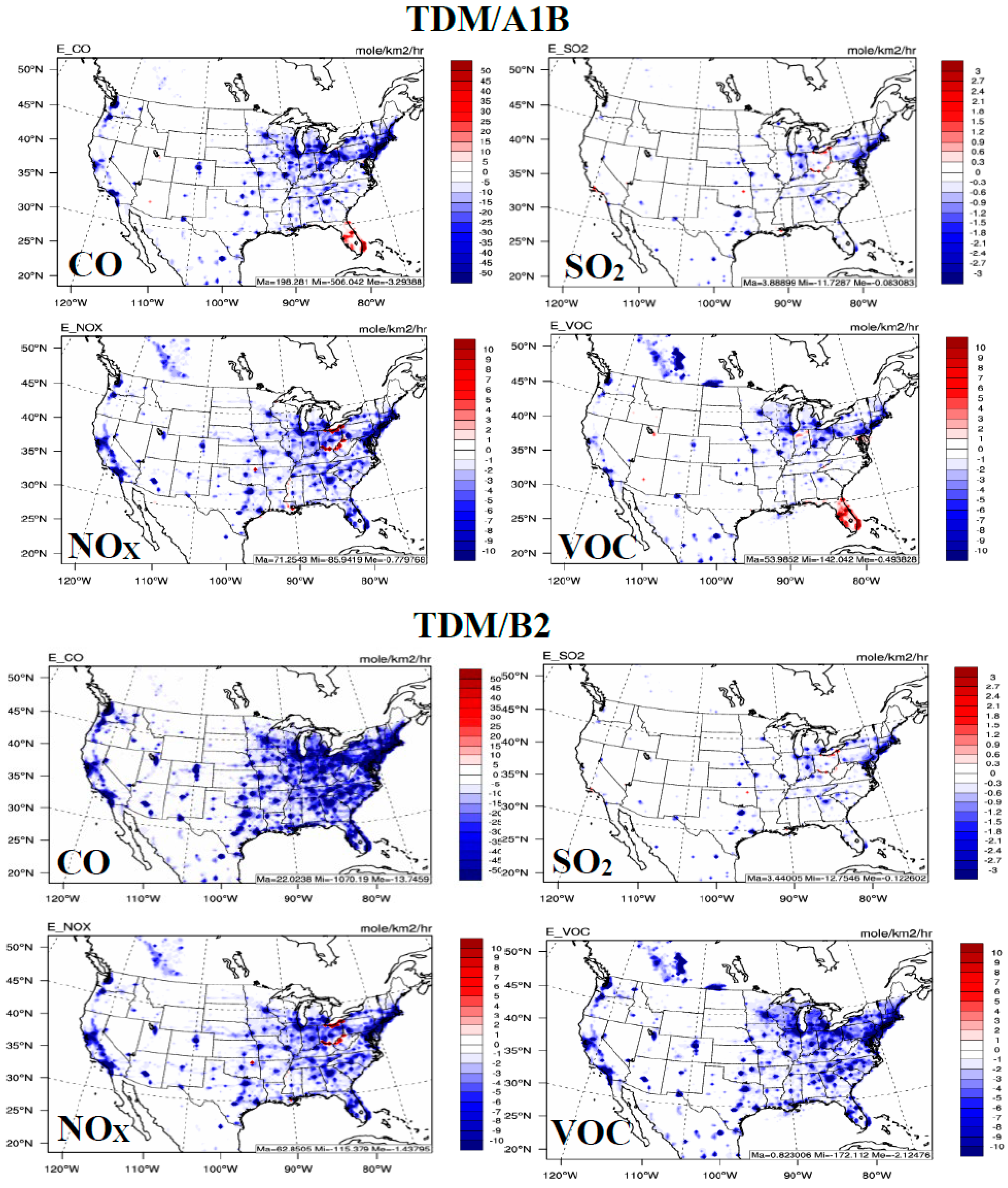
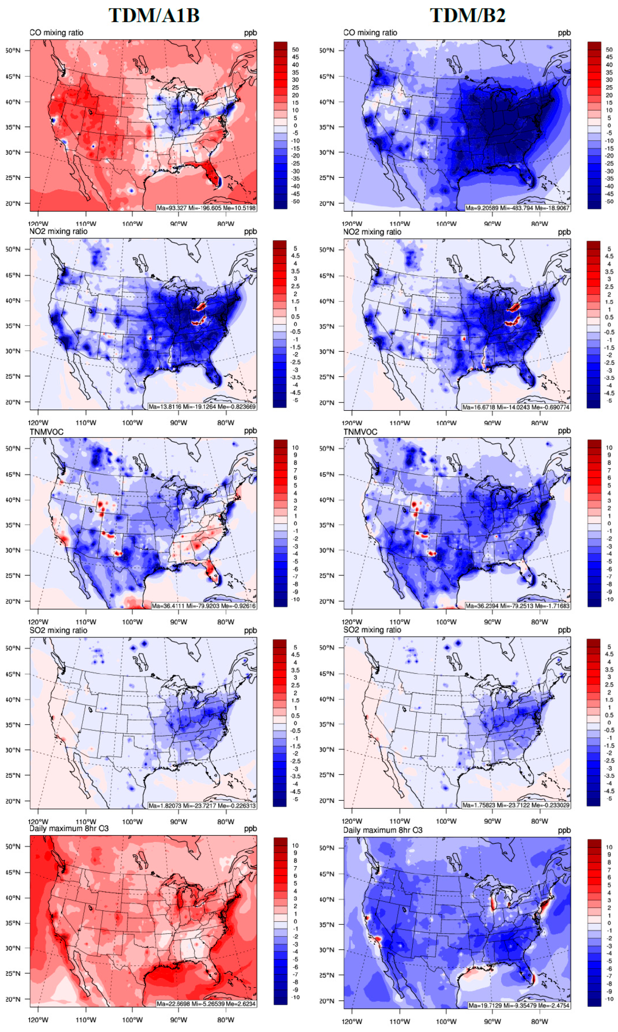
4.2. Impacts on Air Quality Variables

The mixing ratio of NO2 is projected to decrease for both TDM/A1B (ave. ~0.8 ppb) and TDM/B2 (ave. ~0.7 ppb) across the U.S. due to a decrease in emissions of the transportation sector, industry, and power plants in the TDM/AB scenario; however, there are localized increases in NO2 over the Ohio River and Lake Erie, Mississippi River, and the east coast due to increased shipping emissions (Figure 3). The mixing ratio of SO2 is also projected to decrease for both TDM/A1B (ave. ~0.2 ppb) and TDM/B2 (ave. ~0.2 ppb), while NH3 (Supplementary Figure S5) is projected to increase except in California, in response to changes in their emissions (see Figure 1 and Figure S2).
The mixing ratio of CO is reduced by ~50 ppb over the Midwest and northeast U.S. due to the dominating decreases in TDM/A1B emissions (Figure 1); however, there are more widespread CO increases that lead to a domain-wide average increase of ~10 ppb. The higher widespread CO concentrations are mainly driven by higher background CH4 concentrations and temperatures under the TDM/A1B scenario. The oxidation of CH4 increases the mixing ratio of formaldehyde, which produces CO. In stark contrast to the TDM/A1B scenario, the mixing ratio of CO is reduced across the U.S. for TDM/B2 due to future emission decreases and much lower increases (or decreases) in background CH4 concentrations.
The mixing ratios of total non-methane VOCs (TNMVOCs) decrease (Figure 3) over most areas in the U.S. due to reduced projected anthropogenic VOC emissions in both TDM/A1B and TDM/B2 scenarios (Figure 1); however, they increase over some areas (e.g., California and some states in the southeastern U.S.) because of higher biogenic VOC (BVOC) emissions including isoprene and terpenes (not shown) that are driven by increases in T2 and radiation, especially for A1B (Figure 2). The increases in BVOCs and primary OA (POA) that volatizes in a warmer future climate lead to increases in total SOA (TSOA) over some areas of the U.S., with the exception of the central U.S. and some states in the southeastern U.S. where TSOA decreases in TDM/A1B (Figure S5).
The maximum daily average of 8-h (MDA8 h) O3 is projected to increase across the domain under TDM/A1B scenario, with a domain average increase of ~2.6 ppb (Figure 3). The largest increase in MDA8 h O3 between 10–22 ppb is found over major cities mainly in the Midwest, northeast, and in California. The projected increase in MDA8 h O3 under TDM/A1B scenarios is similar to that of Yahya et al. (2017) under the RCP8.5 scenario, which showed an increase over the whole domain with the largest increases over major cities in the northeastern U.S. and California [23]. The projected increase in MDA8 h O3 for the TDM/A1B scenario is due to: (1) enhanced background CH4 concentrations, (2) higher T2 (see Figure 2) and increased biogenic VOC emissions (not shown), and (3) a larger TDM NOx emission reduction than VOC emission reduction over VOC-limited O3 chemistry regions such as the major cities (Figure 1).
For the TDM/B2 scenario, the projected MDA8 h O3 has widespread decreases over most of the U.S. with a domain average decrease of ~2.5 ppb, with the exception of major urban cities in California and in some parts of northeastern U.S. and Florida, where there remain localized MDA8 h O3 increases (Figure 3). These localized MDA8 h O3 increases (maximum increase of ~20 ppb) are located in VOC-limited O3 chemistry regions where there is a larger TDM NOx emission reduction than VOC emission reduction. A similar pattern is also found from the RCP4.5 simulation by Yahya et al. (2017) [23]. According to Yahya et al. (2017), the O3 mixing ratios are projected to decrease in future decades over most parts of the U.S., with a domain-average decrease of ~2 ppb with the exception of major urban cities in California and over the northeastern U.S., where O3 mixing ratios are projected to increase with a maximum increase of ~10 ppb [23]. Therefore, in both TDM/A1B and TDM/B2 scenarios, the MDA8 h O3 is projected to increase near the major cities; however, the changes in MDA8 h O3 in the surrounding rural/suburban areas outside of cities will be strongly governed by future background GHG concentrations and future climate change.
The total PM2.5 concentrations are projected to decrease over CONUS (with an exception in western U.S. and some areas of Florida) for both TDM/A1B and TDM/B2 with a domain-average decrease of ~0.7 µg m−3 (~10%) due to decreases in the concentrations of most PM2.5 species including sulfate (SO42−), nitrate (NO3), ammonium (NH4+), black carbon (BC), and total organic aerosol (TOA, comprised of primary (POA) and total secondary organic aerosol (TSOA)), which mainly increases in the western U.S. (Figure 4 and Figure S5). The largest decreases in total PM2.5 and its inorganic components in the eastern half of the U.S. are predominantly driven by decreases in precursor anthropogenic emissions (e.g., NOx, SO2, and NH3 in Figure 1 and Figure S2), and warmer T2 that drives down the thermodynamic PM2.5 formation potential (e.g., NO3). Furthermore, increases in PRECIP (Figure 2) and particulate wet deposition (not shown) also have a secondary impact on the widespread decreases in PM2.5 concentrations in the eastern U.S. The TSOA decreases are larger for TDM/B2 compared with TDM/A1B in the eastern U.S. due to larger decreases in anthropogenic VOC emissions (Figure 1) and resulting TNMVOC concentrations (Figure 3) over those areas.

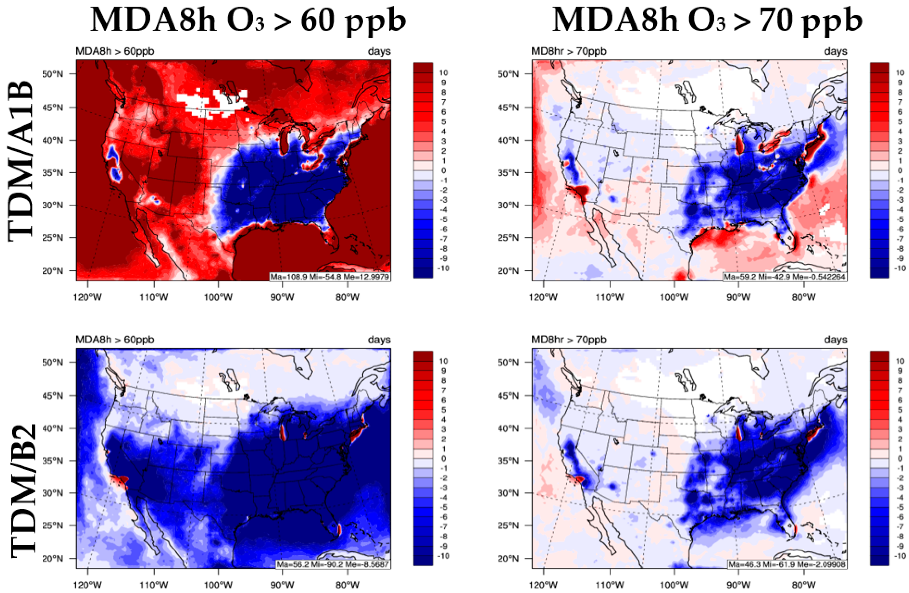
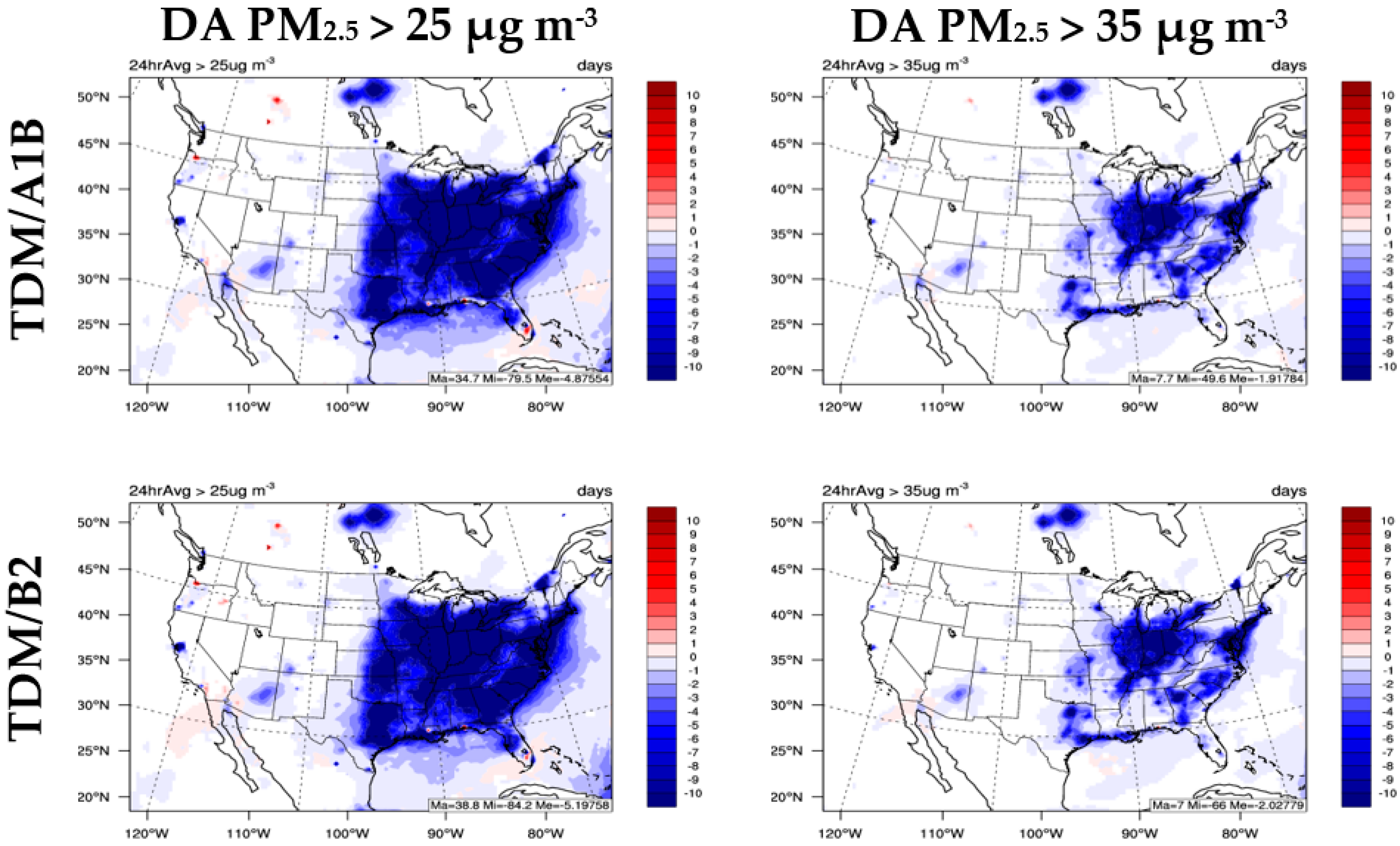
4.3. Impacts on Air Quality Exceedance Days

Figure 5 shows the spatial distribution of the average change in the number of O3 exceedance days with a threshold of 60 ppb and 70 ppb under TDM/A1B and TDM/B2 scenarios.
Ozone exceedance days are defined as the cumulative days with an MDA8 h greater than 70 ppb, which is the current O3 National Ambient Air Quality Standard (NAAQS), and for an MDA8 h O3 greater than 60 ppb, which reflects a possible lowering of the NAAQS in the near future (i.e., potential future national standards) [59]. The number of exceedance days of MDA8 h O3 > 70 ppb is significantly reduced but some areas remain in non-attainment, i.e., parts of California, Miami, Ohio River, the Great Lakes, and New York. The number of days of MDA8 h O3 > 60 ppb will increase over the U.S., except for the eastern U.S. and in some parts of California (Figure 5). While the overall MDA8 h O3 increases widely for the TDM/A1B scenario (Figure 3), the results here suggest that daytime O3 exceedances in the future may be reduced (i.e., a flattening of the diurnal O3 curve) in the eastern U.S., even in the advent of more stringent air quality regulations and lowering of the NAAQS for ozone (i.e., MDA8 h O3 > 60 ppb). Under more stringent regulations in the western U.S., however, more daytime O3 exceedances are projected under the future TDM/A1B scenario. Under the relatively more controlled TDM/B2 emission scenario, the daytime O3 exceedances in the future are reduced across the entire U.S. (Figure 5), except for some coastal/Great Lake regions, and in Los Angeles, CA, which may experience photochemical O3 regime shifts with such profound decreases in NOx emissions (i.e., potential shifts from VOC- to NOx-limited conditions in urban areas).
Figure 6 shows the spatial distribution of average change in the number of PM2.5 exceedance days for the TDM/A1B and TDM/B2 scenarios.
PM2.5 exceedance days are defined as the cumulative number of days with an average 24-h PM2.5 concentration greater than 35 µg m−3, which is the current PM2.5 NAAQS, and for average 24-h PM2.5 concentration greater than 25 µg m−3, which is the current World Health Organization (WHO) 24-h PM2.5 standard. Given the large reductions in PM2.5 concentrations for both TDM/A1B and TDM/B2 described previously (see Section 4.2 and Figure 4), the future number of PM2.5 exceedance days is significantly reduced over the U.S. under both the NAAQS and WHO 24-h regulatory standards. These results indicate that O3 and PM2.5 may be better controlled by reducing emissions of their precursors and GHGs with greater benefits under TDM/B2 than the TDM/A1B scenario.

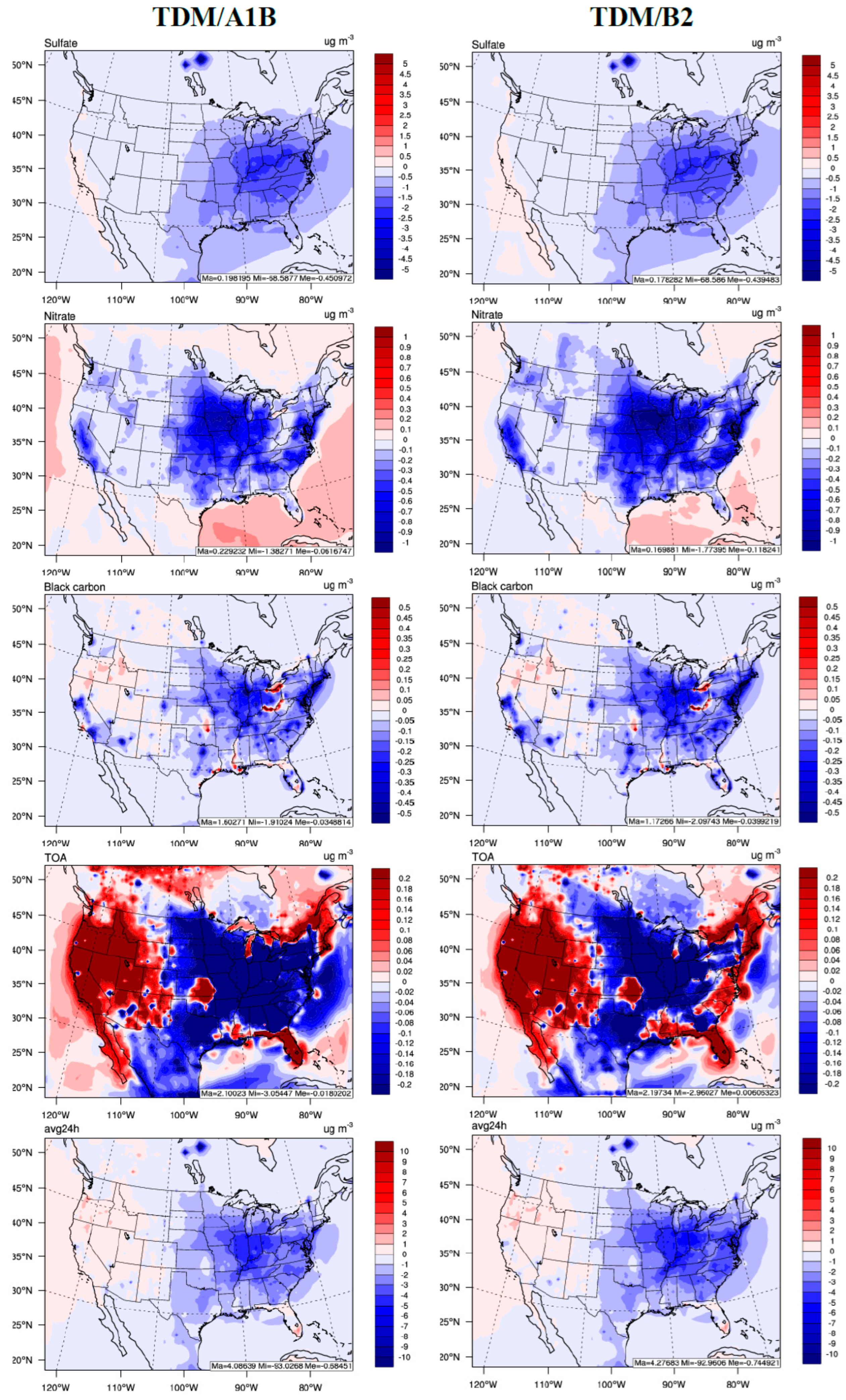
4.4. Impacts on Cloud-Aerosol Variables

The cloud condensation nuclei at supersaturation 0.5% (CCN5) and cloud droplet number concentration (CDNC) decrease over almost the whole domain for both the TDM/A1B and TDM/B2 scenarios (Figure 7). This is due to similar decreases in PM2.5 concentration spatial distributions, again most prolific over the eastern U.S. (see Section 4.2 and Figure 4). This is to be expected, as CCN is influenced by components of PM2.5 even though large uncertainties exist [60,61]. While not shown, the decreases in near-surface PM2.5 concentrations are in good agreement with the decreases in the total 3D column aerosol abundance (i.e., aerosol optical depth). The macroscopic cloud properties such as cloud fraction (CF) and cloud water path (CWP) decrease over most parts of the land area but increase over the ocean and over a portion of the southeastern U.S. The macroscopic CF and CWP are intrinsically linked to both the larger scale climate variable changes discussed in Section 4.1 (Figure 2 and Figure S4), but are also impacted by the microscopic cloud properties such as CCN5 and CDNC (Figure 7). Ultimately, the spatial distributions of CWP changes are inherently similar to those in PRECIP (Figure 2), which are driven by the relatively larger increases in moisture (Q2; Figure S4) over and transported from the ocean in both TDM/A1B (larger in magnitude) and TDM/B2 scenarios. We note that there are increases in CWP despite decreases in CDNC in the east-southeast U.S., which suggests the presence of more water vapor for available aerosols (and CCN5), thus driving the growth of larger cloud droplets and enhanced precipitation in the future for these regions.
The cloud optical thicknesses (COT) and shortwave cloud forcing (SWCF) generally have moderate to weak decreases over the whole domain except for the coastal and oceanic regions of the domain, which have larger increases for both TDM/A1B and TDM/B2 (Figure 7). The projected increases in COT, CWP, and SWCF indicate higher cloud amounts over the ocean in the eastern part of the domain, which results in a decrease in SWDOWN. In contrast, the projected decreases in COT, CWP, and SWCF over land indicate decreases in cloud amounts, which results in an increase in SWDOWN over land (Figure 2).
We note that the decrease in CCN5 for the TDM/B2 scenario, however, is slightly smaller on a domain-wide average than the TDM/A1B scenario, even though there are relatively larger decreases in PM2.5 concentrations for the TDM/B2 scenario (Figure 4). This is a consequence of smaller increases in Q2 and less available water vapor for CCN5 activation in TDM/B2 (Figure S4). The CDNC decreases are slightly larger due to larger decreases in PM2.5 for TDM/B2.

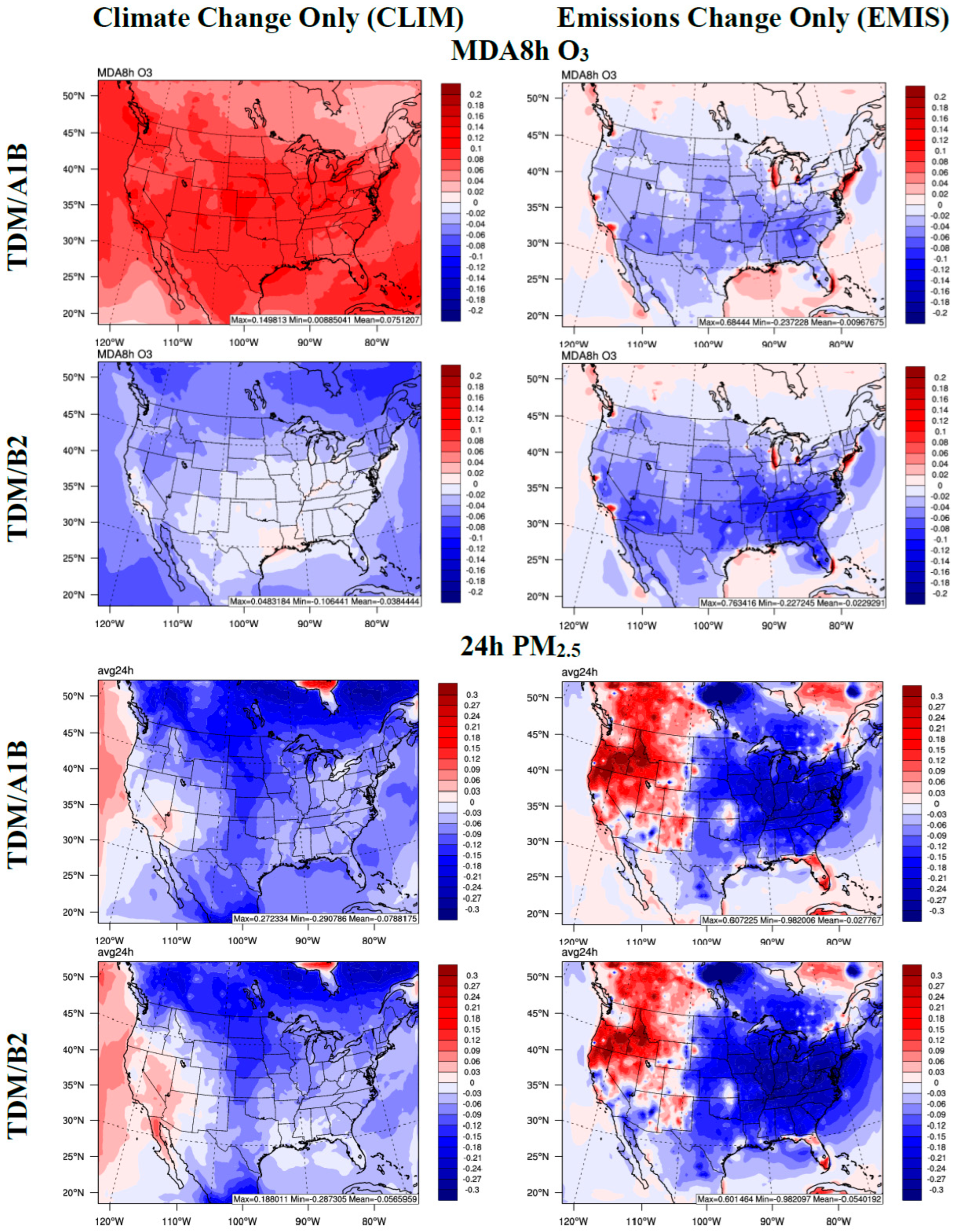
5. Impacts of Climate vs. Emission Changes on Future Air Quality

Both emission and climate changes each have a relative impact on future air quality. The impacts of climate changes only can also be derived based on CLIM_EMIS_A1B–EMIS_A1B, and CLIM_EMIS_B2-EMIS_B2 (CLIM_A1B and CLIM_B2, respectively; see Section 2, Table 1). We can thus study the relative importance of impacts from climate vs. emission changes on MDA8 h O3 and 24-h PM2.5 between the current and future decades (Figure 8), as compared with their combined changes (Figure 3 and Figure 4).
Figure 8 demonstrates that the widespread increases in future MDA8 h O3 concentrations in the TDM/A1B scenario (Figure 3) are driven by climate changes that consist of higher T2 (Figure 2) and CH4 concentrations, as well as the associated increases in biogenic VOC emissions (not shown). The impacts of SRES A1B climate change signal clearly dominate the anthropogenic TDM emissions change signal for MDA8 h O3. For the TDM/B2 scenario, however, the widespread decreases in MDA8 h O3 are dominated by the decreases in anthropogenic TDM emissions compared with the weaker climate signal for the B2 scenario. There is also some contribution to the future MDA8 h O3 decreases in the northwest U.S. from the B2 climate signal. We also note that in densely populated areas (i.e., the major U.S. cities), the increases in MDA8 h O3 are driven (and exacerbate the climate signal) by larger anthropogenic NOx emission reductions compared with VOC emission reductions in the VOC-limited O3 chemistry regions in both the TDM/A1B and TDM/B2 scenarios.
For the total 24-h PM2.5 changes in both the TDM/A1B and TDM/B2 scenarios, the widespread decreases in the eastern U.S. and weaker increases in the west-northwest (Figure 4) are clearly dominated by the anthropogenic TDM emissions signal (Figure 8). There are also smaller contributions from the A1B and B2 climate signals to the decreases in PM2.5 over the central/northern U.S. and increases in the west-southwest U.S. Furthermore, the anthropogenic TDM (both A1B and B2) emissions signals dominate the future PM2.5 increases in Florida. Overall, the large PM2.5 decreases (0–30%) in the eastern and central U.S. are due to decreases in the primary anthropogenic emissions of PM species and gaseous precursors, as well as decreases in the secondary formation of inorganic aerosols. There is a secondary effect of the climate signal with increased precipitation and wet deposition on reducing the future PM2.5.

6. Summary

In this work, we examine the impacts of both projected climate change and technology-driven emission changes on future meteorology, aerosol-clouds, and air quality under two IPCC SRES scenarios, which are modified with explicitly defined technology changes (i.e., TDM/A1B and TDM/B2) using the WRF/Chem model. The baseline simulations for 2001–2010 (representing the current climate and air quality) have been conducted and are well-evaluated [29]. Here, we employ WRF/Chem sensitivity simulations that use projected emissions from a novel TDM under both current and future climate conditions for 2046–2055 [25,26]. This simulation design allows for investigation of climate-only, emissions-only, and combined climate and emission impacts on meteorology, aerosol-clouds, and air quality changes.
The projected emissions showed widespread reductions in most gas and aerosol species under both TDM/A1B and TDM/B2 scenarios over the contiguous U.S. There is a widespread increase in MDA8 h O3 (domain-wide avg. ~ +2.6 ppb) in the TDM/A1B scenario due to enhanced CH4 concentrations and subsequent higher T2, increased biogenic VOC emissions, and larger NOx emission reduction than VOC emission reduction over VOC-limited O3 chemistry regions. The large increase in MDA8 h O3 between 10–22 ppb is found near and within major cities mainly in the northeastern U.S. and California. Overall, the impacts of climate change signal (i.e., “climate penalty”) dominate the impact of the anthropogenic TDM emissions decrease on the future overall increases of MDA8 h O3 for TDM/A1B. Despite the overall increases in MDA8 h O3 for TDM/A1B, the number of exceedance days (MDA8 h O3 > 70 and > 60 ppb) is reduced (avg. ~ −0.5 days), but some areas remain in non-attainment due to strong O3 increases (e.g., most of the western U.S., parts of Florida, Ohio River, the Great Lakes, and regions in the northeast U.S.). Thus, in the face of climate change, there is a clear indication of a strong impact of projected TDM/A1B emission changes on future air quality that can act to mitigate the climate signal in some regions (i.e., widespread regional/rural areas), while exacerbating it in others (i.e., localized urban/city areas). For the TDM/B2 scenario, there is a combined effect of climate and emission changes on domain-wide reductions in MDA8 h O3, which leads to widespread and significant reductions in the number of exceedance days in the future.
The daily 24-h average (DA24 h) PM2.5 levels are projected to similarly decrease (~0–30%) for both the TDM/A1B and TDM/B2 scenarios, most prolifically in the central and east U.S. and in parts of Canada and Mexico. This is due to synergetic effects of both the climate signal and TDM emission changes; however, the PM2.5 changes are dominated by the impacts from reduced anthropogenic primary aerosol and precursor gas emissions (for both TDM/A1B and TDM/B2), with a secondary effect of climate change on reducing PM2.5 in parts of the central and northern U.S. Consequently, the number of exceedance days (i.e., DA24 h PM2.5 > 35 µg m−3 or 25 µg m−3) is significantly reduced over the eastern U.S. under both TDM/A1B and B2 scenarios. We note that climate change does tend to increase the PM2.5 (climate penalty of ~ <10%) over parts of the west-southwest U.S. for both TDM A1B and TDM B2 scenarios.

7. Discussion

While our work agrees in part with the general spatial patterns and direction of air quality changes due to climate and emission changes from previous “big-picture”, top-down SRES and RCP scenario studies (see Section 1 for details), we expand upon such studies using a more explicit and detailed representation of the future anthropogenic emissions via the TDM approach in regional WRF/Chem. The TDM approach is a hybridization of an engineering (“bottom-up”) and economic (“top-down”) model, and thus we contend that it can more explicitly represent the projected anthropogenic emission inventories compared with previous studies, which allows us to better quantify the resulting U.S. state-level changes in air quality due to emissions only, climate change only, and their combined effects through our sensitivity simulations.
The detailed state-level TDM approach shows some pronounced differences in near-surface O3 concentrations compared with recent RCP-based studies. For example, our TDM/A1B results shows relatively more widespread spatial increases in O3 compared with a recent RCP 8.5 scenario study; however, the time periods and averaging compared differ (yearly at 2050 for TDM and seasonal at 2030 for RCP) [20]. We note that in this comparison, however, both studies agree in that in more extreme projection families (i.e., SRES/TDM A1B and RCP8.5), the combined future climate, background GHGs, and emission changes can lead to predominantly worsening air quality conditions and higher O3 in parts of the U.S. Our work also partly agrees with another RCP8.5 study in that a future warmer climate drives increases in O3; however, the inclusion of our explicit TDM/A1B emission changes do not as significantly counteract these increases enough to lead to overall O3 decreases in the RCP study [18]. Furthermore, our projected increase in MDA8 O3 is similar but on the lower end compared with the range of other studies on MDA8 O3 changes in the U.S. (3–5 ppb) that have used similar projection approaches [7]. Other SRES-only projection studies show potentially larger offsets to the climate-induced O3 increases due to larger anthropogenic emission reductions over the U.S. in their studies [10,11]; however, these studies used relatively simpler SRES-only emissions projection factors and less granular emission changes compared with the explicit TDM methodology at the U.S. state-level employed here.
It is difficult to find similar studies that have the same domain coverage, projection period, and averaging intervals, which leads to difficulty in making true “apples-to-apples” comparisons across different projection methodologies. Clearly, in our work, the inclusion of explicit TDM emission projections and increasing background GHGs leads to larger potential increases in O3 by 2050 in some U.S. regions compared with other previous studies. For PM2.5, the future air quality features greater reduction in PM2.5 by RCP 8.5/4.5 studies [23] than our TDM A1B/B2 work here, which is due to the inclusion of more explicit changes in precursors and primary emissions in the TDM approach. Our work does corroborate other studies that have shown future PM2.5 decreases in the southeast U.S. (annual average of ~1.0 µg m−3) [7]; however, we present larger magnitude decreases using the DA24 h analysis pertinent to shorter term exposure effects.
The results from this work add another possible future scenario (i.e., “SRES/TDM”) and show important differences in the changes of near-surface O3 and PM2.5 across the U.S. compared with the SRES-only and RCP scenarios. Thus, the results here are useful in further supporting the policy and regulatory analysis and assessment of the impacts of future control and changes in emissions on U.S. air quality in the face of imminent climate and emission changes. Ultimately, an ensemble of the different scenarios (SRES/TDM, SRES-only, and RCP) may be the best recommendation to evaluate potential future air quality changes in the U.S.

Supplementary Materials

The following supporting information can be downloaded at: https://www.mdpi.com/article/10.3390/atmos14020225/s1, Figure S1: Spatial distributions of relative (%) changes of CO, SO2, NOx, and VOC emissions between annual average of future (2046–2055) and present (2005) conditions under the TDM/A1B (top) and TDM/B2 (bottom) scenarios; Figure S2: Spatial distributions of absolute (top panel) relative (lower panel) changes of NH3, EC, SO42−, and PM2.5 emissions between annual average of future (2046–2055) and present (2005) conditions under the TDM/A1B scenario; Figure S3: Same as in Figure S2, but for the TDM/B2 scenario; Figure S4: Absolute changes of annual average 2-m water vapor mixing ratio (Q2), 10-m wind speed (WS10), and outgoing longwave radiation at the top of the atmosphere (OLR) between future and current decade for TDM/A1B (left) and TDM/B2 (right); Figure S5: Absolute changes of annual average of gaseous ammonia (NH3), ammonium (NH4+), primary organic aerosol (POA), and total secondary organic aerosol (TSOA) between the future and current decade for TDM/A1B and TDM/B2.

Author Contributions

Conceptualization, Y.Z.; methodology, C.J., Y.Z., K.W. and P.C.C.; software, K.W. and Y.Z.; validation, K.W. and Y.Z.; formal analysis, C.J., K.W. and P.C.C.; investigation, C.J., K.W. and P.C.C.; resources, Y.Z.; data curation, C.J., Y.Z., K.W. and P.C.C.; writing—original draft preparation, C.J.; writing—review and editing, Y.Z., K.W. and P.C.C.; visualization, C.J., K.W. and P.C.C.; supervision, Y.Z.; project administration, Y.Z.; funding acquisition, Y.Z. All authors have read and agreed to the published version of the manuscript.

Funding

This work was developed with support at North Carolina State University under the National Science Foundation EaSM program (AGS-1049200) and at North Carolina State University and Northeastern University under Assistance Agreement No. RD835871 awarded by the U.S. Environmental Protection Agency to Yale University. Extreme Science and Engineering Discovery Environment (XSEDE) digital service by the Texas Advanced Computing Center (TACC) (http://www.tacc.utexas.edu, accessed on 12 January 2023) was supported by National Science Foundation grant number ACI-1053575.

Institutional Review Board Statement

Not applicable.

Informed Consent Statement

Not applicable.

Data Availability Statement

The data used to generate results presented in this paper will be available free of charge upon request, please contact Yang Zhang at [email protected].

Acknowledgments

The projected emission changes under the TDM scenarios were generated by Fang Yan, Zifeng Lu, and David Streets under the USDA EaSM program (2012-67003-30192) at the University of Chicago/Argonne National Laboratory, Argonne, IL. High performance computing support from Yellowstone (ark:/85065/d7wd3xhc) and Cheyenne (doi:10.5065/D6RX99HX) provided by NCAR’s Computational and Information Systems Laboratory, sponsored by the National Science Foundation; and from Stampede and Stampede 2, provided as an Extreme Science and Engineering Discovery Environment (XSEDE) digital service by the Texas Advanced Computing Center (TACC) (http://www.tacc.utexas.edu, accessed on 12 January 2023).

Conflicts of Interest

The authors declare no conflict of interest.

Abbreviations

AER/AFWAAtmospheric and Environmental Research Inc. and Air Force Weather Agency
AQCHEM AQchemistry module based on CMAQ v4.7
BASE_EVALBase Evaluation model simulation in this work
BASE_TDMBase TDM reference model simulation in this work
BCBlack Carbon
BCONsBoundary Conditions
BVOCsBiogenic Volatile Organic Compounds
CB05Carbon Bond Mechanism 2005
CCNCloud Condensation Nuclei
CCN5Cloud Condensation Nuclei at Supersaturation 0.5%
CDNCCloud Droplet Number Concentration
CESM/CAMCommunity Earth System Model/Community Atmosphere Model
CFCloud Fraction
CLMCommunity Land Model
CLIM_EMIS_A1BFuture A1B climate + TDM/A1B scenario emissions model simulation in this work
CLIM_EMIS_B2Future B2 climate + TDM/B2 scenario emissions model simulation in this work
CONUSContiguous United States
COTCloud Optical Thickness
CWPCloud Water Path
DA24hDaily Average 24-h
EMIS_A1BFuture TDM/A1B scenario emissions model simulation in this work
EMIS_B2Future TDM/B2 scenario emissions model simulation in this work
EPAEnvironmental Protection Agency
FTUVFast Troposphere Ultraviolet Visible
GCMsGlobal Climate Models
GHGGreenhouse Gases
ICONsInitial Conditions
IPCCIntergovernmental Panel on Climate Change
LSMLand Surface Model
LWLongwave (Radiation)
MADE/VBSModal Aerosol Dynamics Model/Volatility Basis Set
MDA8Maximum Daily Average 8-h
MEGANModel of Emissions of Gases and Aerosols from Nature
MSKFMulti-Scale Kain Fritsch
NAAQSNational Ambient Air Quality Standard
NoahNational Center for Environmental Prediction, Oregon State University, Air Force and Hydrologic Research Lab
NCEP/FNLNational Centers for Environmental Prediction Final Analysis Dataset
NEINational Emissions Inventory
OAOrganic Aerosol
OLROutgoing Longwave Radiation at the Top of the Atmosphere
PBLPlanetary Boundary Layer
PBLHPlanetary Boundary Layer Height
PMParticulate Matter
POAPrimary Organic Aerosol
PRECIPPrecipitation (Total)
Q22-m Water Vapor Mixing Ratio
RCPRepresentative Concentration Pathways
RRTMGRapid Radiative Transfer Model for GCMs
SOASecondary Organic Aerosol
SPEW-TrendSpeciated Pollutant Emission Wizard-Trend
SRESSpecial Report on Emissions Scenarios
SWShortwave (Radiation)
SWCFShortwave Cloud Forcing
SWDOWNDownward Shortwave Radiation
T22-m Temperature
TNMVOCsTotal Non-Methane Volatile Organic Compounds
TDMTechnology Driver Model
TSOATotal Secondary Organic Aerosol
VOCsVolatile Organic Compounds
WHOWorld Health Organization
WRF/ChemWeather Research and Forecasting model coupled with Chemistry
WS1010-m Wind Speeds
YSUYonsei University

References

  1. World Meteorological Organization (WMO); United Nations Environment Programme; Intergovernmental Panel on Climate Change. Emissions Scenarios; IPCC Special Report; IPCC: Geneva, Switzerland, 2000; ISBN 92-9169-113-5. [Google Scholar]
  2. Moss, R.H.; Edmonds, J.A.; Hibbard, K.A.; Manning, M.R.; Rose, S.K.; Van Vuuren, D.P.; Carter, T.R.; Emori, S.; Kainuma, M.; Kram, T. The next generation of scenarios for climate change research and assessment. Nature 2010, 463, 747–756. [Google Scholar] [CrossRef]
  3. Bell, M.L.; Goldberg, R.; Hogrefe, C.; Kinney, P.L.; Knowlton, K.; Lynn, B.; Rosenthal, J.; Rosenzweig, C.; Patz, J.A. Climate change, ambient ozone, and health in 50 US cities. Clim. Change 2007, 82, 61–76. [Google Scholar] [CrossRef]
  4. Katragkou, E.; Zanis, P.; Kioutsioukis, I.; Tegoulias, I.; Melas, D.; Krüger, B.C.; Coppola, E. Future climate change impacts on summer surface ozone from regional climate-air quality simulations over Europe. J. Geophys. Res. Atmos. 2011, 116, D22307. [Google Scholar] [CrossRef] [Green Version]
  5. Carvalho, A.; Monteiro, A.; Solman, S.; Miranda, A.; Borrego, C. Climate-driven changes in air quality over Europe by the end of the 21st century, with special reference to Portugal. Environ. Sci. Policy 2010, 13, 445–458. [Google Scholar] [CrossRef] [Green Version]
  6. Nolte, C.G.; Gilliland, A.B.; Hogrefe, C.; Mickley, L.J. Linking global to regional models to assess future climate impacts on surface ozone levels in the United States. J. Geophys. Res. Atmos. 2008, 113, D14307. [Google Scholar] [CrossRef] [Green Version]
  7. Lam, Y.F.; Fu, J.S.; Wu, S.; Mickley, L.J. Impacts of future climate change and effects of biogenic emissions on surface ozone and particulate matter concentrations in the United States. Atmos. Meas. Tech. 2011, 11, 4789–4806. [Google Scholar] [CrossRef] [Green Version]
  8. Avise, J.; Chen, J.; Lamb, B.; Wiedinmyer, C.; Guenther, A.; Salathé, E.; Mass, C. Attribution of projected changes in summertime US ozone and PM2.5 concentrations to global changes. Atmos. Meas. Tech. 2009, 9, 1111–1124. [Google Scholar] [CrossRef] [Green Version]
  9. Kelly, J.; Makar, P.A.; Plummer, D.A. Projections of mid-century summer air-quality for North America: Effects of changes in climate and precursor emissions. Atmos. Meas. Tech. 2012, 12, 5367–5390. [Google Scholar] [CrossRef] [Green Version]
  10. Tagaris, E.; Manomaiphiboon, K.; Liao, K.-J.; Leung, L.R.; Woo, J.-H.; He, S.; Amar, P.; Russell, A.G. Impacts of global climate change and emissions on regional ozone and fine particulate matter concentrations over the United States. J. Geophys. Res. Atmos. 2007, 112, D14312. [Google Scholar] [CrossRef]
  11. Tao, Z.; Williams, A.; Huang, H.-C.; Caughey, M.; Liang, X.-Z. Sensitivity of U.S. surface ozone to future emissions and climate changes. Geophys. Res. Lett. 2007, 34, L08811. [Google Scholar] [CrossRef]
  12. Penrod, A.; Zhang, Y.; Wang, K.; Wu, S.-Y.; Leung, L.R. Impacts of future climate and emission changes on U.S. air quality. Atmos. Environ. 2014, 89, 533–547. [Google Scholar] [CrossRef]
  13. Wang, J.; Kotamarthi, V.R. High-resolution dynamically downscaled projections of precipitation in the mid and late 21st century over North America. Earths Futur. 2015, 3, 268–288. [Google Scholar] [CrossRef]
  14. Gao, Y.; Fu, J.S.; Drake, J.B.; Liu, Y.; Lamarque, J.-F. Projected changes of extreme weather events in the eastern United States based on a high resolution climate modeling system. Environ. Res. Lett. 2012, 7, 044025. [Google Scholar] [CrossRef] [Green Version]
  15. Gao, Y.; Fu, J.S.; Drake, J.B.; Lamarque, J.-F.; Liu, Y. The impact of emission and climate change on ozone in the United States under representative concentration pathways (RCPs). Atmos. Meas. Tech. 2013, 13, 9607–9621. [Google Scholar] [CrossRef] [Green Version]
  16. Trail, M.; Tsimpidi, A.P.; Liu, P.; Tsigaridis, K.; Hu, Y.; Nenes, A.; Russell, A.G. Downscaling a global climate model to simulate climate change over the US and the implication on regional and urban air quality. Geosci. Model Dev. 2013, 6, 1429–1445. [Google Scholar] [CrossRef] [Green Version]
  17. Sun, J.; Fu, J.S.; Huang, K.; Gao, Y. Estimation of future PM2.5 and ozone-related mortality over the continental United States in a changing climate: An application of high-resolution dynamical downscaling technique. J. Air Waste Manag. Assoc. 2015, 65, 611–623. [Google Scholar] [CrossRef] [Green Version]
  18. Pfister, G.G.; Walters, S.; Lamarque, J.-F.; Fast, J.; Barth, M.C.; Wong, J.; Done, J.; Holland, G.; Bruyère, C.L. Projections of future summertime ozone over the U.S. J. Geophys. Res. Atmos. 2014, 119, 5559–5582. [Google Scholar] [CrossRef]
  19. Li, K.; Liao, H.; Zhu, J.; Moch, J.M. Implications of RCP emissions on future PM2.5 air quality and direct radiative forcing over China. J. Geophys. Res. Atmos. 2016, 121, 12985–13008. [Google Scholar] [CrossRef] [Green Version]
  20. Nolte, C.G.; Spero, T.L.; Bowden, J.H.; Mallard, M.S.; Dolwick, P.D. The potential effects of climate change on air quality across the conterminous US at 2030 under three Representative Concentration Pathways. Atmos. Chem. Phys. 2018, 18, 15471–15489. [Google Scholar] [CrossRef] [PubMed] [Green Version]
  21. Fenech, S.; Doherty, R.M.; O’Connor, F.M.; Heaviside, C.; Macintyre, H.L.; Vardoulakis, S.; Agnew, P.; Neal, L.S. Future air pollution related health burdens associated with RCP emission changes in the UK. Sci. Total Environ. 2021, 773, 145635. [Google Scholar] [CrossRef]
  22. Yahya, K.; Wang, K.; Campbell, P.; Chen, Y.; Glotfelty, T.; He, J.; Pirhalla, M.; Zhang, Y. Decadal application of WRF/Chem for regional air quality and climate modeling over the U.S. under the representative concentration pathways scenarios. Part 1: Model evaluation and impact of downscaling. Atmos. Environ. 2017, 152, 562–583. [Google Scholar] [CrossRef] [Green Version]
  23. Yahya, K.; Campbell, P.; Zhang, Y. Decadal application of WRF/chem for regional air quality and climate modeling over the U.S. under the representative concentration pathways scenarios. Part 2: Current vs. future simulations. Atmos. Environ. 2017, 152, 584–604. [Google Scholar] [CrossRef] [Green Version]
  24. Rogelj, J.; Meinshausen, M.; Knutti, R. Global warming under old and new scenarios using IPCC climate sensitivity range estimates. Nat. Clim. Chang. 2012, 2, 248–253. [Google Scholar] [CrossRef]
  25. Yan, F.; Winijkul, E.; Streets, D.G.; Lu, Z.; Bond, T.C.; Zhang, Y. Global emission projections for the transportation sector using dynamic technology modeling. Atmos. Meas. Tech. 2014, 14, 5709–5733. [Google Scholar] [CrossRef] [Green Version]
  26. Campbell, P.; Zhang, Y.; Yan, F.; Lu, Z.; Streets, D. Impacts of transportation sector emissions on future U.S. air quality in a changing climate. Part I: Projected emissions, simulation design, and model evaluation. Environ. Pollut. 2018, 238, 903–917. [Google Scholar] [CrossRef] [PubMed]
  27. Campbell, P.; Zhang, Y.; Yan, F.; Lu, Z.; Streets, D. Impacts of transportation sector emissions on future U.S. air quality in a changing climate. Part II: Air quality projections and the interplay between emissions and climate change. Environ. Pollut. 2018, 238, 918–930. [Google Scholar] [CrossRef]
  28. Grell, G.A.; Peckham, S.E.; Schmitz, R.; McKeen, S.A.; Frost, G.; Skamarock, W.C.; Eder, B. Fully coupled “online” chemistry within the WRF model. Atmos. Environ. 2005, 39, 6957–6975. [Google Scholar] [CrossRef]
  29. Wang, K.; Zhang, Y.; Yahya, K. Decadal application of WRF/Chem over the continental U.S.: Simulation design, sensitivity simulations, and climatological model evaluation. Atmos. Environ. 2021, 253, 118331. [Google Scholar] [CrossRef]
  30. Clough, S.; Shephard, M.; Mlawer, E.; Delamere, J.; Iacono, M.; Cady-Pereira, K.; Boukabara, S.; Brown, P. Atmos. radiative transfer modeling: A summary of the AER codes. J. Quant. Spectrosc. Radiat. Transf. 2005, 91, 233–244. [Google Scholar] [CrossRef]
  31. Iacono, M.J.; Delamere, J.S.; Mlawer, E.J.; Shephard, M.W.; Clough, S.A.; Collins, W.D. Radiative forcing by long-lived greenhouse gases: Calculations with the AER radiative transfer models. J. Geophys. Res. Atmos. 2008, 113, D13103. [Google Scholar] [CrossRef]
  32. Hong, S.-Y.; Noh, Y.; Dudhia, J. A New Vertical Diffusion Package with an Explicit Treatment of Entrainment Processes. Mon. Weather. Rev. 2006, 134, 2318–2341. [Google Scholar] [CrossRef] [Green Version]
  33. Hong, S.-Y. A new stable boundary-layer mixing scheme and its impact on the simulated East Asian summer monsoon. Quart. J. Roy. Meteorol. Soc. 2010, 136, 1481–1496. [Google Scholar] [CrossRef]
  34. Chen, F.; Dudhia, J. Coupling an advanced land surface hydrology model with the Penn State–NCAR MM5 Modeling sys-tem. Part I: Part I: Model Implementation and Sensitivity. Mon. Wea. Rev. 2001, 129, 569–585. [Google Scholar] [CrossRef]
  35. Ek, M.B.; Mitchell, K.E.; Lin, Y.; Rogers, E.; Grunmann, P.; Koren, V.; Gayno, G.; Tarpley, J.D. Implementation of Noah land surface model advances in the National Centers for Environmental Prediction operational mesoscale Eta model. J. Geophys. Res. Atmos. 2003, 108, 8851. [Google Scholar] [CrossRef]
  36. Morrison, H.; Thompson, G.; Tatarskii, V. Impact of Cloud Microphysics on the Development of Trailing Stratiform Precipitation in a Simulated Squall Line: Comparison of One and Two-Moment Schemes. Mon. Weather. Rev. 2009, 137, 991–1007. [Google Scholar] [CrossRef] [Green Version]
  37. Zheng, Y.; Alapaty, K.; Herwehe, J.A.; Del Genio, A.; Niyogi, D. Improving High-Resolution Weather Forecasts Using the Weather Research and Forecasting (WRF) Model with an Updated Kain–Fritsch Scheme. Mon. Weather Rev. 2016, 144, 833–860. [Google Scholar] [CrossRef]
  38. Yarwood, G.; Rao, S.; Yocke, M.; Whitten, G.Z. Final Report e Updates to the Carbon Bond Mechanism: CB05; Rep. RT-04-00675; Yocke and Co.: Novato, CA, USA, 2005; p. 246. [Google Scholar]
  39. Sarwar, G.; Bhave, P.V. Modeling the Effect of Chlorine Emissions on Ozone Levels over the Eastern United States. J. Appl. Meteorol. Clim. 2007, 46, 1009–1019. [Google Scholar] [CrossRef] [Green Version]
  40. Tie, X.; Madronich, S.; Walters, S.; Zhang, R.; Rasch, P.; Collins, W. Effect of clouds on photolysis and oxidants in the troposphere. J. Geophys. Res. 2003, 108, 4642. [Google Scholar] [CrossRef]
  41. Ackermann, I.J.; Hass, H.; Memmesheimer, M.; Ebel, A.; Binkowski, F.S.; Shankar, U. Modal aerosol dynamics model for Europe: Development and first applications. Atmos. Environ. 1998, 32, 2981–2999. [Google Scholar] [CrossRef]
  42. Ahmadov, R.; McKeen, S.A.; Robinson, A.; Bahreini, R.; Middlebrook, A.; de Gouw, J.; Meagher, J.F.; Hsie, E.-Y.; Edgerton, E.S.; Shaw, S.; et al. A volatility basis set model for summertime secondary organic aerosols over the eastern United States in 2006. J. Geophys. Res. 2012, 117, D06301. [Google Scholar] [CrossRef]
  43. Abdul-Razzak, H.; Ghan, S. A parameterization of aerosol activation: 2. Multiple aerosol types. J. Geophys. Res. 2000, 105, 6837–6844. [Google Scholar] [CrossRef]
  44. Glotfelty, T.; Zhang, Y. Impact of future climate policy scenarios on air quality and aerosol-cloud interactions using an advanced version of CESM/CAM5: Part II. Future trend analysis and impacts of projected anthropogenic emissions. Atmos. Environ. 2017, 152, 531–552. [Google Scholar] [CrossRef] [Green Version]
  45. Glotfelty, T.; He, J.; Zhang, Y. Improving organic aerosol treatments in CESM/CAM 5: Development, application, and evaluation. J. Adv. Model. Earth Syst. 2017, 9, 1506–1539. [Google Scholar] [CrossRef] [Green Version]
  46. U.S. Environmental Protection Agency. National Emissions Inventories. Available online: https://www.epa.gov/air-emissions-inventories (accessed on 18 November 2022).
  47. Guenther, A.; Karl, T.; Harley, P.; Wiedinmyer, C.; Palmer, P.I.; Geron, C. Estimates of global terrestrial isoprene emissions using MEGAN (Model of Emissions of Gases and Aerosols from Nature). Atmos. Chem. Phys. 2006, 6, 3181–3210. [Google Scholar] [CrossRef] [Green Version]
  48. Jones, S.; Creighton, G. AFWA Dust Emission Scheme for WRF/Chem-GOCART; WRF workshop: Boulder, CO, USA, 2011. [Google Scholar]
  49. LeGrand, S.L.; Polashenski, C.; Letcher, T.W.; Creighton, G.A.; Peckham, S.E.; Cetola, J.D. The AFWA dust emission scheme for the GOCART aerosol model in WRF-Chem v3.8.1. Geosci. Model Dev. 2019, 12, 131–166. [Google Scholar] [CrossRef] [Green Version]
  50. Gong, S.L.; Barrie, L.A.; Blanchet, J.-P. Modeling sea-salt aerosols in the atmosphere: 1. Model development. J. Geophys. Res. Atmos. 1997, 102, 3805–3818. [Google Scholar] [CrossRef] [Green Version]
  51. Wang, K.; Zhang, Y.; Yahya, K.; Wu, S.-Y.; Grell, G. Implementation and initial application of new chemistry-aerosol options in WRF/Chem for simulating secondary organic aerosols and aerosol indirect effects for regional air quality. Atmos. Environ. 2015, 115, 716–732. [Google Scholar] [CrossRef]
  52. He, J.; Zhang, Y. Improvement and further development in CESM/CAM5: Gas-phase chemistry and inorganic aerosol treatments. Atmos. Meas. Tech. 2014, 14, 9171–9200. [Google Scholar] [CrossRef] [Green Version]
  53. Xu, Z.; Yang, Z.-L. An Improved Dynamical Downscaling Method with GCM Bias Corrections and Its Validation with 30 Years of Climate Simulations. J. Clim. 2012, 25, 6271–6286. [Google Scholar] [CrossRef]
  54. Yan, F.; Winijkul, E.; Jung, S.; Bond, T.; Streets, D. Global emission projections of particulate matter (PM): I. Exhaust emissions from on-road vehicles. Atmos. Environ. 2011, 45, 4830–4844. [Google Scholar] [CrossRef]
  55. U.S. Department of Energy. Annual Energy Outlook 2013 with Projections to 2040. Available online: https://www.osti.gov/servlets/purl/1081575.DOE/EIA-0383(2013) (accessed on 18 November 2022).
  56. Nazarenko, L.; Schmidt, G.A.; Miller, R.L.; Tausnev, N.; Kelley, M.; Ruedy, R.; Russell, G.L.; Aleinov, I.; Bauer, M.; Bauer, S.; et al. Future climate change under RCP emission scenarios with GISS ModelE2. J. Adv. Model. Earth Syst. 2015, 7, 244–267. [Google Scholar] [CrossRef] [Green Version]
  57. Separovic, L.; Alexandru, A.; Laprise, R.; Martynov, A.; Sushama, L.; Winger, K.; Tete, K.; Valin, M. Present climate and climate change over North America as simulated by the fifth-generation Canadian regional climate model. Clim. Dyn. 2013, 41, 3167–3201. [Google Scholar] [CrossRef] [Green Version]
  58. Pfleiderer, P.; Nath, S.; Schleussner. Extreme Atlantic hurricane seasons made twice as likely by ocean warming. Weather Clim. Dynam. 2022, 4, 1–12. [Google Scholar] [CrossRef]
  59. U.S. EPA. Overview of EPA’S Updates to the Air Quality Standards for Ground-Level Ozone, the National Ambient Air Quality Standards. Available online: https://www.epa.gov/sites/default/files/2015-10/documents/overview_of_2015_rule.pdf (accessed on 18 November 2022).
  60. Yu, S. The role of organic acids (formic, acetic, pyruvic, and oxalic) in the formation of cloud condensation nuclei (CCN): A review. Atmos. Res. 2000, 53, 185–217. [Google Scholar] [CrossRef]
  61. Valin, L.C.; Russell, A.R.; Cohen, R.C. Chemical feedback effects on the spatial patterns of the NOx weekend effect: A sensitivity analysis. Atmos. Meas. Tech. 2014, 14, 1–9. [Google Scholar] [CrossRef]
Figure 1. Spatial distributions of absolute changes of CO, SO2, NOx, and VOC emissions between annual average of future (2046–2055) and present, baseline (2005) conditions under the TDM/A1B (top) and TDM/B2 (bottom) scenarios.
Atmosphere 14 00225 g001
Figure 2. Absolute changes of annual average temperature at 2-m (T2), shortwave downward radiation at the surface (SWDOWN), planetary boundary layer height (PBLH), and total precipitation (PRECIP) between the future and current decade for TDM/A1B (left) and TDM/B2 (right).
Atmosphere 14 00225 g002
Figure 3. Absolute changes of annual average carbon monoxide (CO), nitrogen dioxide (NO2), total non-methane volatile organic compounds (TNMVOCs), sulfur dioxide (SO2), and daily maximum 8 h ozone (O3) between the future and current decade for TDM/A1B and TDM/B2.
Atmosphere 14 00225 g003
Figure 4. Absolute changes of annual average sulfate (SO42−), nitrate (NO3), black carbon (BC), total organic aerosol (TOA), and daily average PM2.5 (DA24 h) between the future and current decade for TDM/A1B and TDM/B2.
Atmosphere 14 00225 g004
Figure 5. Absolute changes of average number of exceedance days of MDA8 h O3 with a threshold of 60 ppb and 70 ppb between the future and current decade for TDM/A1B and TDM/B2.
Atmosphere 14 00225 g005
Figure 6. Absolute changes of average number of exceedance days of 24-h daily averaged (DA) PM2.5 against a threshold of 25 µg m−3 and 35 µg m−3 between the future and current decade for TDM/A1B and TDM/B2.
Atmosphere 14 00225 g006
Figure 7. Absolute changes of annual average cloud condensation nuclei at supersaturation 0.5% (CCN5), cloud droplet number concentration (CDNC), cloud fraction (CF), cloud optical thickness (COT), cloud water path (CWP), and shortwave cloud forcing (SWCF) between the future and current decade for TDM/A1B and TDM/B2.
Atmosphere 14 00225 g007
Figure 8. The changes in MDA8 h O3 (top four panels) and 24-h PM2.5 (bottom four panels) due to climate changes only (left column; CLIM) and emission changes only (right column; EMIS). See Table 1 for descriptions of the model sensitivities and derived impact assessments.
Atmosphere 14 00225 g008
Table 1. Baseline simulations, additional TDM simulations, and derived results for impact assessments in this work.
Simulation
Index
Emission ScenarioAnthro.
Emissions
Climate
Conditions
Purpose or Impact AssessmentReference
BASE_EVALNoneNEI 2002, 2005, and 20082001–2010Model performance evaluation[29]
BASE_TDMNoneTDM Base
2005
2001–2010Benchmark for other scenariosThis work
EMIS_A1BTDM/ A1BTDM/A1B
2046–2055
2001–2010TDM/A1B
Emissions Only
(compared to BASE_TDM)
This work
EMIS_B2TDM/B2TDM/B2
2046–2055
2001–2010TDM/B2
Emissions Only
(compared to BASE_TDM)
This work
CLIM_A1B *TDM/A1BTDM/A1B
2046–2055
2046–2055A1B
Climate Only (compared to EMIS_A1B)
This work
CLIM_B2 *TDM/B2TDM/B2
2046–2055
2046–2055B2
Climate Only (compared to EMIS_B2)
This work
CLIM_EMIS_A1BA1BTDM/A1B
2046–2055
2046–2055A1B Climate + TDM/A1B Emissions (compared to BASE_TDM)This work
CLIM_EMIS_B2B2TDM/B2
2046–2055
2046–2055B2 Climate + TDM/B2 Emissions (compared to BASE_TDM)This work
* CLIM_A1B is derived using CLIM_EMIS_A1B and EMIS_A1B; and CLIM_B2 is derived using CLIM_EMIS_B2 and EMIS_B2.
Table 2. WRF/Chem model configuration, physics and chemistry options, and major inputs used in this study.
Model AttributesConfiguration
ModelOnline-coupled WRF/Chem v3.7
Domain and resolutions36 km × 36 km, 148 × 112 horizontal resolution over the continental US with 34 layers vertically from surface to 100 hpa
Simulation periodCurrent decade 2001–2010 and future decade 2046–2055
Physics and Chemistry options [Reference(s)]
RadiationRapid and accurate Radiative Transfer Model for GCM (RRTMG) SW and LW [30,31]
Boundary layerYonsei University (YSU) [32,33]
Land surface modelNational Center for Environmental Prediction, Oregon State University, Air Force and Hydrologic Research Lab (Noah) [34,35]
MicrophysicsMorrison double moment scheme [36]
Cumulus parameterizationMulti-Scale Kain Fritsch (MSKF) [37]
Gas-phase chemistryModified CB05 with updated chlorine chemistry [38,39]
PhotolysisFast Troposphere Ultraviolet Visible (FTUV) [40]
Aqueous-phase chemistryAQ chemistry module (AQCHEM) based on CMAQv4.7 implementation for both resolved and convective clouds
Aerosol moduleModal Aerosol Dynamics Model/Volatility Basis Set(MADE/VBS) [41,42]
Aerosol activationAbdul-Razzak and Ghan [43]
Inputs [Reference(s)]
Chemical and meteorological ICs/BCsDownscaled from the Modified Community Earth System Model/Community Atmosphere model (CESM/CAM5) v1.2.2; Meteorology ICONs/BCONs bias-corrected with NCEP/FNL. [44,45]
Anthropogenic emissionsU.S. EPA National Emissions Inventory 2002, 2005, 2008 for the current decade; TDM-projected growth factor under the IPCC/A1B and B2 scenarios based on 2005 emission. [25] and [46]
Biogenic emissionsModel of Emissions of Gases and Aerosols from Nature version 2 (MEGAN v2) [47]
Dust emissionsAtmospheric and Environmental Research Inc. and Air Force Weather Agency (AER/AFWA) [48,49]
Sea-salt emissionsGong et al. parameterization [50]
Disclaimer/Publisher’s Note: The statements, opinions and data contained in all publications are solely those of the individual author(s) and contributor(s) and not of MDPI and/or the editor(s). MDPI and/or the editor(s) disclaim responsibility for any injury to people or property resulting from any ideas, methods, instructions or products referred to in the content.

