
Evaluation of an Ocean Reanalysis System in the Indian and Pacific Oceans
Institute of Atmospheric Physics, Chinese Academy of Sciences, Beijing 100029, China
*
Author to whom correspondence should be addressed.
Atmosphere 2023, 14(2), 220; https://doi.org/10.3390/atmos14020220
Submission received: 10 December 2022
/
Revised: 13 January 2023
/
Accepted: 19 January 2023
/
Published: 20 January 2023
(This article belongs to the Special Issue Climate Change on Ocean Dynamics)
Abstract
:This paper describes an ocean reanalysis system in the Indian and Pacific oceans (IPORA) and evaluates its quality in detail. The assimilation schemes based on ensemble optimal interpolation are employed in the hybrid coordinate ocean model to conduct a long-time reanalysis experiment during the period of 1993–2020. Different metrics including comparisons with satellite sea surface temperature, altimetry data, observed currents, as well as other reanalyses such as ECCO and SODA are used to validate the performance of IPORA. Compared with the control experiment without assimilation, IPORA greatly reduces the errors of temperature, salinity, sea level anomaly, and current fields, and improves the interannual variability. In contrast to ECCO and SODA products, IPORA captures the strong signals of SLA variability and reproduces the linear trend of SLA very well. Meanwhile, IPORA also shows a good consistence with observed currents, as indicated by an improved correlation and a reduced error.
1. Introduction
The data assimilation combining numerical models with observations to obtain the statistically best estimate has been widely recognised as a powerful tool in oceanographic and meteorological research. Reanalyses are reconstructions of a long-term historical dataset for the states via data assimilation methods. Ocean reanalyses originate from the efforts of meteorologists in the 1990s to reconstruct the time evolution of the global atmosphere state [1]. One application of these atmosphere reanalyses is to provide surface forcing fields which the oceanographers use to drive ocean models [2,3,4,5]. Similar to atmosphere reanalyses, ocean reanalyses, which combine different types of observations with ocean models, have the potential to provide dynamically consistent and accurate estimates of the ocean states [6].
Ocean reanalyses at the global and regional scales have already become available and been an established activity in some research and operational centres with enhancements of ocean observing systems such as satellite data, Argo floats, and other observing platforms. The SODA (simple ocean data assimilation) ocean reanalysis was produced by the optimal interpolation method in the global oceans [2,3,7]. The ocean reanalysis systems developed at the European Centre for Medium-Range Weather Forecasts (ECMWF) used different assimilation methods including optimal interpolation and variational assimilation NEMOVAR in different versions [8,9]. The ECCO (estimating the circulation and climate of the ocean) reanalysis was generated by the four-dimensional variational (4DVAR) method [10,11]. The MOVE (Multivariate Ocean Variational Estimation) reanalyses were based on the three-dimensional variational (3DVAR) scheme [12,13,14,15]. The TOPAZ4 reanalysis was based on the ensemble Kalman filter in the North Atlantic and the Arctic [16,17]. The CORA (China Ocean Reanalysis) used a 3DVAR-based multi-scale scheme in the China coastal seas and global oceans, respectively [18,19]. The FORA-WNP30 reanalysis focused on the western North Pacific [20]. Dwivedi et al. [21] evaluated a 4DVAR assimilation system in the northern Indian Ocean. Additionally, some intercomparisons of established reanalysis products were made in the tropical Indian Ocean [22]. However, some ocean reanalyses do not use all observations due to the limitations imposed by the assimilation techniques and observation data types [7,14,15,23,24,25,26,27,28]. The advancement of the assimilation methods and the enhancement of observing networks promote the generation of reanalyses that allow for the use of a variety of observations [29,30,31,32]. Therefore, the improvements in the model resolution, physics, atmospheric forcings, observation data types, and assimilation methods will lead to the successive generation of ocean reanalyses. This paper is to fully utilise a variety of available observations to produce an ocean reanalysis via the ensemble-optimal-interpolation-based schemes in the Indian and Pacific oceans.
The aim of this paper is to provide detailed description and validation for the ocean reanalysis system in the Indian and Pacific oceans. Configurations of the data assimilation scheme are described in Section 2. The reanalysis setup and evaluation through comparisons with observations, SODA, and ECCO are presented in Section 3. The conclusion and discussion are given in Section 4.
2. Ocean Data Assimilation System
The ocean data assimilation system used here consists of an ocean circulation model, the ensemble-based assimilation schemes, and a variety of observations. The details are described in this section.
2.1. Ocean Model
The ocean model used here is version 2.2 of the hybrid coordinate ocean model (HYCOM) developed at the University of Miami [33,34] and updated by the Nansen Environmental and Remote Sensing Center in Norway [16,35]. It has three vertical coordinates corresponding to different depths. The isopycnic coordinates are applied in the open and stratified ocean and smoothly transit to z coordinates in the weakly stratified mixed layer to terrain-following sigma coordinates in shallow water regions, and back to z coordinates in very shallow water. The hybrid coordinates have a great advantage in good representation of ocean thermodynamic processes and ocean currents. The 28 hybrid z-isopycnal vertical layers are used in this paper. The top five layers remain z-level coordinate with a minimum thickness of 2 m. The model domain covers the Indian and Pacific oceans, spanning from 30° E to 70° W zonally and from 51° S to 61° N meridionally. The model has a horizontal resolution of about 1/3°. The K-profile parameterisation scheme [36] is used to compute the vertical mixing coefficient. A relaxation to climatological temperature and salinity with a restoring time scale of 30 days is applied at the sea surface and lateral boundary. The model is driven by the forcing fields including the 6-h air temperature, dew temperature, winds, mean sea level pressure, total cloud cover, and precipitation from the atmospheric reanalysis ERA-interim [37] at the surface.
The model is initialised from rest and climatological temperature and salinity fields used at the boundary. Then, a 10-year spin-up experiment that uses climatological atmospheric forcings from ERA-40 is carried out. The last day of the spin-up run provides the initial conditions for this reanalysis.
2.2. Observations
This reanalysis assimilates observations from satellite sea level anomaly (SLA), satellite sea surface temperature (SST), and in situ temperature (T) and salinity (S) profiles.
The SLA observations assimilated are sourced from the global gridded product with a horizontal resolution of 1/4° and a temporal resolution of 1 day delivered by the Sea Level TAC (Thematic Assembly Centre) of the Copernicus Marine Environment Monitoring Service (CMEMS) project. It is estimated by optimal interpolation, merging the L3 along-track measurement from all altimeter missions including Sentinel-3A, Jason-3, HY-2A, Saral/AltiKa, Cryosat-2, OSTM/Jason-2, Jason-1, Topex/Poseidon, Envisat, GFO, and ERS-1/2.
The SST observations assimilated come from the NOAA high-resolution daily analysis product OISST at a spatial resolution of 1/4° × 1/4° and a temporal resolution of 1 day with global coverage [38]. It was generated by combining the SST data from AVHRR (Advanced Very High Resolution Radiometer) infrared radiances and AMSR-E (Advanced Microwave Scanning Radiometer-EOS) microwave radiances which are available from June 2002 to October 2011 with in situ data from ships and buoys via the optimum interpolation method. Moreover, some improvements in the data sources, correction methods, and sea-ice-concentration to SST conversion methods were implemented for these analyses from April 2020 onwards [39,40].
All in situ temperature and salinity observations sourced from Argo, the Arctic Synoptic Basin-wide Oceanography (ASBO) project, the Global Temperature and Salinity Profile Programme (GTSPP), and the World Ocean Database 2018 (WOD18) are extracted from the ENSEMBLES EN4.2.2 dataset [41]. The Mechanical BathyThermograph (MBTs) and eXpendable BathyThermograph (XBT) data were corrected [42,43]. This dataset was collected, quality-checked, and released by the U.K. Met Office Hadley Centre.
These observations are pretreated before the assimilation. The super-observation method is applied in order to filter some noise or eliminate redundant information relative to the model. This method is widely employed in data assimilation [44]. For SST and SLA observations, a super-observation is generated by a simple weight average over all observations in every 2 × 2 model grid cell. For T and S profiles, a super-observation is a good profile selected from all profile observations falling in each 2 × 2 model grid bin since the horizontal average may cause some problems. According to the quality of the observations, the selection criteria are as follows: first Argo, then CTD, TAO, and, finally, XBT/MBT. These super-observations are used for the assimilation.
2.3. Assimilation Scheme
The ocean data assimilation schemes used in this paper are based on the ensemble optimal interpolation (EnOI) method [45]. The analysis fields are estimated by solving the following equations:
where represents the model state vector including temperature, salinity, layer thickness, baroclinic and barotropic current fields, and barotropic pressure. The superscripts a, b, and T denote analysis, background, and matrix transpose, respectively. H is the observation operator that interpolates from model grids to observation locations. P is the background error covariance matrix. L is a correlation function used to localise the background error covariance. The circle between L and P denotes a Schur product. R is the observation error covariance matrix. Since the observation errors are assumed to be uncorrelated in space and time, R is a diagonal matrix. is a scalar that can be used to tune the weights on the ensemble versus observations. Here it is taken as 0.4.
Estimates of the background error covariance matrix P are given by
where A is an ensemble anomaly from a long-term model integration with no data assimilation and n is the ensemble size (n = 120 here).
The assimilation schemes corresponding to different observations based on the EnOI method are employed. A different scheme is used to assimilate T/S profiles due to the isopycnic coordinate [46]. The layer thickness computed from temperature and salinity observations is assimilated to adjust the model layer thickness and current fields. Then, the temperature or salinity observations are assimilated to adjust the model temperature or salinity followed by diagnosing the salinity or temperature from the equation of the seawater state. A vertical localization technique, which confines the influence of SST observations to the mixed layer, is employed to assimilate SST [47]. The mean dynamic topography used in the reanalysis is the mean sea surface height calculated from the experiment with T/S assimilation, instead of the experiment without assimilation [48]. These schemes are combined to assimilate multi-source observations.
3. Results
This section describes settings and assessment of the reanalysis. To demonstrate the quality of the reanalysis dataset, we compare reanalysed fields with observations, with reanalysis products such as ECCO and SODA, as well as with a control experiment without assimilation. The independent observations such as observed current fields and withdrawn temperature and salinity profiles are used to further validate the performance of the reanalysis.
3.1. Reanalysis Settings
The reanalysis settings are summarised in Table 1. The reanalysis is generated by a data assimilation experiment in which temperature and salinity profiles, remotely sensed SST, and altimetry SLA observations are assimilated into HYCOM via EnOI at a 7-day assimilation frequency in the Indian and Pacific oceans during the period 1993–2020 (hereafter called IPORA). Moreover, the multi-year control experiment (CNTL hereafter) with no data assimilation is implemented to provide ensemble members for estimation of the background error covariance matrix and also to be used for validation of IPORA.
3.2. Temperature and Salinity
The SST data from OISST are used to evaluate the fit of IPORA to the observations. Meanwhile, some temperature and salinity profiles are withdrawn and not used in the IPORA. Therefore, they are regarded as independent observations to further validate the performance of IPORA. The root mean square error (RMSE) is used as a quality metric.
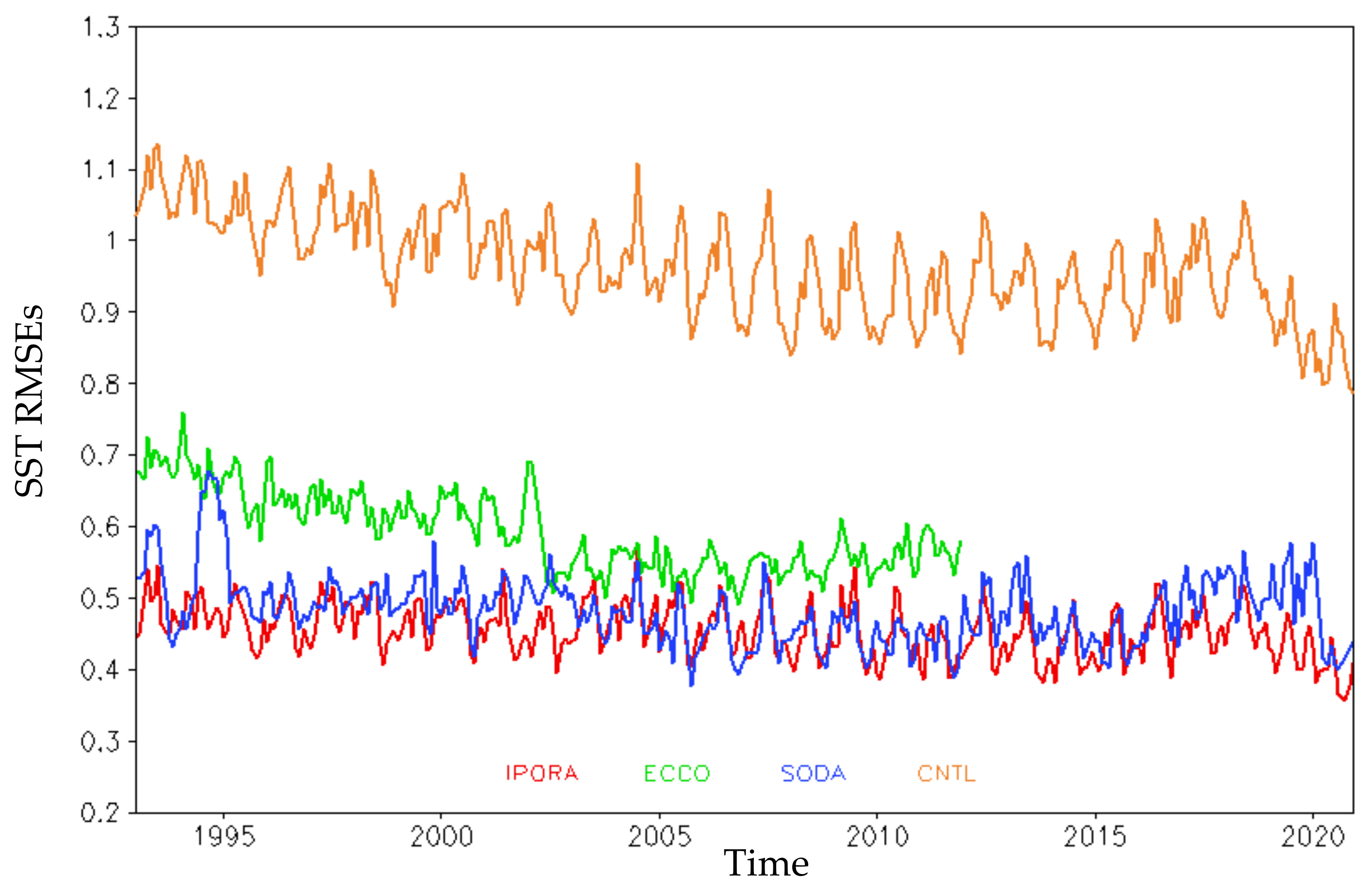
Figure 1 shows the time evolution of SST RMSEs in the model domain from all analyses. Note that the ECCO product is available only before 2012. It is version 4 release 2 of ECCO with a horizontal resolution of 0.5° [49,50]. The SODA product used here is the version 3.4.2 [7]. It has a uniform 0.5° × 0.5° horizontal grid on which the original 0.25° × 0.25° grid is regridded. The SST RMSEs of the control experiment without assimilation are approximately 0.95 °C during the period 1993–2020, and the RMSEs of the three reanalyses data are reduced to less than 0.7 °C. This result indicates that the fit to the observations may be improved greatly by the assimilation. The RMSEs of ECCO are larger than those of IPORA and SODA. IPORA slightly improves the fit compared with SODA. Additionally, the sudden reduction in RMSEs in 2020 may be associated with the improvements implemented in OISST due to the presence of biases. Figure 2 shows the spatial distribution of SST RMSEs against OISST over the period 1993–2020. The control experiment without assimilation demonstrates large RMSEs in regions with abundant eddies (e.g., the Kuroshio and Agulhas) and coastal regions. IPORA, ECCO, and SODA greatly improve the fit to observations in the Indian and Pacific oceans. Visually, IPORA has a good fit to the observations. The SST RMSEs from IPORA are reduced to less than 0.4 °C in most regions. The fit of SODA to the observations is also visibly improved but is not better than IPORA. ECCO presents larger RMSEs than both IPORA and SODA.
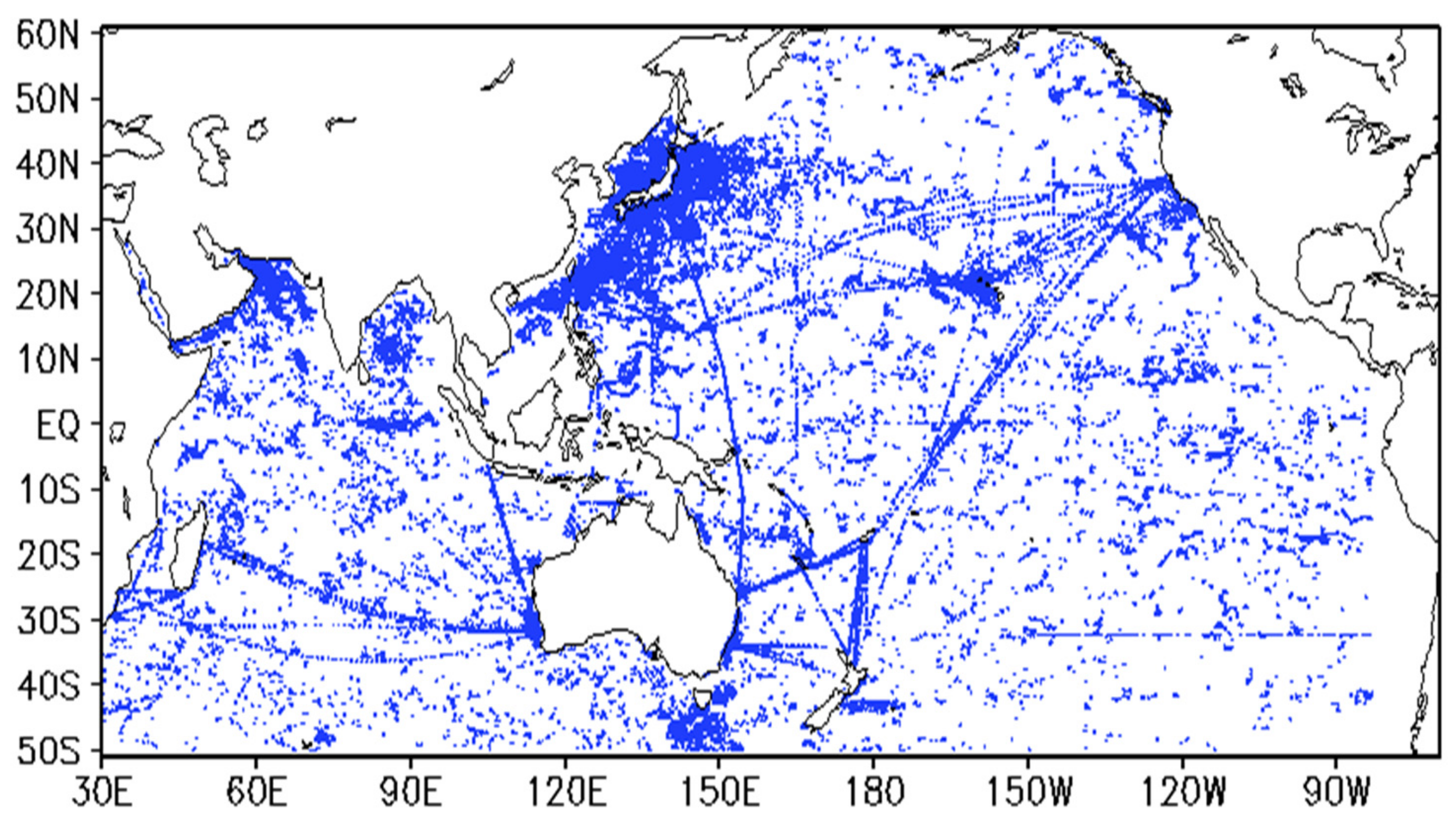
To further verify the accuracy of IPORA, the remaining temperature and salinity profiles after removing super-observations are used for comparison. These profiles are independent observations since they are not used in the IPORA. More than 200,000 profiles are not assimilated during the period 2010–2011 (Figure 3). The withheld observations are mainly distributed in the open sea, especially the north-western Pacific, while they are scarce in coastal regions. Figure 4 shows the vertical profiles of the RMSEs of temperature and salinity in different regions, respectively. It is clear that the fit to the temperature observations is improved in IPORA in terms of RMSEs, the improvement being most significant in the mixed layer and thermocline compared with the control experiment without assimilation in the Indian and Pacific oceans. Similar to temperature, the assimilation also distinctly improves the fit to the salinity observations in the entire upper 700 m. For salinity, the largest RMSEs occur at the sea surface, which is possibly associated with inaccurate fresh-water fluxes and mixing parameterisation. Overall, the RMSEs of IPORA are consistently smaller than those of CNTL for temperature and salinity. Moreover, the assimilation reduces the RMSEs in CTNL by about 44% for temperature and by about 33% for salinity. It indicates the advantages of assimilation. We also calculate the RMSEs of ECCO and SODA using the monthly mean data corresponding to the same temperature and salinity observations. The fit of SODA to the observations is better than IPORA, while ECCO is worse than IPORA. Possibly, the observations used for computing RMSEs are assimilated in SODA, which helps to reduce the RMSEs. Additionally, we also examine the performance of IPORA in different ocean basins. It is obvious that the modelled RMSEs of salinity in CNTL are visibly larger in the Indian Ocean than in the Pacific Ocean. Similarly, the assimilation may greatly reduce the RMSEs, but does not change the pattern with larger RMSEs in the Indian Ocean than in the Pacific Ocean. Both ECCO and SODA also present the same pattern. This result is probably associated with fresh-water fluxes and model configurations (e.g., the vertical parameterisation scheme and vertical and horizontal resolution) in the Indian Ocean. Particularly, the Bay of Bengal, being a part of the Indian Ocean, is affected by complicated factors such as precipitation, runoff, heating, winds, and currents, which induces a low-salinity surface layer to form and strong interannual variabilities of sea surface salinity. Therefore, the salinity in the Bay of Bengal is sensitive to forcing factors. These inaccurate factors can cause large errors. In both ocean basins, SODA still performs best with the smallest RMSEs for temperature. For salinity, there is little difference between IPORA and SODA in the Indian Ocean.
3.3. Sea Level
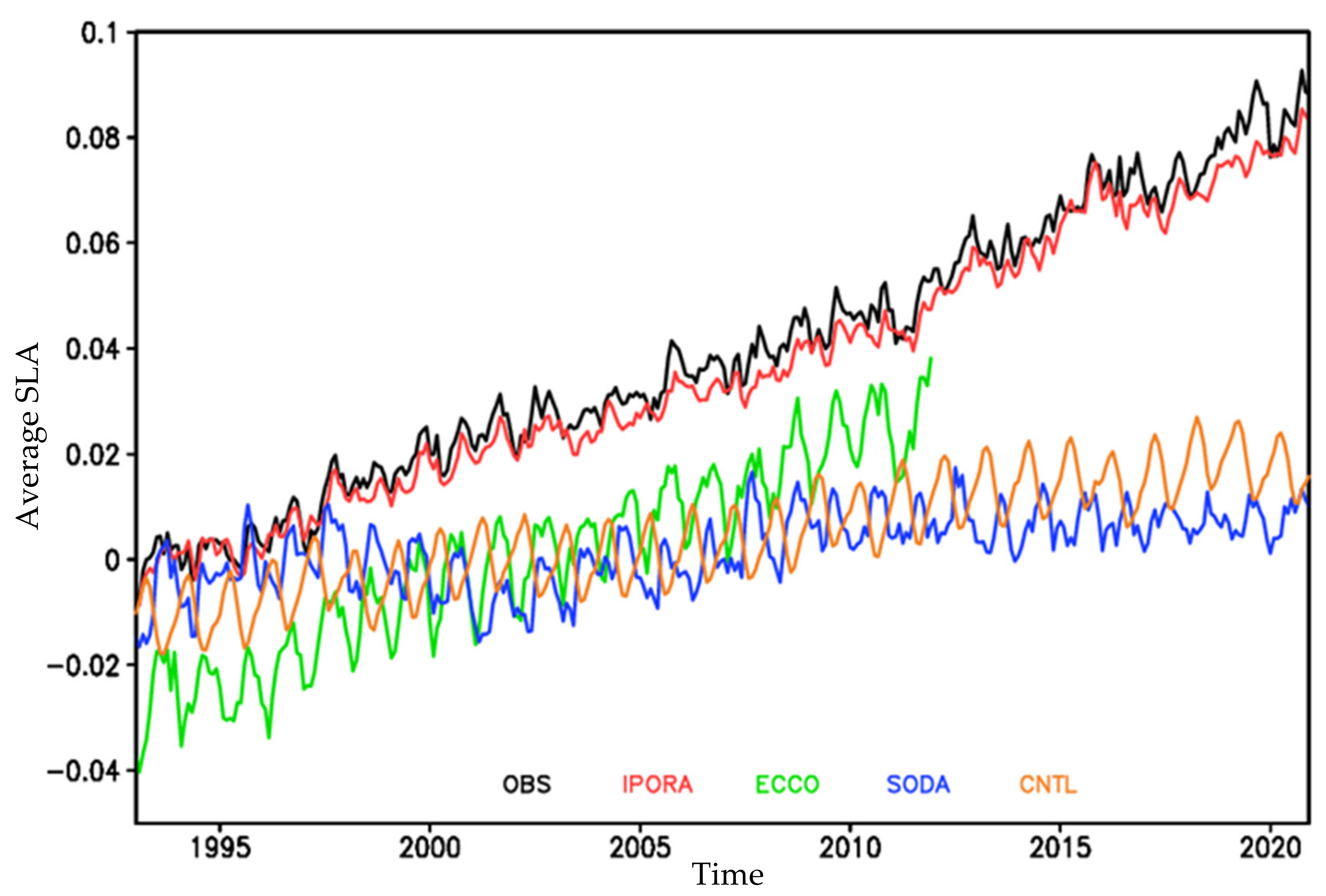
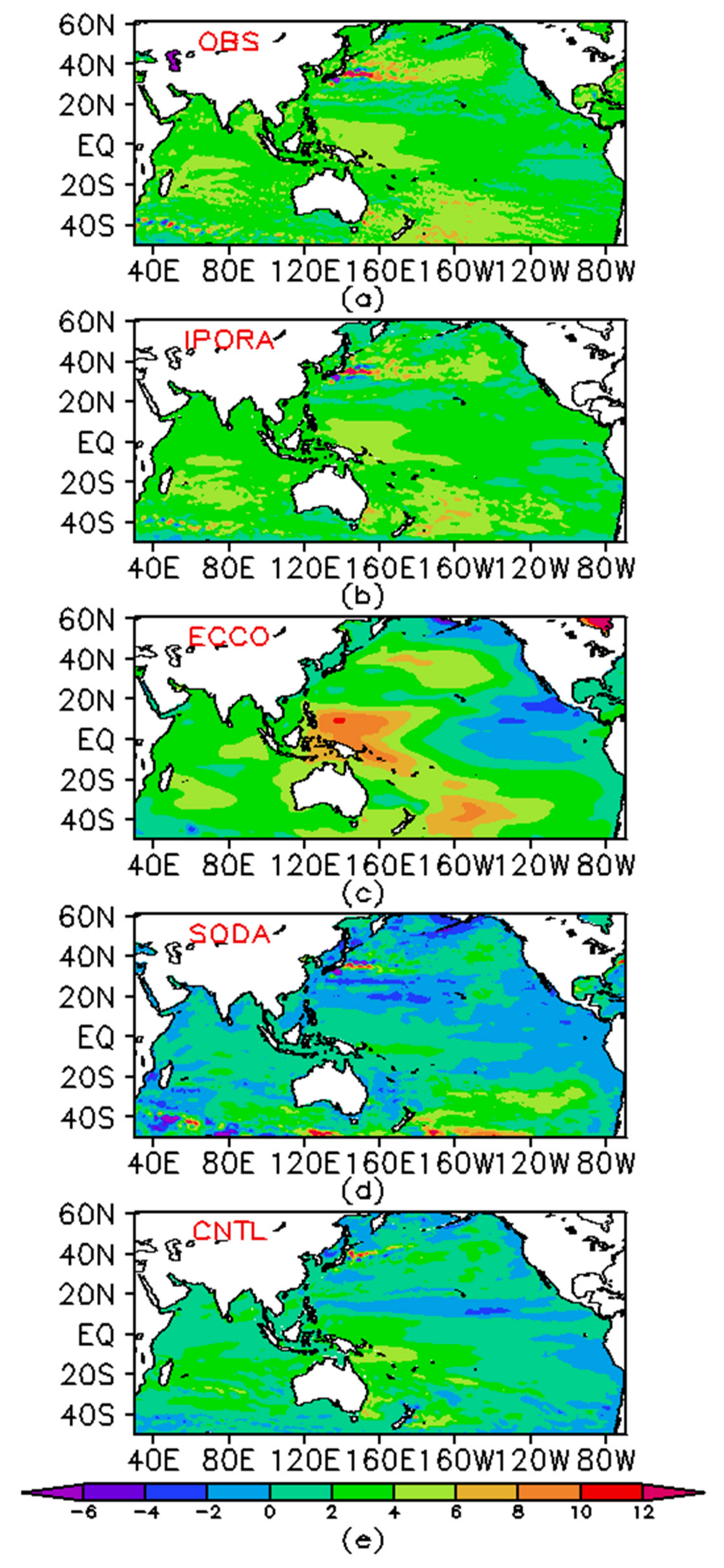
We next evaluated the IPORA data using the monthly mean SLA data during the period of 1993–2020. Figure 5 shows the time series of the average SLA estimated from the CMEMS dataset, CNTL, IPORA, ECCO, and SODA in the Indian and Pacific oceans. The average SLA from IPORA agrees with the observations well and presents a noticeably rising trend during the period of 1993–2020. The SLA from the control experiment without any assimilation also gradually increases with time, but the uptrend is not at all pronounced. The upward trend can be observed in ECCO, but the average SLA is prominently less than the observation. Note that no trend in SLA can be found in SODA. To explore the reason, we computed the linear trend in SLA over the past 28 years from the observations and analyses (Figure 6). It can be seen from the observations that the spatial distribution of the trend in SLA is not uniform. The mixture of significantly increasing and decreasing trends is observed along the path of the Kuroshio Extension and Antarctic Circumpolar Current. These complex phenomena are associated with active eddies. The western Pacific south of 18° N presents a relatively strong increase in SLA. In general, the SLA is basically increasing in the whole Indian and Pacific oceans, except a sporadic weak decrease in the Pacific. IPORA captures the primary features of the observed trend and demonstrates a spatial distribution and strength in the SLA trend similar to the observations. For the control experiment without assimilation, the complicated trend is not present or not evident in the regions with eddies. Although the increasing trend is observed in most regions, the signals are not strong enough. As a result, the uptrend in the region-averaged SLA from CNTL is not obvious. Similarly, a mixture of increased and decreased SLA cannot be found in ECCO. ECCO also shows an increase in SLA in most regions. However, both increase and decrease in SLA are more significant than the observations in the Pacific. Therefore, the resultant SLA averaged over the model domain has a pronounced uptrend for ECCO. SODA shows a notable decrease with extensive coverage and a notable increase to the south of 40° S, which are different from the observations. The resultant average SLA has no trend.
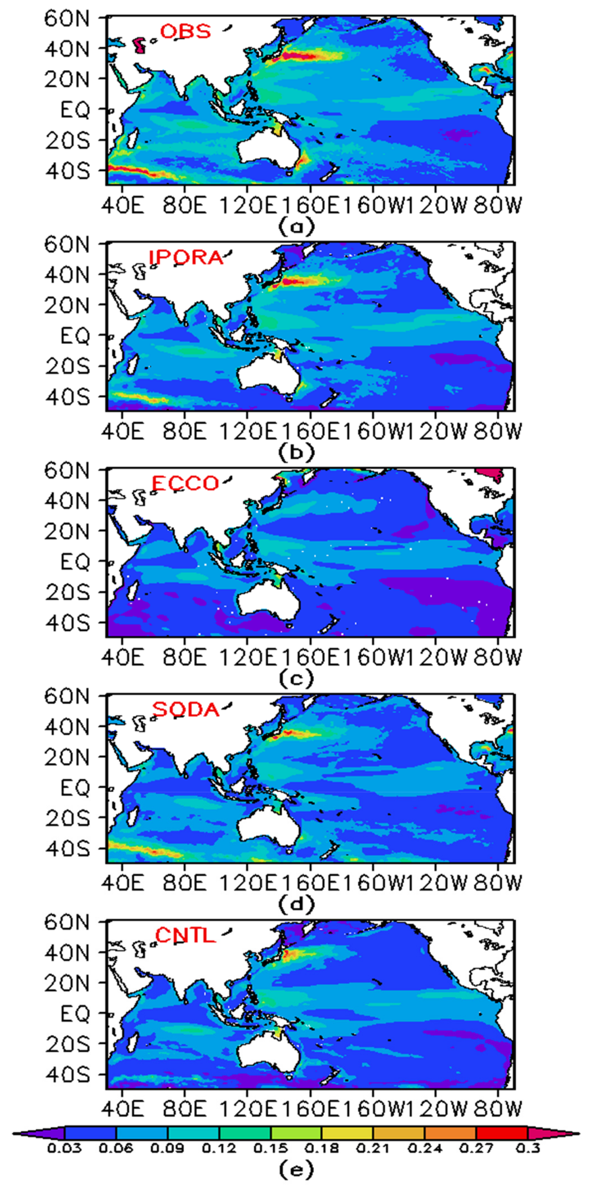
We also examined the variability of SLA for the period 1993–2020. The standard variance of SLA during the period of 1993–2020 is computed from the altimetry data, IPORA, CNTL, ECCO, and SODA (Figure 7). The variance of SLA is actually representative of the eddy kinetic energy. It indicates that a good representative of eddies is very important for an accurate reproduction of SLA variability. It can be seen that the altimetry data present large variability of SLA in the Kuroshio Extension, Agulhas, and East Australian Current regions. As known, these areas are characterised by plentiful eddies. IPORA shows good agreement with the observations by reproducing almost all of the strong signals in the observations. The SLA variability in CNTL is much lower than in IPORA, which can be taken as an indication of the effect of assimilation in reducing uncertainty. SODA, with a resolution of 0.25° × 0.25°, also captures local strong SLA variability, but the magnitude is a little weak in the Kuroshio region compared with IPORA. ECCO greatly underestimates the variability so that it misses local strong signals in the observations. ECCO used here has a 0.5° × 0.5° horizontal resolution, so some mesoscale eddies are not resolved well. Thus, the signals concerned with eddies are not captured well.
3.4. Current Field
To examine the performance of IPORA, the current field of IPORA is compared with the observations. The velocity information is not assimilated in the IPORA, allowing us to use this variable to carry out independent comparisons.
The Ocean Surface Current Analysis Real-time (OSCAR) project provides analyses of global ocean surface currents computed from satellite datasets [51]. Additionally, the Tropical Atmosphere Ocean (TAO)/TRITON array, the Research Moored array for African-Asian-Australian Monsoon Analysis and Prediction (RAMA), and Acoustic Doppler Current Profilers (ADCPs) provide vertical profiles of currents for the tropical oceans which are available from the TAO/RAMA Project office of NOAA/PMEL’s website. These current data and reanalysis products such as SODA and ECCO are used to validate the IPORA data.
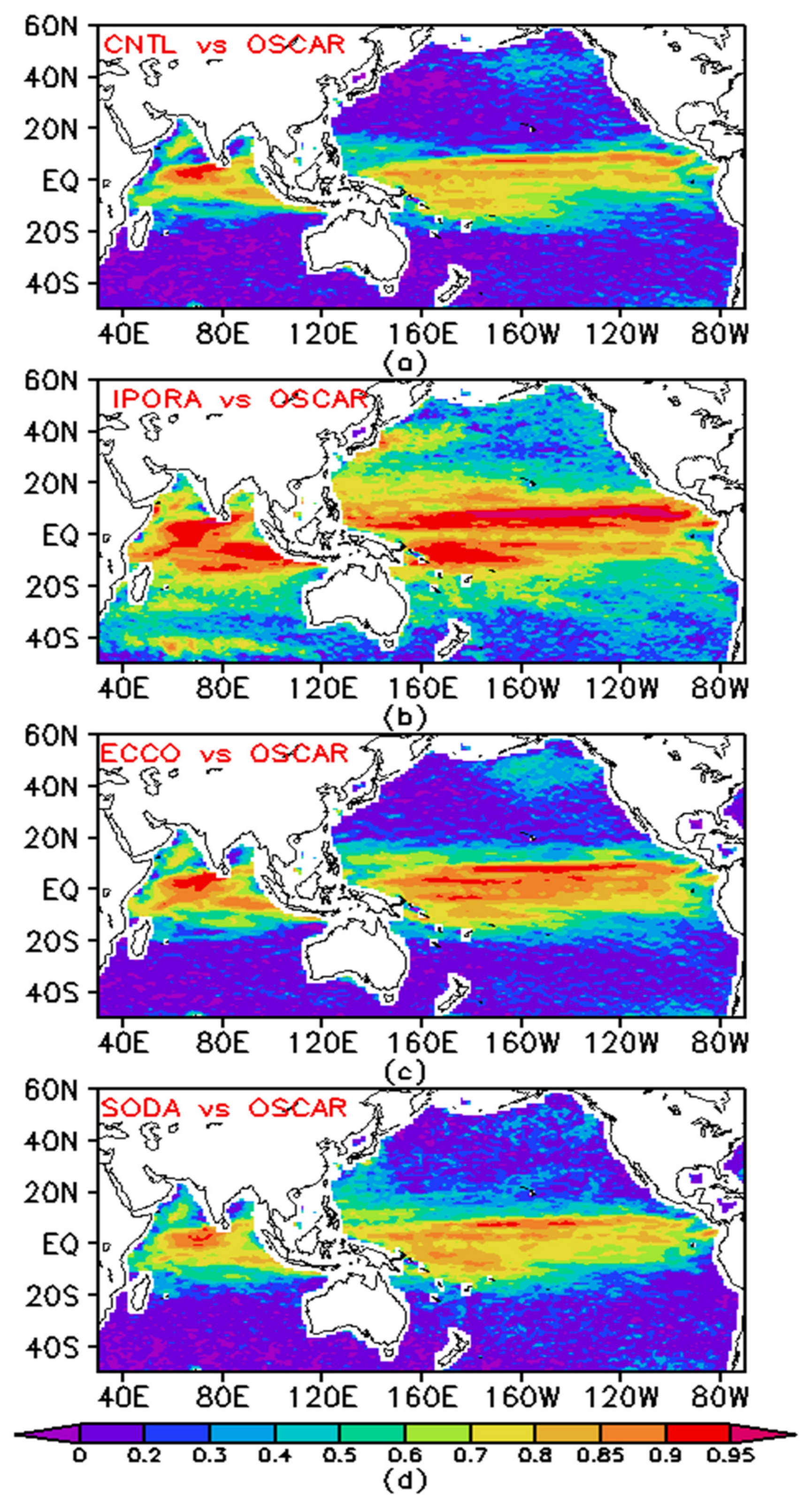
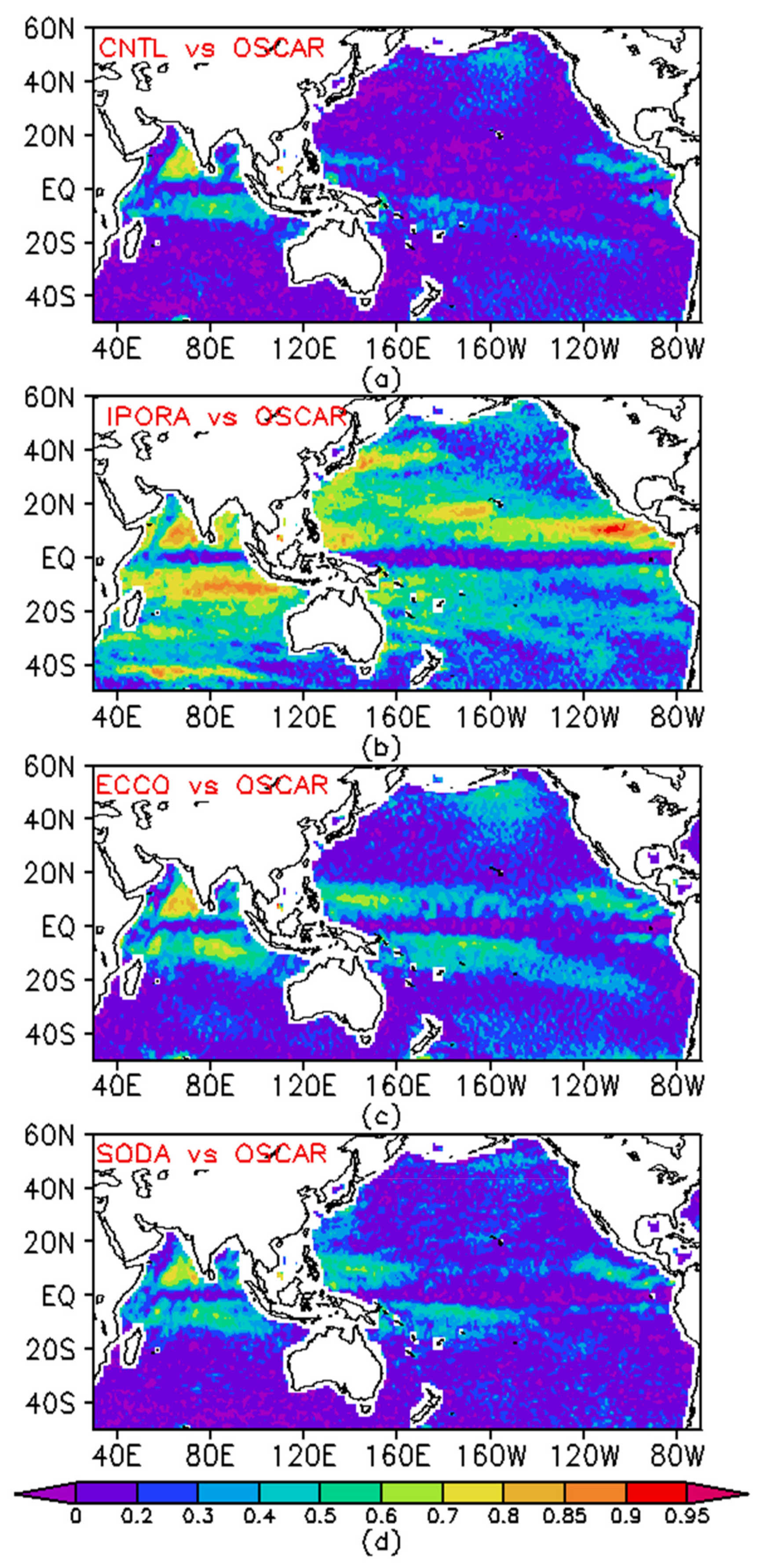
Figure 8 shows the time correlation between the zonal current from OSCAR and the CNTL, IPORA, ECCO, and SODA analyses. For these analyses, the high correlation coefficients with OSCAR are mainly concentrated in the tropical Indian and Pacific oceans within 20° of the equator. It is obvious that IPORA has higher correlation values than CNTL throughout the entire model domain. This result indicates that the assimilation may greatly increase the positive correlation. Moreover, IPORA presents higher correlation coefficients with OSCAR compared to ECCO and SODA. In the equatorial central-eastern Pacific Ocean (0° N–10° N), the correlation values from IPORA are larger than 0.95, while they are smaller for ECCO and SODA. In the southern tropical Indian and Pacific oceans (20° S–0° N), IPORA demonstrates high correlation values larger than 0.9, while ECCO and SODA present lower values. IPORA also exhibits high correlation values in the regions with rich eddies such as the Kuroshio Extension and Agulhas, while they are not observed for ECCO and SODA. Overall, IPORA presents a wider coverage with high correlation than ECCO and SODA do. Figure 9 shows the correlation with OSCAR meridional currents from CNTL, IPORA, ECCO, and SODA data. Noticeably, the higher correlation coefficients from IPORA than those from ECCO, SODA, and CTNL are observed in the model domain. Compared with CNTL, IPORA greatly improves the correlation with OSCAR meridional currents in the Indian and Pacific oceans, except the equatorial regions. It highlights the benefits of the data assimilation. For ECCO and SODA, the good correlation with OSCAR meridional currents is mainly distributed in the tropical oceans (20° S–20° N) apart from the equatorial regions, while IPORA exhibits high correlation in most of the model domain. ECCO presents slightly better correlation with OSCAR zonal and meridional currents than SODA does. CNTL performs worst.
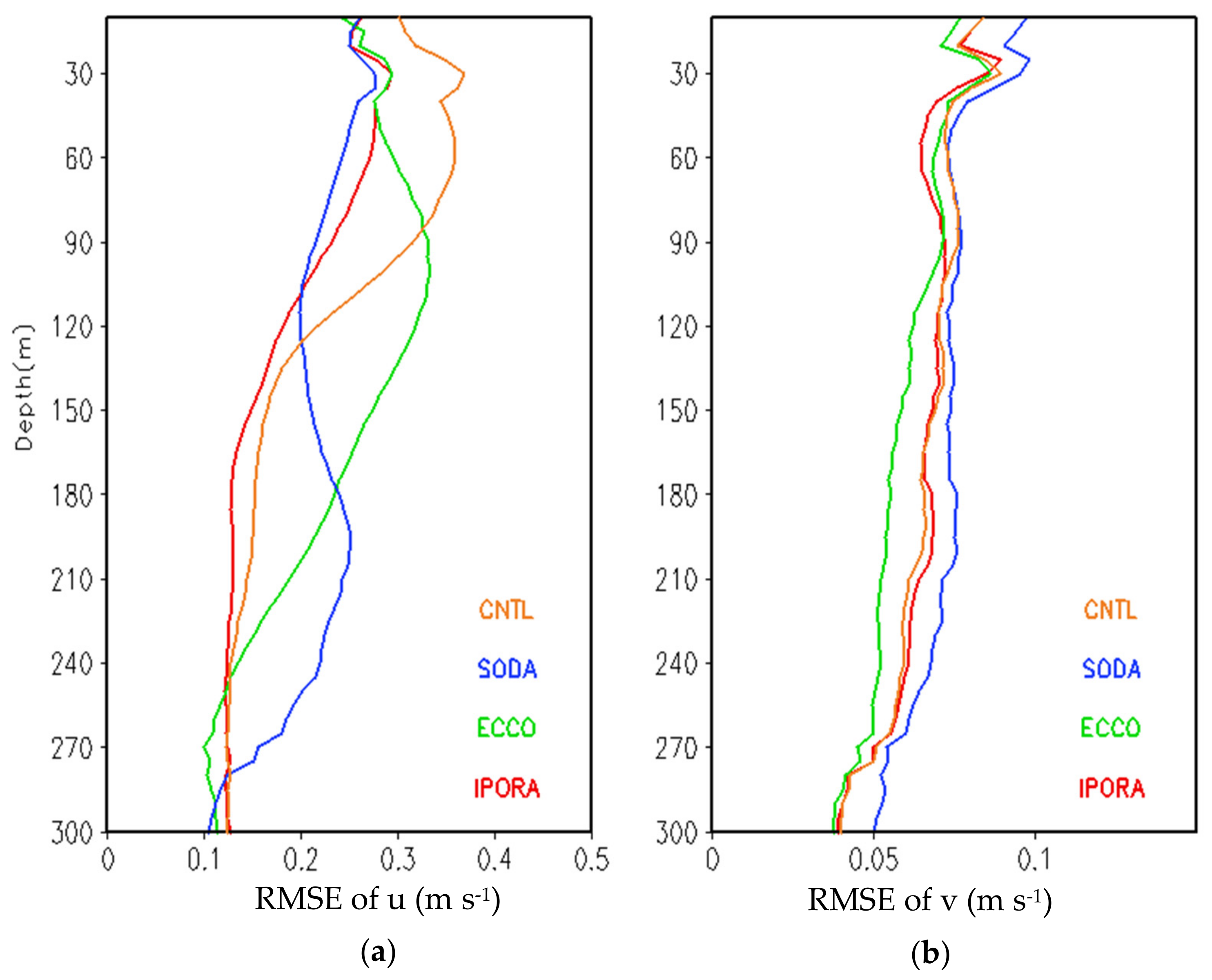
Figure 10 shows the vertical distribution of the RMSEs of the zonal and meridional currents from IPORA, CNTL, ECCO, and SODA with respect to ADCP data over five TAO moorings at positions (0° N, 147° E), (0° N, 165° E), (0° N, 170° W), (0° N, 140° W), and (0° N, 110° W), and two RAMA moorings at (0° N, 80.5° E) and (0° N, 90° E). For the zonal currents, different analyses show different vertical distribution. The RMSEs of IPORA are typically smaller than those of CNTL. Both CNTL and IPORA have similar distribution with large RMSEs (>0.2 m s−1) in the upper 100 m and small RMSEs below. However, the maximum RMSE from CNTL reaches 0.35 m s−1 at 30 m and is notably greater than that of IPORA (0.28 m s−1). ECCO exhibits a peak RMSE of 0.33 m s−1 at a depth of 105 m and relatively large RMSEs (>0.2 m s−1) in the upper 200 m. IPORA, CNTL, and ECCO have one peak RMSE. Note that SODA demonstrates two peak RMSEs (around 0.27 and 0.25 m s−1, respectively) at depths of 40 m and 200 m. On average, IPORA presents the smallest RMSE of 0.18 m s−1 and ECCO shows the largest RMSE of 0.23 m s−1, while both CNTL and SODA present a RMSE of 0.21 m s−1. Compared with the zonal currents, the RMSEs of meridional currents are much smaller. The maximum RMSE for meridional currents is smaller than 0.1 m s−1, while the minimum RMSE for zonal currents is larger than 0.1 m s−1. It is evident that SODA shows the largest RMSEs among all analyses in the upper 300 m for meridional currents. ECCO presents the smallest RMSEs in the upper 30 m and below 90 m. IPORA slightly outperforms CNTL. In general, SODA performs worst with a RMSE of 0.073 m s−1, and ECCO performs best with a RMSE of 0.06 m s−1, while it is 0.065 m s−1 for IPORA and 0.066 m s−1 for CNTL. In fact, these differences in meridional currents among analyses are relatively small.
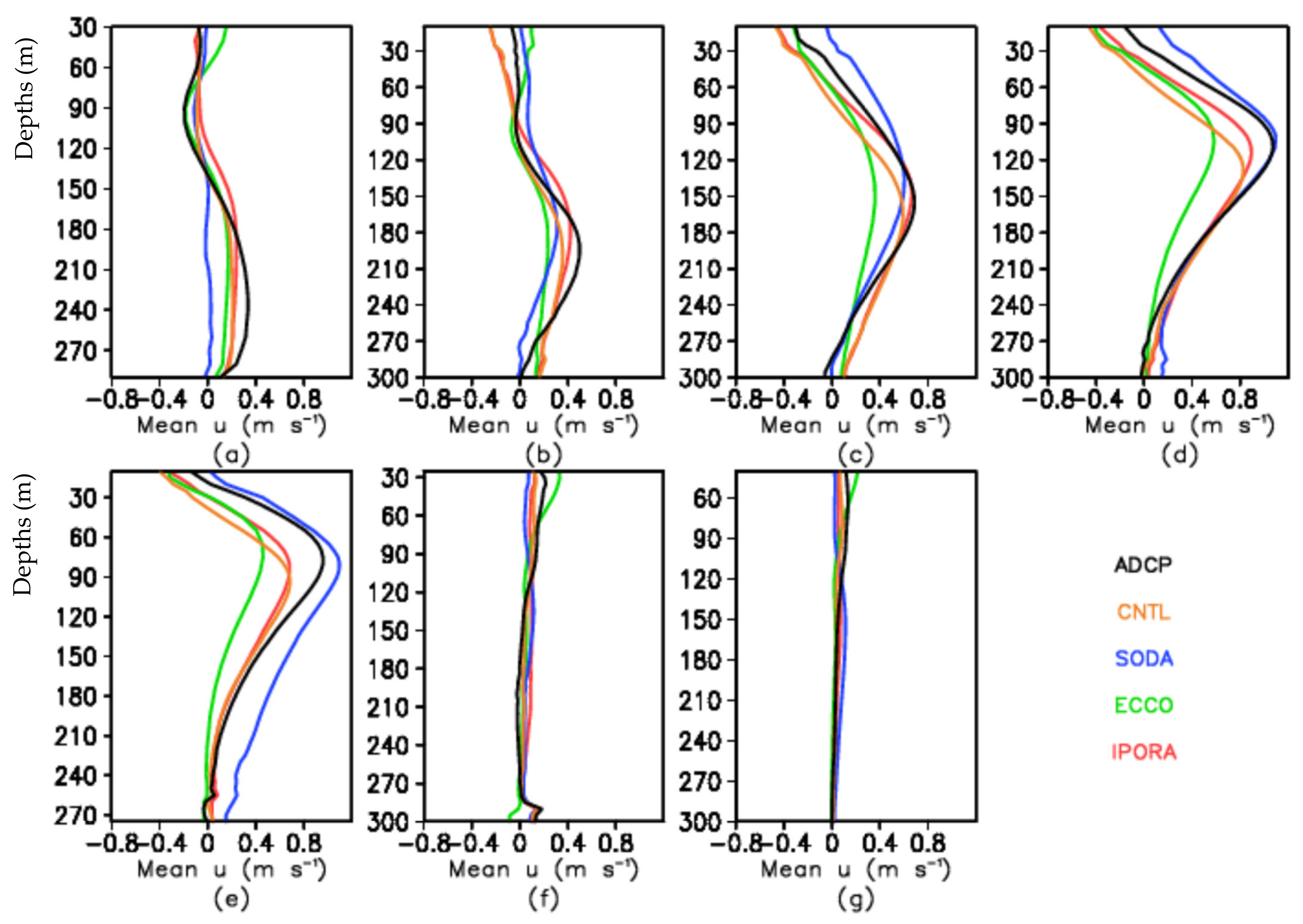
Figure 11 shows the temporal mean profiles of the zonal currents from ADCP data, CNTL, IPORA, ECCO, and SODA for seven moorings in the TAO/RAMA array. It can be seen from the observations that from the western Pacific to the eastern Pacific, the depth of the peak speed of the eastward equatorial undercurrent gradually shallows from 230 m to 80 m, and the peak speed gradually strengthens. All analyses reconstruct this pattern of the undercurrent. Compared with CNTL, IPORA distinctly improves the strength of the equatorial undercurrent in the Pacific Ocean. The undercurrent from ECCO is basically the weakest among analyses, which results in large RMSEs of zonal currents. It is probably associated with the diffuse thermocline (Figure 4) from ECCO. In the eastern Pacific (140° W and 110° W), compared with the observations, the undercurrent from SODA is slightly strong, while those from IPORA, CNTL, and ECCO are too weak. However, IPORA is better than CNTL and ECCO. Meanwhile, the surface western currents are too strong in the analyses with the exception of SODA. Actually, the mean surface current in SODA flows eastward, which is different from the observations. In the central and western Pacific (147° E and 165° E), the undercurrent from all analyses is weaker than the observations, especially SODA. It is why SODA also has a peak RMSE at 200 m shown as Figure 10. IPORA presents a stronger undercurrent than other analyses do. In the Indian Ocean, there is not obvious undercurrent, and there is little difference in the mean current profiles from all analyses.
4. Discussion and Conclusions
In this study, we have produced an ocean reanalysis IPORA for the Indian and Pacific oceans over 28 years. IPORA uses the EnOI-based schemes to assimilate data from in-situ temperature and salinity, gridded SST, and altimeter-derived SLA observations into HYCOM. A long-term assimilation experiment was conducted using the ERA-interim atmospheric forcing to produce the reanalysis dataset during the period of 1993–2020.
An ocean model simulation without assimilating data was implemented as a control experiment to evaluate the quality of IPORA. We assessed the IPORA data by a variety of qualitative and quantitative comparisons with satellite data, independent temperature and salinity profiles, and observed current fields, as well as other reanalyses (e.g., ECCO and SODA).
Through the comparisons with the control experiment, IPORA consistently improves the fit to observations of SST, temperature and salinity, SLA, and currents in the Indian and Pacific oceans. The RMSEs in IPORA are significantly reduced, especially at the thermocline. Moreover, the interannual variability of the ocean estimate is also greatly improved in IPORA, as suggested by the improved standard variance of SLA and the improved temporal correlation with surface current fields. The growing tendency in SLA is reproduced better by IPORA. In comparison with ECCO and SODA, IPORA also exhibits a better agreement with the altimetry data, OSCAR, and ADCP. On the one hand, it is partly associated with the model resolution. On the other hand, it is also related to the assimilation method for SLA. IPORA is potentially a valuable dataset for better understanding of a variety of ocean research topics.
Although IPORA demonstrates reduced RMSEs for the zonal current, there is still discrepancy in the representative of the equatorial undercurrent in contrast with the ADCP data. The undercurrent is too shallow in the central-western Pacific, and it is too weak despite it being strengthened by the assimilation. Moreover, it is also observed in ECCO and SODA. It is a common feature for most ocean simulations and reanalyses. The robustness of this signal is probably associated with the model configurations, the wind stress, changes in SST, as well as other forcing fields. It will be investigated in future work.
Author Contributions
Conceptualization, C.Y. and J.Z.; methodology, J.Z. and C.Y.; data collection and treatment, C.Y.; software, C.Y. and J.Z.; experiment setup, C.Y.; validation, C.Y. and J.Z.; result analysis, C.Y. and J.Z.; writing—original draft preparation, C.Y.; writing—review and editing, C.Y. and J.Z.; discussion and conclusion, J.Z. and C.Y. All authors have read and agreed to the published version of the manuscript.
Funding
This research was funded by the Strategic Priority Research Program of Chinese Academy of Sciences, grant number XDA19060102 and XDB42040106, the National Natural Science Foundation of China, grant number 41776041.
Institutional Review Board Statement
Not applicable.
Informed Consent Statement
Not applicable.
Data Availability Statement
Not applicable.
Acknowledgments
The authors would like to thank CMEMS, Met Office Hadley Centre, and RAMA/TAO project Office of NOAA/PMEL for the provided data.
Conflicts of Interest
The authors declare no conflict of interest.
References
- Kalnay, E.; Kalnay, E.; Kanamitsu, M.; Kistler, R.; Collins, W.; Deaven, D.; Gandin, L.; Iredell, M.; Saha, S.; White, G.; et al. The NCEP/NCAR 40-Year Reanalysis Project. Bull. Amer. Meteor. Soc. 1996, 77, 437–471. [Google Scholar] [CrossRef]
- Carton, J.A.; Chepurin, G.; Cao, X.; Giese, B.S. A Simple Ocean Data Assimilation analysis of the global upper ocean 1950–95. Part I: Methodology. J. Phys. Oceanogr. 2000, 30, 294–309. [Google Scholar] [CrossRef]
- Carton, J.A.; Chepurin, G.; Cao, X. A Simple Ocean Data Assimilation analysis of the global upper ocean 1950–95. Part II: Results. J. Phys. Oceanogr. 2000, 30, 311–326. [Google Scholar] [CrossRef]
- Xie, J.; Counillon, F.; Zhu, J.; Bertino, L. An eddy resolving tidal-driven model of the South China Sea assimilating along-track SLA data using the EnOI. Ocean Sci. 2011, 7, 609–627. [Google Scholar] [CrossRef] [Green Version]
- Oke, P.R.; Griffin, D.; Schiller, A.; Matear, R.J.; Fiedler, R.; Mansbridge, J.; Lenton, A.; Cahill, M.; Chamberlain, M.A.; Ridgway, K. Evaluation of a near-global eddy-resolving ocean model. Geosci. Model Dev. 2013, 6, 591–615. [Google Scholar] [CrossRef] [Green Version]
- Masina, S.; Storto, A.; Ferry, N.; Valdivieso, M.; Haines, K.; Balmaseda, M.A.; Zuo, H.; Drevillon, M.; Parent, L. An ensemble of eddy-permitting global ocean reanalyses from the MyOcean project. Clim. Dyn. 2017, 49, 813–841. [Google Scholar] [CrossRef] [Green Version]
- Carton, J.A.; Chepurin, G.; Chen, L. SODA3: A new ocean climate reanalysis. J. Clim. 2018, 31, 6967–6983. [Google Scholar] [CrossRef]
- Balmaseda, M.A.; Vidard, A.; Anderson, D.L.T. The ECMWF Ocean Analysis System: ORA-S3. Mon. Weather. Rev. 2008, 136, 3018–3034. [Google Scholar] [CrossRef]
- Balmaseda, M.A.; Mogensen, K.; Weaver, A.T. Evaluation of the ECMWF ocean reanalysis system ORAS4. Q. J. Roy. Meteor. Soc. 2013, 139, 1132–1161. [Google Scholar] [CrossRef]
- Speer, K.; Forget, G. Global distribution and formation of mode waters. Chapter 9. In Ocean Circulation and Climate—A 21st Century Perspective; International Geophysics Series; Sielder, G., Church, J., Griffes, S., Gould, J., Church, J., Eds.; Academic Press: Cambridge, MA, USA; Elsevier: Amsterdam, The Netherlands, 2013; Volume 103, ISBN 978-0-12-391851-2. [Google Scholar]
- Wunsch, C.; Heimbach, P. Dynamically and Kinematically Consistent Global Ocean Circulation and Ice State Estimates. Chapter 21. In Ocean Circulation and Climate—A 21st Century Perspective; International Geophysics Series; Sielder, G., Church, J., Griffes, S., Gould, J., Church, J., Eds.; Academic Press: Cambridge, MA, USA; Elsevier: Amsterdam, The Netherlands, 2013; Volume 103, ISBN 978-0-12-391851-2. [Google Scholar]
- Fujii, Y.; Nakaegawa, N.; Matsumoto, S.; Yasuda, T.; Yamanaka, G.; Kamachi, M. Coupled climate simulation by constraining ocean fields in a coupled model with ocean data. J. Clim. 2009, 22, 5541–5557. [Google Scholar] [CrossRef]
- Toyoda, T.; Fujii, Y.; Yasuda, T.; Usui, N.; Iwao, T.; Kuragano, T.; Kamachi, M. Improved analysis of the seasonal interannual fields by a global ocean data assimilation system. Theor. Appl. Mech. Jpn. 2013, 61, 31–48. [Google Scholar]
- Tsujino, H.; Hirabara, M.; Nakano, H.; Yasuda, T.; Motoi, T.; Yamanaka, G. Simulating present climate of the global ocean-ice system using the Meteorological Research Institute Community Ocean Model (MRI.COM): Simulation characteristics and variability in the Pacific sector. J. Oceanogr. 2011, 67, 449–479. [Google Scholar] [CrossRef]
- Danabasoglu, G.; Yeager, S.G.; Bailey, D.; Behrens, E.; Bentsen, M.; Bi, D.; Biastoch, A.; Böning, C.; Bozec, A.; Canuto, V.M.; et al. North Atlantic simulations in Coordinated Ocean-ice Reference Experiments phase II (CORE-II). Part I: Mean states. Ocean Model. 2014, 73, 76–107. [Google Scholar] [CrossRef] [Green Version]
- Sakov, P.; Counillon, F.; Bertino, L.; Lisæther, K.A.; Oke, P.R.; Korablev, A. TOPAZ4: An ocean-sea ice data assimilation system for the North Atlantic and Arctic. Ocean Sci. 2012, 8, 633–656. [Google Scholar] [CrossRef] [Green Version]
- Xie, J.; Bertino, L.; Counillon, F.; Lisæter, K.A.; Sakov, P. Quality assessment of the TOPAZ4 reanalysis in the Arctic over the period 1991–2013. Ocean Sci. 2017, 13, 123–144. [Google Scholar] [CrossRef] [Green Version]
- Han, G.; Li, W.; Zhang, X.; Li, D.; He, Z.; Wang, X.; Wu, X.; Yu, T.; Ma, J. A regional ocean reanalysis system for coastal waters of china and adjacent seas. Adv. Atmos. Sci. 2011, 28, 682–690. [Google Scholar] [CrossRef]
- Han, G.; Fu, H.; Zhang, X.; Li, W.; Wu, X.; Wang, X.; Zhang, L. A global ocean reanalysis product in the China Ocean Reanalysis (CORA) project. Adv. Atmos. Sci. 2013, 30, 1621–1631. [Google Scholar] [CrossRef]
- Usui, N.; Wakamatsu, T.; Tanaka, Y.; Hirose, N.; Toyoda, T.; Nishikawa, S.; Fujii, Y.; Takatsuki, Y.; Igarashi, H.; Nishikawa, H.; et al. Four-dimensional variational ocean reanalysis: A 30-year high-resolution dataset in the western North Pacific (FORA-WNP30). J. Oceanogr. 2017, 73, 205–233. [Google Scholar] [CrossRef] [Green Version]
- Dwivedi, S.; Srivastava, A.; Mishra, A.K. Upper Ocean Four-Dimensional Variational Data Assimilation in the Arabian Sea and Bay of Bengal. Mar. Geod. 2018, 41, 230–257. [Google Scholar] [CrossRef]
- Karmakar, A.; Parekh, A.; Chowdary, J.S.; Gnanaseelan, C. Inter comparison of Tropical Indian Ocean features in different ocean reanalysis products. Clim. Dyn. 2018, 51, 119–141. [Google Scholar] [CrossRef]
- Fukumori, I. A partitioned Kalman filter and smoother. Mon. Wea. Rev. 2002, 130, 1370–1383. [Google Scholar] [CrossRef]
- Behringer, D. The global ocean data assimilation system at NCEP. Preprints, 11th Symp. on Integrated Observing and Assimilation Systems for Atmosphere, Oceans, and Land Surface, San Antonio, TX, Amer. Meteor. Soc. 3.3. 2007. Available online: http://ams.confex.com/ams/pdfpapers/119541.pdf (accessed on 9 December 2022).
- Saha, S.; Moorthi, S.; Pan, H.; Wu, X.; Wang, J.; Nadiga, S.; Tripp, P.; Kistler, R.; Woollen, J.; Behringer, D.; et al. The NCEP climate forecast system reanalysis. Bull. Am. Meteorol. Soc. 2010, 91, 1015–1057. [Google Scholar] [CrossRef] [Green Version]
- Balmaseda, M.A.; Hernandez, F.; Storto, A.; Palmer, M.D.; Alves, O.; Shi, L.; Smith, G.C.; Toyoda, T.; Valdivieso, M.; Barnier, B.; et al. The Ocean Reanalyses Intercomparison Project (ORA-IP). J. Oper. Oceanogr. 2015, 7, 81–99. [Google Scholar] [CrossRef]
- Xue, Y.; Huang, B.; Hu, Z.; Kumar, A.; Wen, C.; Behringer, D.; Nadiga, S. An Assessment of Oceanic Variability in the NCEP Climate Forecast System Reanalysis. Clim. Dyn. 2011, 37, 2511–2539. [Google Scholar] [CrossRef]
- Carton, J.A.; Penny, S.G.; Kalnay, E. Temperature and salinity variability in soda3, ECCO4r3, and ORAS5 ocean reanalyses, 1993-2015. J. Clim. 2019, 32, 2277–2293. [Google Scholar] [CrossRef]
- Lellouche, J.-M.; Greiner, E.; Le Galloudec, O.; Garric, G.; Regnier, C.; Drevillon, M.; Benkiran, M.; Testut, C.; Bourdalle-Badie, R.; Gasparin, F.; et al. Recent updates to the Copernicus Marine Service global ocean monitoring and forecasting real-time 1/12° high-resolution system. Ocean Sci. 2018, 14, 1093–1126. [Google Scholar] [CrossRef] [Green Version]
- Zuo, H.; Balmaseda, M.A.; Mogensen, K. The new eddypermitting ORAP5 ocean reanalysis: Description, evaluation and uncertainties in climate signals. Clim. Dynam. 2017, 49, 791–811. [Google Scholar] [CrossRef]
- Zuo, H.; Balmaseda, M.A.; Tietsche, S.; Mogensen, K.; Mayer, M. The ECMWF operational ensemble reanalysis–analysis system for ocean and sea ice: A description of the system and assessment. Ocean Sci. 2019, 15, 779–808. [Google Scholar] [CrossRef] [Green Version]
- Storto, A.; Masina, S.; Navarra, A. Evaluation of the CMCC eddy-permitting global ocean physical reanalysis system (C-GLORS, 1982-2012) and its assimilation components. Q. J. R. Meteorol. Soc. 2016, 142, 738–758. [Google Scholar] [CrossRef]
- Bleck, R. An oceanic general circulation model framed in hybrid isopycnic-Cartesian coordinates. Ocean Model. 2002, 4, 55–88. [Google Scholar] [CrossRef]
- Chassignet, E.P.; Smith, L.T.; Halliwell, G.R. North Atlantic Simulations with the Hybrid Coordinate Ocean Model (HYCOM): Impact of the vertical coordinate choice, reference pressure, and thermobaricity. J. Phys. Oceanogr. 2003, 33, 2504–2526. [Google Scholar] [CrossRef]
- Bertino, L.; Lisaeter, K.A.; Scient, S. The TOPAZ monitoring and prediction system for the Atlantic and Arctic Oceans. J. Oper. Oceanogr. 2008, 1, 15–18. [Google Scholar] [CrossRef] [Green Version]
- Large, W.G.; McWilliams, J.C.; Doney, S.C. Oceanic vertical mixing: A review and a model with a nonlocal boundary layer parameterization. Rev. Geophys. 1994, 32, 363–403. [Google Scholar] [CrossRef] [Green Version]
- Dee, D.P.; Uppala, S.M.; Simmons, A.J.; Berrisford, P.; Poli, P.; Kobayashi, S.; Andrae, U.; Balmaseda, M.A.; Balsamo, G.; Bauer, P.; et al. The ERA-Interim reanalysis: Configuration and performance of the data assimilation system. Q. J. R. Meteor. Soc. 2011, 137, 553–597. [Google Scholar] [CrossRef]
- Reynolds, R.W.; Smith, T.M.; Liu, C.Y.; Chelton, D.B.; Casey, K.S.; Schlax, M.G. Daily high-resolutionblended analyses for sea surface temperature. J. Clim. 2007, 20, 5473–5496. [Google Scholar] [CrossRef]
- Banzon, V.; Smith, T.M.; Liu, C.; Hankins, W. A longterm record of blended satellite and in situ sea surface temperature for climate monitoring, modeling and environmental studies. Earth Syst. Sci. Data 2016, 8, 165–176. [Google Scholar] [CrossRef] [Green Version]
- Huang, B.; Liu, C.; Banzon, V.; Freeman, E.; Graham, G.; Hankins, B.; Smith, T.; Zhang, H. Improvements of the Daily Optimum Interpolation Sea Surface Temperature (DOISST) Version 2.1. J. Clim. 2020, 34, 2923–2939. [Google Scholar] [CrossRef]
- Ingleby, B.; Huddleston, M. Quality control of ocean temperature and salinity profiles—Historical and real-time data. J. Mar. Syst. 2007, 65, 158–175. [Google Scholar] [CrossRef]
- Cheng, L.; Zhu, J.; Cowley, R.; Boyer, T.; Wijffels, S. Time, Probe Type, and Temperature Variable Bias Corrections to Historical Expendable Bathythermograph Observations. J. Atmos. Ocean. Technol. 2014, 31, 1793–1825. [Google Scholar] [CrossRef]
- Gouretski, V.; Cheng, L. Correction for Systematic Errors in the Global Dataset of Temperature Profiles from Mechanical Bathythermographs. J. Atmos. Technol. Ocean. Res. 2020, 37, 841–855. [Google Scholar] [CrossRef] [Green Version]
- Cummings, J.A. Operational multivariate ocean data assimilation. Q. J. Roy. Met. Soc. 2005, 131, 3583–3604. [Google Scholar] [CrossRef]
- Evensen, G. The Ensemble Kalman Filter: Theoretical formulation and practical implementation. Ocean Dyn. 2003, 53, 343–367. [Google Scholar] [CrossRef]
- Xie, J.; Zhu, J. Ensemble optimal interpolation schemes for assimilating Argo profiles into a hybrid coordinate ocean model. Ocean Model. 2010, 33, 283–298. [Google Scholar] [CrossRef]
- Chen, Y.; Yan, C.; Zhu, J. Assimilation of sea surface temperature in a global Hybrid Coordinate Ocean Model. Adv. Atmos. Sci. 2018, 35, 1291–1304. [Google Scholar] [CrossRef]
- Yan, C.; Zhu, J.; Tanajura, C.A.S. Impacts of mean dynamic topography on a regional ocean assimilation system. Ocean Sci. 2015, 11, 829–837. [Google Scholar] [CrossRef] [Green Version]
- Forget, G.; Campin, J.-M.; Heimbach, P.; Hill, C.N.; Ponte, R.M.; Wunsch, C. ECCO version 4: An integrated framework for non-linear inverse modeling and global ocean state esti-mation. Geosci. Model Dev. 2015, 8, 3071–3104. [Google Scholar] [CrossRef] [Green Version]
- Forget, G.; Campin, J.-M.; Heimbach, P.; Hill, C.N.; Ponte, R.M.; Wunsch, C. ECCO version 4: Second release. 2016. Available online: http://hdl.handle.net/1721.1/102062 (accessed on 1 April 2021).
- Bonjean, F.; Lagerloef, G.S.E. Diagnostic model and analysis of the surface currents in the tropical Pacific Ocean. J. Phys. Oceanogr. 2002, 32, 2938–2954. [Google Scholar] [CrossRef]
Figure 1.
Time series of SST RMSEs (units: °C) in the model domain from CNTL, IPORA, ECCO, and SODA for the period of 1993–2020.
Figure 1.
Time series of SST RMSEs (units: °C) in the model domain from CNTL, IPORA, ECCO, and SODA for the period of 1993–2020.

Figure 2.
RMSEs of SST (units: °C) in the model domain over the period of 1993–2020 from (a) CNTL, (b) IPORA, (c) ECCO, and (d) SODA.
Figure 2.
RMSEs of SST (units: °C) in the model domain over the period of 1993–2020 from (a) CNTL, (b) IPORA, (c) ECCO, and (d) SODA.

Figure 3.
The distribution of temperature and salinity profiles withheld from the assimilation during the period of 2010–2011.
Figure 3.
The distribution of temperature and salinity profiles withheld from the assimilation during the period of 2010–2011.

Figure 4.
The vertical distribution of the RMSEs of temperature (a–c) and salinity (d–f) against the independent profiles over the period 2010–2011 from CNTL, IPORA, ECCO, and SODA in different regions. (a,d) the Indian and Pacific oceans, (b,e) the Pacific Ocean, and (c,f) the Indian Ocean.
Figure 4.
The vertical distribution of the RMSEs of temperature (a–c) and salinity (d–f) against the independent profiles over the period 2010–2011 from CNTL, IPORA, ECCO, and SODA in different regions. (a,d) the Indian and Pacific oceans, (b,e) the Pacific Ocean, and (c,f) the Indian Ocean.

Figure 5.
Time series of the average SLA (units: m) from the observations, CNTL, IPORA, ECCO, and SODA in the Indian and Pacific oceans.
Figure 5.
Time series of the average SLA (units: m) from the observations, CNTL, IPORA, ECCO, and SODA in the Indian and Pacific oceans.

Figure 6.
The linear trend (units: mm yr−1) of SLA during the period of 1993–2020 in the Indian and Pacific oceans from (a) observations, (b) IPORA, (c) ECCO, (d) SODA, and (e) CNTL.
Figure 6.
The linear trend (units: mm yr−1) of SLA during the period of 1993–2020 in the Indian and Pacific oceans from (a) observations, (b) IPORA, (c) ECCO, (d) SODA, and (e) CNTL.

Figure 7.
The standard variance of SLA (units: m) during the period of 1993–2020 in the Indian and Pacific oceans from (a) observations, (b) IPORA, (c) ECCO, (d) SODA, and (e) CNTL.
Figure 7.
The standard variance of SLA (units: m) during the period of 1993–2020 in the Indian and Pacific oceans from (a) observations, (b) IPORA, (c) ECCO, (d) SODA, and (e) CNTL.

Figure 8.
Time correlation with OSCAR surface zonal currents from (a) CNTL, (b) IPORA, (c) ECCO, and (d) SODA for the period of 1993–2011.
Figure 8.
Time correlation with OSCAR surface zonal currents from (a) CNTL, (b) IPORA, (c) ECCO, and (d) SODA for the period of 1993–2011.

Figure 9.
Time correlation with OSCAR surface meridional currents from (a) CNTL, (b) IPORA, (c) ECCO, and (d) SODA for the period of 1993–2011.
Figure 9.
Time correlation with OSCAR surface meridional currents from (a) CNTL, (b) IPORA, (c) ECCO, and (d) SODA for the period of 1993–2011.

Figure 10.
Vertical distribution of the RMSEs of zonal (a) and meridional (b) currents from CNTL, SODA, ECCO, and IPORA with respect to the ADCP data over seven moorings in the TAO/RAMA array.
Figure 10.
Vertical distribution of the RMSEs of zonal (a) and meridional (b) currents from CNTL, SODA, ECCO, and IPORA with respect to the ADCP data over seven moorings in the TAO/RAMA array.

Figure 11.
Temporal mean vertical profiles of the zonal current at seven moorings in the TAO/RAMA array compared with CNTL, IPORA, ECCO, and SODA. (a) (0° N, 147° E), (b) (0° N, 165° E), (c) (0° N, 170° W), (d) (0° N, 140° W), (e) (0° N, 110° W), (f) (0° N, 80.5° E), and (g) (0° N, 90° E).
Figure 11.
Temporal mean vertical profiles of the zonal current at seven moorings in the TAO/RAMA array compared with CNTL, IPORA, ECCO, and SODA. (a) (0° N, 147° E), (b) (0° N, 165° E), (c) (0° N, 170° W), (d) (0° N, 140° W), (e) (0° N, 110° W), (f) (0° N, 80.5° E), and (g) (0° N, 90° E).


Table 1.
Reanalysis settings.
| Reanalysis Name | Assimilation Method | Assimilated Data | Assimilation Frequency | Period |
|---|---|---|---|---|
| IPORA | EnOI | T/S, SST, SLA | 7 days | 1993–2020 |
Disclaimer/Publisher’s Note: The statements, opinions and data contained in all publications are solely those of the individual author(s) and contributor(s) and not of MDPI and/or the editor(s). MDPI and/or the editor(s) disclaim responsibility for any injury to people or property resulting from any ideas, methods, instructions or products referred to in the content. |
© 2023 by the authors. Licensee MDPI, Basel, Switzerland. This article is an open access article distributed under the terms and conditions of the Creative Commons Attribution (CC BY) license (https://creativecommons.org/licenses/by/4.0/).
Share and Cite
MDPI and ACS Style
Yan, C.; Zhu, J. Evaluation of an Ocean Reanalysis System in the Indian and Pacific Oceans. Atmosphere 2023, 14, 220. https://doi.org/10.3390/atmos14020220
AMA Style
Yan C, Zhu J. Evaluation of an Ocean Reanalysis System in the Indian and Pacific Oceans. Atmosphere. 2023; 14(2):220. https://doi.org/10.3390/atmos14020220
Chicago/Turabian StyleYan, Changxiang, and Jiang Zhu. 2023. "Evaluation of an Ocean Reanalysis System in the Indian and Pacific Oceans" Atmosphere 14, no. 2: 220. https://doi.org/10.3390/atmos14020220
Note that from the first issue of 2016, this journal uses article numbers instead of page numbers. See further details here.