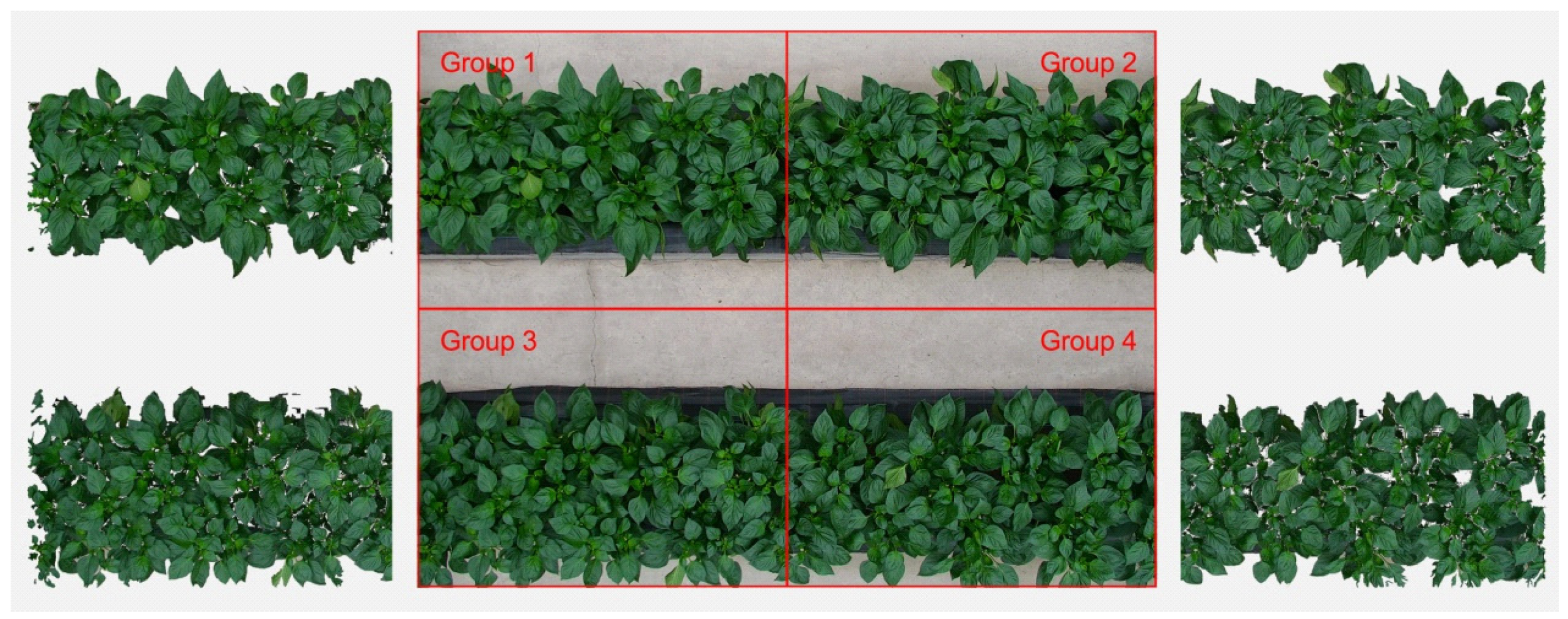
Figure 1.
Image grouping scheme and image separation effect of pepper in the greenhouse.
Figure 1.
Image grouping scheme and image separation effect of pepper in the greenhouse.
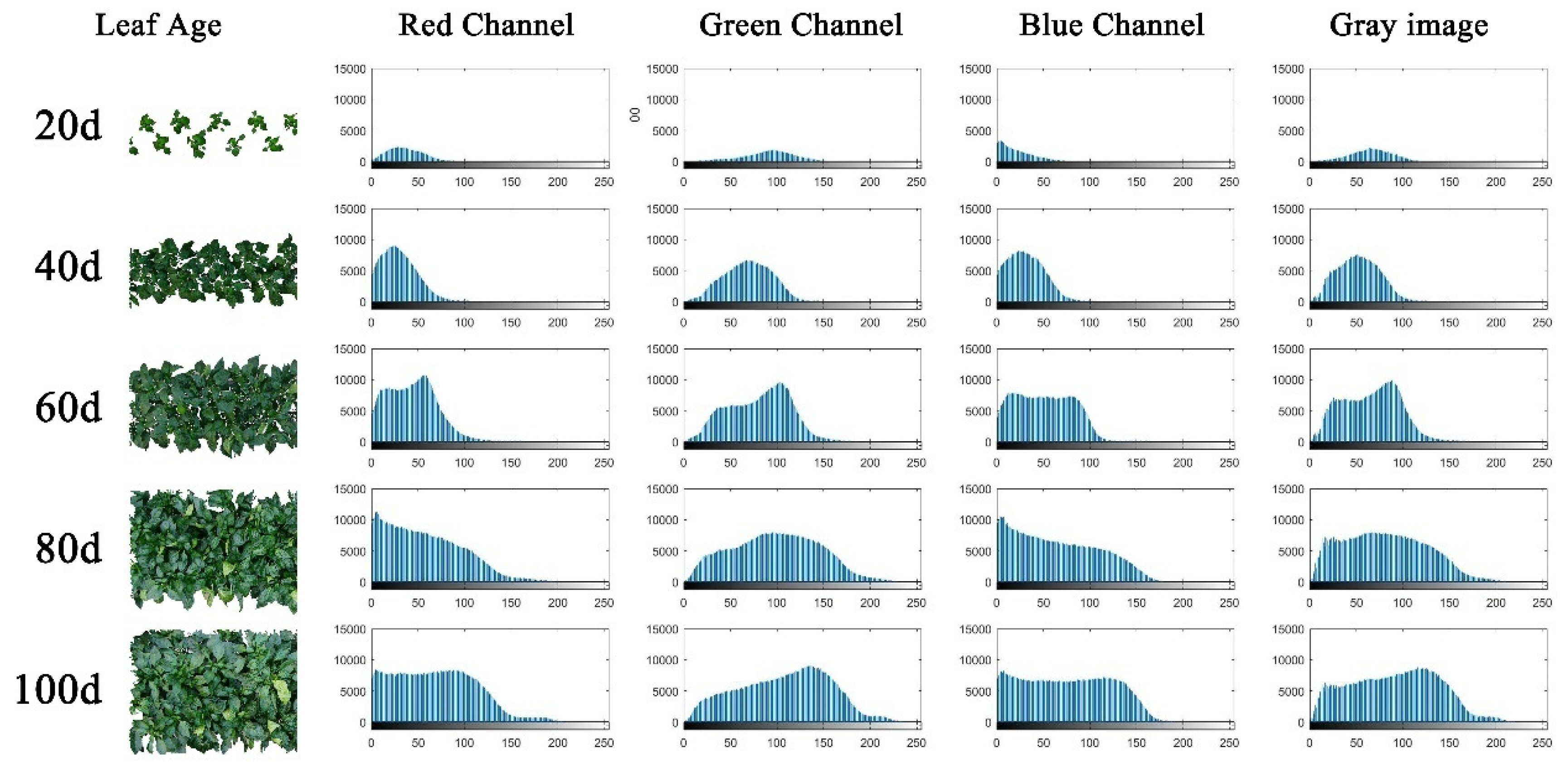
Figure 2.
RGB model color gradation distribution of population canopy images of pepper on five different dates. The cumulative frequency histogram of red, green, and blue channels, as well as gray-level images, were drawn using the imhist function of MATLAB. The X-axis is the color gradation value, and the Y-axis is the cumulative frequency.
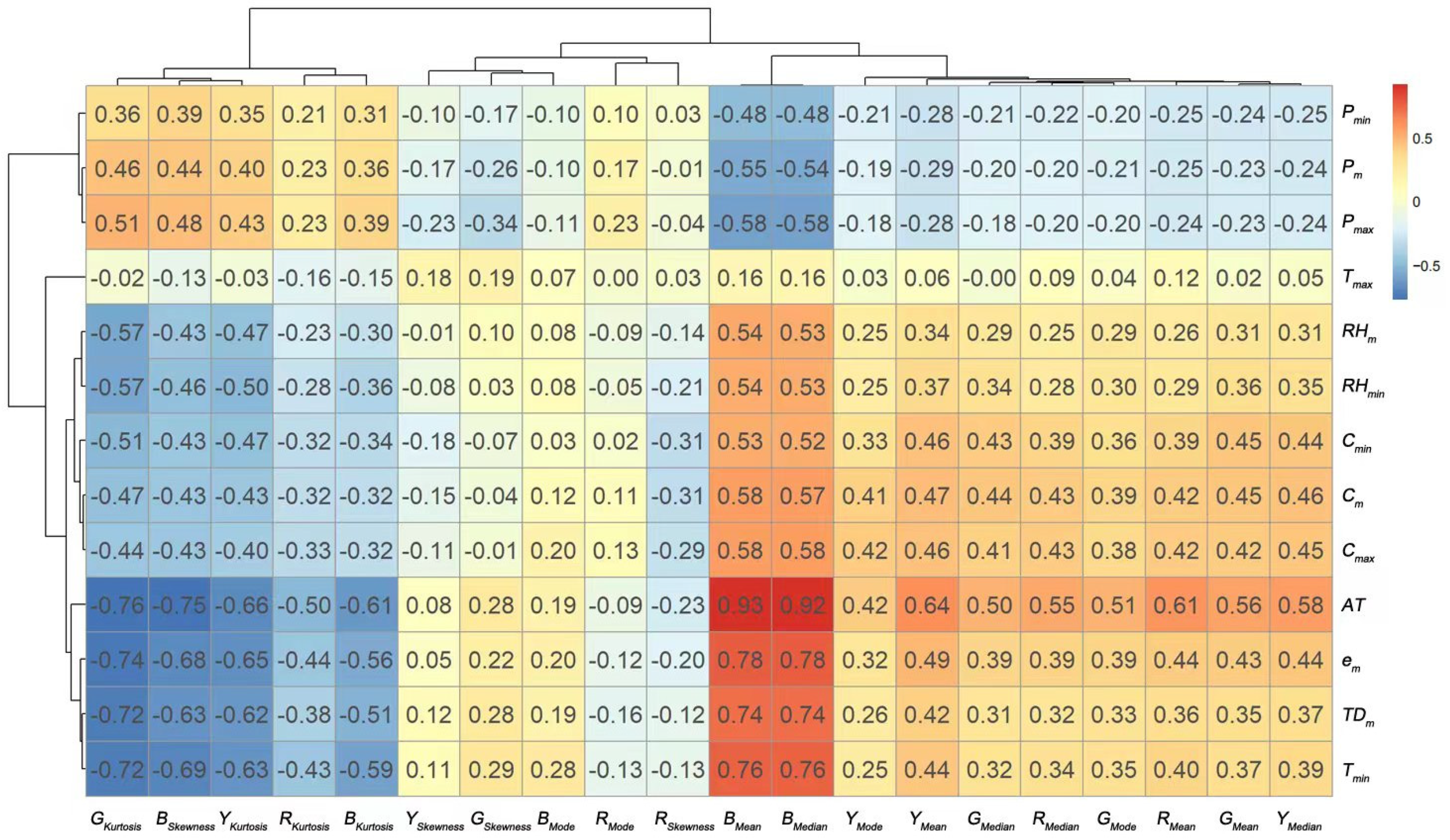
Figure 3.
Spearman correlation coefficient of population canopy CGSD parameters of pepper and microclimate factors. A Spearman correlation analysis of SPSS software was used on 20 CGSD parameters (RMean, RMedian, RMode, RSkewness, RKurtosis, GMean, GMedian, GMode, GSkewness, GKurtosis, BMean, BMedian, BMode, BSkewness, BKurtosis, YMean, YMedian, YMode, YSkewness, and YKurtosis), the microclimate factors, including daily meteorological factors (Tm, Tmax, Tmin, Pm, Pmax, Pmin, RHm, RHmin, TDm, em, Cm, Cmax, Cmin), and accumulation factors (AT) (n = 101). The correlation coefficient obtained by related analysis was drawn to CGSD parameters–daily meteorological factors heat map. The positive correlation coefficient is shown in red, and the negative correlation coefficient is shown in blue.
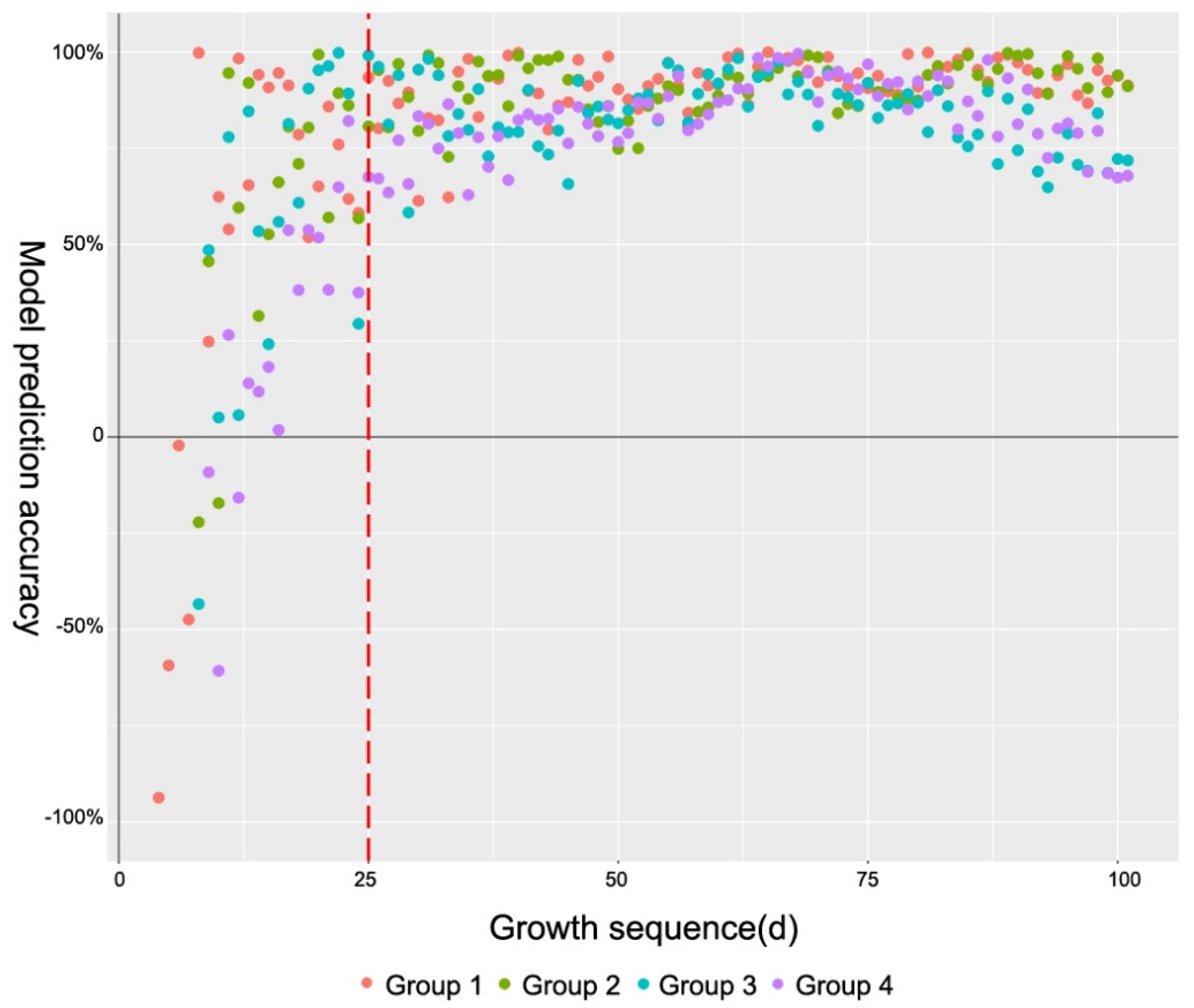
Figure 4.
Scatter plot of inversion accuracy of the inversion models for the samples of four groups. The figure shows only the inversion accuracy values in the interval [−1, 1].
Figure 4.
Scatter plot of inversion accuracy of the inversion models for the samples of four groups. The figure shows only the inversion accuracy values in the interval [−1, 1].
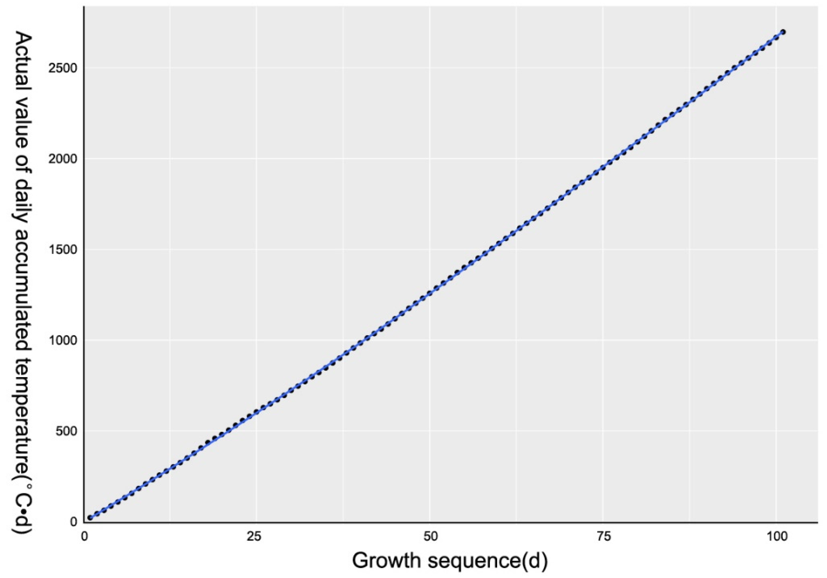
Figure 5.
Scatter plot of daily accumulated temperature during the whole growth period of pepper. GSkewness was fitted by the local polynomial regression-fitting algorithm, which was implemented by the geom_smooth function of R. X axis was the sequence of daily leaf age, and Y axis was the value of the daily accumulated temperature.
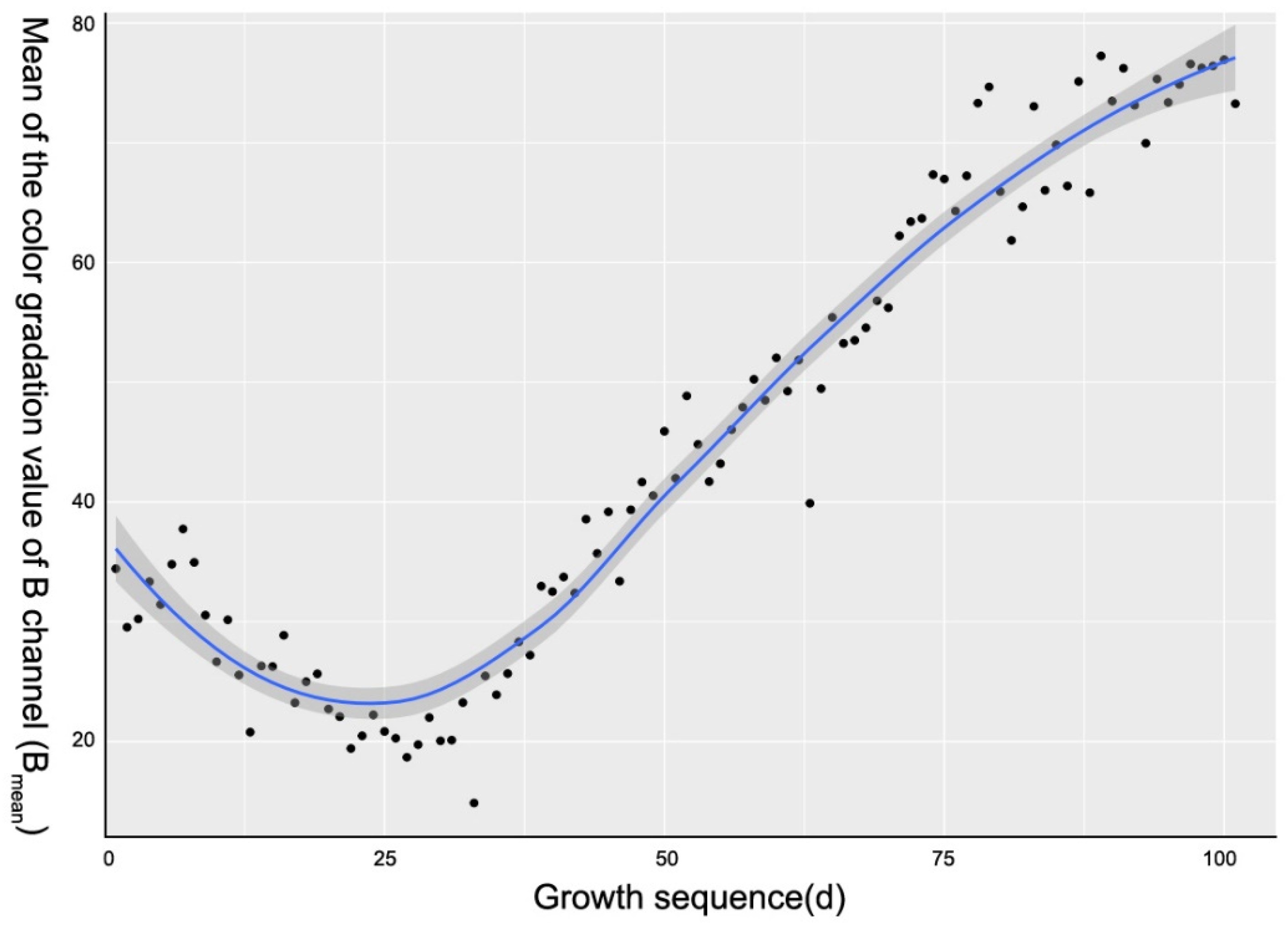
Figure 6.
Scatter plot of BMeans during the whole growth period of pepper. BMean was fitted by the local polynomial regression-fitting algorithm, which was implemented by the geom_smooth function of R. X axis was the sequence of daily leaf age, and Y axis was the daily value of BMean.
Figure 6.
Scatter plot of BMeans during the whole growth period of pepper. BMean was fitted by the local polynomial regression-fitting algorithm, which was implemented by the geom_smooth function of R. X axis was the sequence of daily leaf age, and Y axis was the daily value of BMean.
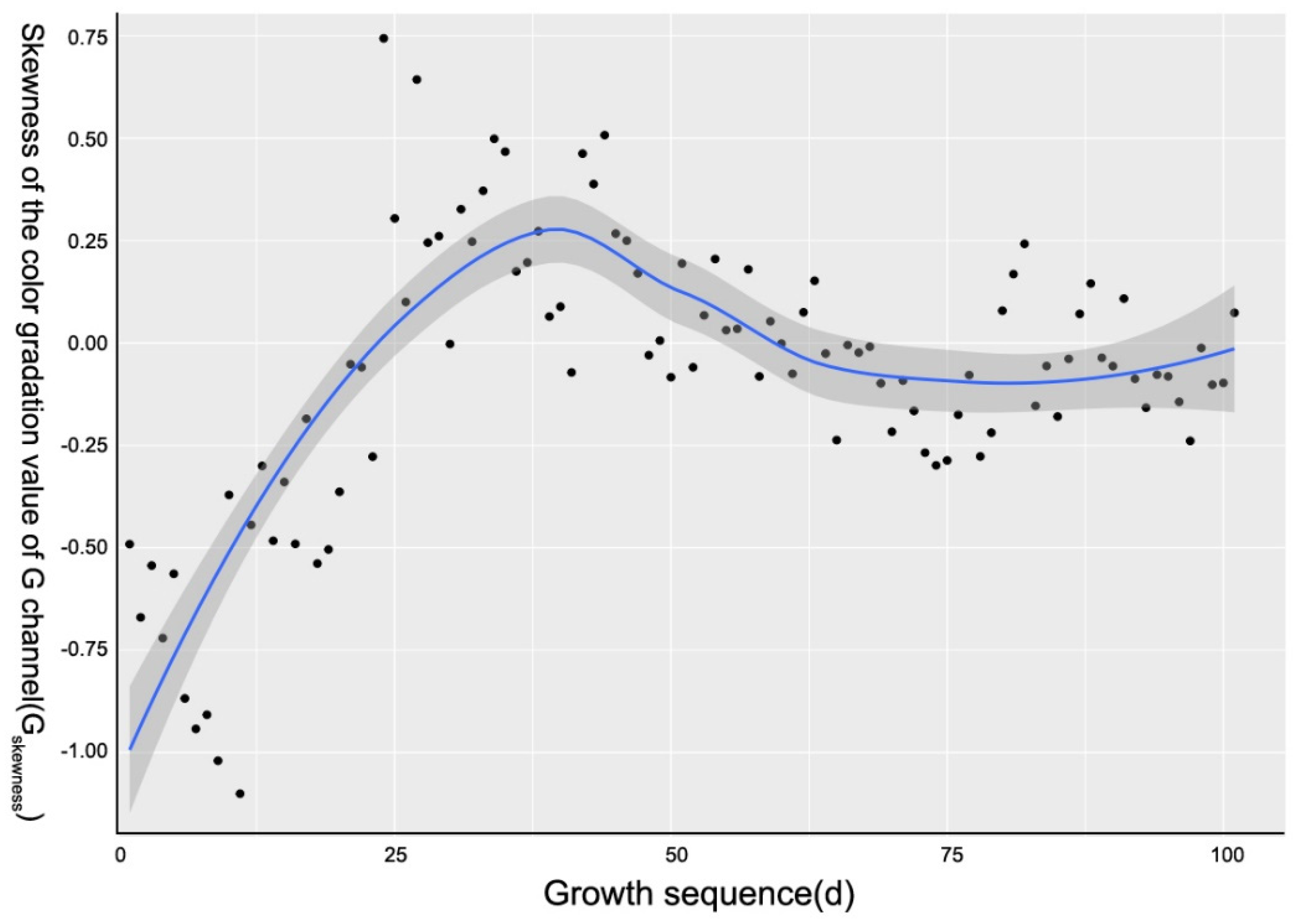
Figure 7.
Scatter plot of GSkewness during the whole growth period of pepper. GSkewness was fitted by the local polynomial regression-fitting algorithm, which was implemented by the geom_smooth function of R. X axis was the sequence of daily leaf age, and Y axis was the daily value of GSkewness.
Figure 7.
Scatter plot of GSkewness during the whole growth period of pepper. GSkewness was fitted by the local polynomial regression-fitting algorithm, which was implemented by the geom_smooth function of R. X axis was the sequence of daily leaf age, and Y axis was the daily value of GSkewness.
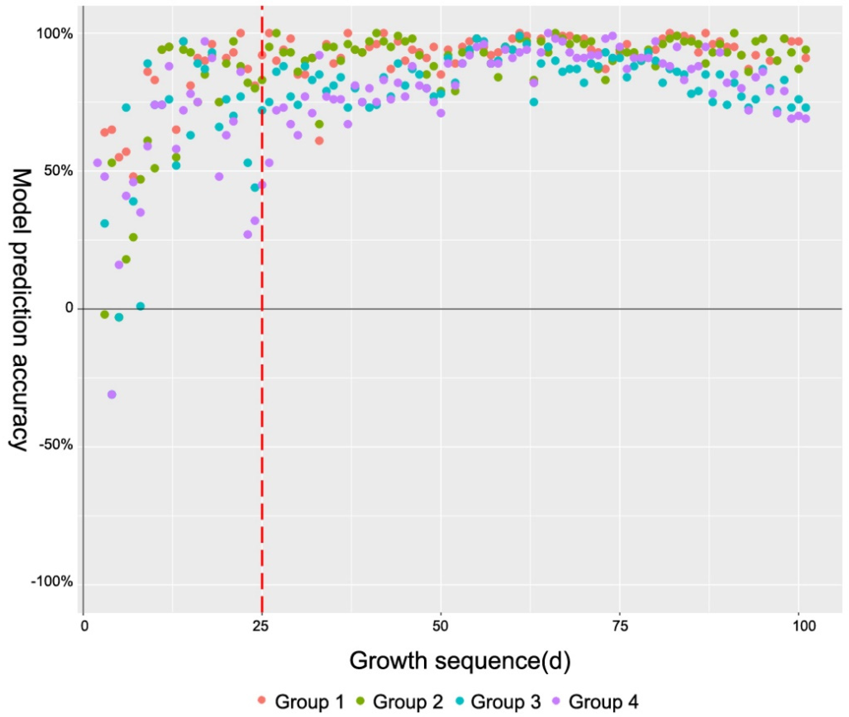
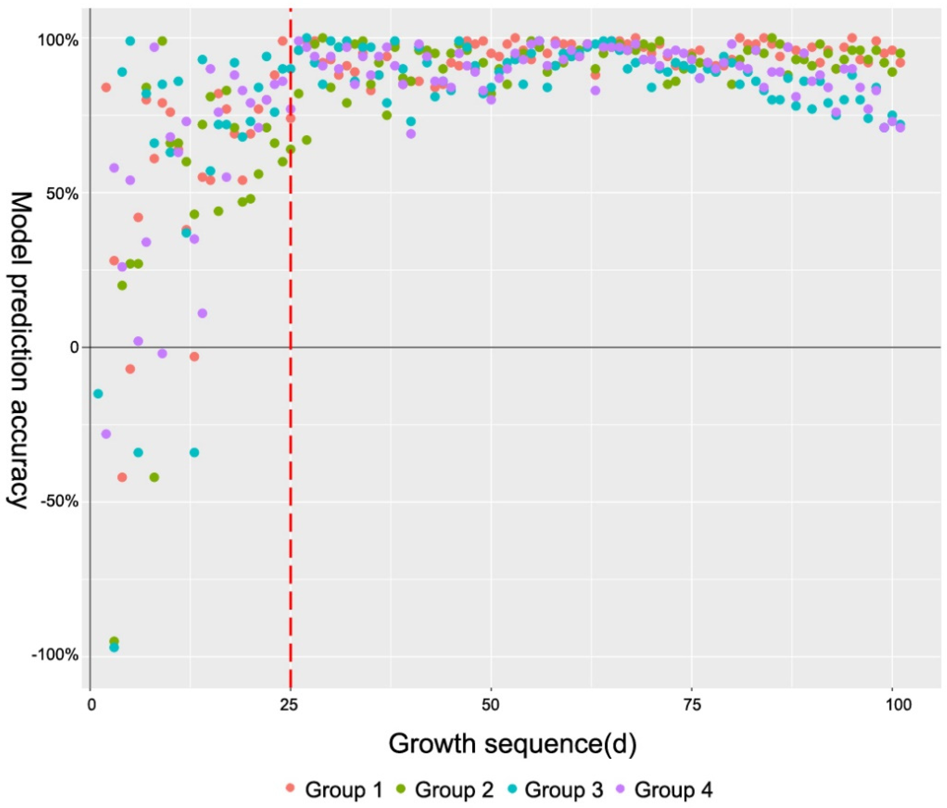
Figure 8.
Scatter plot of inversion accuracy of Y26 for the samples of four groups. The figure shows only the inversion accuracy values in the interval [−1, 1]. The red dotted line in the figure caption is the auxiliary observation line at the 25th day of growth sequence.
Figure 8.
Scatter plot of inversion accuracy of Y26 for the samples of four groups. The figure shows only the inversion accuracy values in the interval [−1, 1]. The red dotted line in the figure caption is the auxiliary observation line at the 25th day of growth sequence.
Figure 9.
Scatter plot of inversion accuracy of Y27 for the samples of four groups. The figure shows only the inversion accuracy values in the interval [−1, 1]. The red dotted line in the figure caption is the auxiliary observation line at the 25th day of growth sequence.
Figure 9.
Scatter plot of inversion accuracy of Y27 for the samples of four groups. The figure shows only the inversion accuracy values in the interval [−1, 1]. The red dotted line in the figure caption is the auxiliary observation line at the 25th day of growth sequence.
Table 1.
Canopy leaf color response regression models of pepper and their goodness of fit.
Table 1.
Canopy leaf color response regression models of pepper and their goodness of fit.
| Models | R-Square | Adjusted R-Square | RMSE | F Value | Significance F |
|---|
| RMean | Y1 = −1137.831 + 0.019 AT + 2.774 Pmax − 1.629 Pmin | 0.508 | 0.493 | 10.672 | 33.374 | 0.000 |
| RMedian | Y2 = −1186.280 + 0.018 AT + 2.960 Pmax − 1.769 Pmin | 0.458 | 0.441 | 11.246 | 27.340 | 0.000 |
| RMode | Y3 = −1054.301 + 2.880 Pmax + 0.016 Cmax − 1.821 Pmin | 0.172 | 0.146 | 17.325 | 6.710 | 0.000 |
| RSkewness | Y4 = −0.174 − 0.002 Cmin + 0.029 RHm − 0.030 em | 0.193 | 0.168 | 0.421 | 7.717 | 0.000 |
| RKurtosis | Y5 = 120.664 − 0.002 AT − 0.113 Pmax | 0.280 | 0.265 | 1.901 | 19.026 | 0.000 |
| GMean | Y6 = −1030.263 + 0.015 AT + 2.477 Pmax − 1.399 Pmin + 0.014 Cm | 0.458 | 0.436 | 10.805 | 20.320 | 0.000 |
| GMedian | Y7 = −1174.908 + 0.015 AT + 2.840 Pmax − 1.620 Pmin + 0.017 Cm | 0.420 | 0.396 | 12.335 | 17.367 | 0.000 |
| GMode | Y8 = −1397.657 + 0.024 AT + 3.486 Pmax − 2.043 Pmin | 0.357 | 0.337 | 18.080 | 17.932 | 0.000 |
| GSkewness | Y9 = 22.809 − 0.069 Pmax + 0.047 Pmin − 0.001 Cmin | 0.264 | 0.241 | 0.299 | 11.601 | 0.000 |
| GKurtosis | Y10 = 22.211 + 0.0004 AT − 0.032 em − 0.018 Pmin | 0.627 | 0.616 | 0.350 | 54.394 | 0.000 |
| BMean | Y11 = −783.168 + 0.025 AT + 0.785 Pmax + 0.007 Cmax | 0.884 | 0.880 | 6.752 | 245.771 | 0.000 |
| BMedian | Y12 = −809.815 + 0.026 AT + 0.807 Pmax + 0.007 Cmax | 0.878 | 0.874 | 7.186 | 232.068 | 0.000 |
| BMode | Y13 = −14.306 + 1.457 Tmin | 0.078 | 0.069 | 17.553 | 8.370 | 0.000 |
| BSkewness | Y14 = 1.500 − 0.001 AT | 0.565 | 0.560 | 0.395 | 128.410 | 0.000 |
| BKurtosis | Y15 = 20.585 − 0.001 AT − 0.539 Tm − 0.005 Cmin | 0.430 | 0.412 | 2.357 | 24.352 | 0.000 |
| YMean | Y16 = −965.515 + 0.018 AT + 2.523 Pmax − 1.525 Pmin | 0.524 | 0.509 | 10.168 | 35.587 | 0.000 |
| YMedian | Y17 = −1099.405 + 0.017 AT + 2.301 Pmax − 1.155 Pmin + 0.032 Cm − 0.384 RHm | 0.522 | 0.497 | 10.981 | 20.775 | 0.000 |
| YMode | Y18 = 74.780 + 0.024 Cmax + 0.017 AT − 2.193 TDm | 0.286 | 0.264 | 19.612 | 12.958 | 0.000 |
| YSkewness | Y19 = 21.832 − 0.063 Pmax − 0.001 Cmin + 0.042 Pmin | 0.212 | 0.187 | 0.341 | 8.692 | 0.000 |
| YKurtosis | Y20 = 5.158 − 0.001 AT − 0.049 em | 0.465 | 0.454 | 0.765 | 42.565 | 0.000 |
Table 2.
Analytical results of inversion accuracy of the inversion model of Y21 for the samples of four groups.
Table 2.
Analytical results of inversion accuracy of the inversion model of Y21 for the samples of four groups.
| Index | Modeling Group (Group 1) | Group 2 from Same Planting Row | Group 3 from Different Planting Row | Group 4 from Different Planting Row |
|---|
| Sample number | 101 | 101 | 101 | 101 |
| Outlier number | 7 | 9 | 8 | 11 |
| Outlier ratio | 6.93% | 8.91% | 7.92% | 10.89% |
| Inversion accuracy | 88.62% | 87.87% | 80.37% | 76.78% |
Table 3.
The univariate quadratic and cubic equation models of Bmean and Gskewness to accumulated temperature.
Table 3.
The univariate quadratic and cubic equation models of Bmean and Gskewness to accumulated temperature.
| Models | R-Square | Adjusted R-Square | RMSE | F Value | Significance F |
|---|
| BMean Y22 = 0.0000070982 AT2 + 0.0038009585 AT + 23.89 | 0.897 | 0.895 | 6.326 | 426.329 | 0.000 |
| BMeanY23 = −0.0000000132 AT 3 + 0.0000604278 AT 2 − 0.0534623558 AT + 36.65 | 0.962 | 0.961 | 3.847 | 824.278 | 0.000 |
| GSkewnessY24 = −0.0000003471 AT 2 + 0.0010537988 AT − 0.65 | 0.391 | 0.378 | 0.270 | 31.433 | 0.000 |
| GSkewnessY25 = 0.0000000004 AT 3 − 0.0000020405 AT 2 + 0.0028721223 AT − 1.05 | 0.604 | 0.592 | 0.219 | 49.345 | 0.000 |
Table 4.
The first derivative equation models of Bmean and Gskewness to accumulated temperature.
Table 4.
The first derivative equation models of Bmean and Gskewness to accumulated temperature.
| Model | First Derivative Equation | x1 | x2 |
|---|
| Y23 | Y23′ = 0.0000000396 AT 2 + 0.0001208546 AT − 0.0534623558 | 536.78 | 2515.14 |
| Y25 | Y25′ = 0.0000000012 AT 2 − 0.0000080810 AT + 0.0028721223 | 994.74 | 2406.09 |
Table 5.
The piecewise inversion model of accumulated temperature to canopy color based on the points of demarcation.
Table 5.
The piecewise inversion model of accumulated temperature to canopy color based on the points of demarcation.
| Models | R-Square | Adjusted R-Square | RMSE | F Value | Significance F |
|---|
| Tt = 1–537 | Y26-1 = 728.655 − 10.377 RMode | 0.849 | 0.841 | 63.410 | 112.130 | 0.000 |
| Tt > 537 | Y26-2 = 33.381 + 33.397 BMean − 3.705 RMode | 0.963 | 0.962 | 123.844 | 991.054 | 0.000 |
| Tt = 1–995 | Y27-1 = 1978.483 − 14.777 GMode − 175.613 BSkewness | 0.849 | 0.841 | 114.955 | 104.333 | 0.000 |
| Tt > 995 | Y27-2 = −790.630 + 43.366 BMean + 562.171 BSkewness − 2.945 RMean | 0.953 | 0.950 | 111.400 | 383.353 | 0.000 |
Table 6.
Comparison of inversion effects of the piecewise inversion models of Y26 and Y27 to Y21.
Table 6.
Comparison of inversion effects of the piecewise inversion models of Y26 and Y27 to Y21.
| | Modeling Group (Group 1) | Group 2 from Same Planting Row | Group 3 from Different Planting Row | Group 4 from Different Planting Row | Summarized Result |
|---|
| Sample number | 101 | 101 | 101 | 101 | 404 |
| Y21 | Outlier number | 7 | 9 | 8 | 11 | 35 |
| Outlier ratio | 6.93% | 8.91% | 7.92% | 10.89% | 8.66% |
| Inversion accuracy | 88.62% | 87.87% | 80.37% | 76.78% | 83.41% |
| Y26 | Outlier number | 2 | 4 | 4 | 2 | 12 |
| Outlier ratio | 1.98% | 3.96% | 3.96% | 1.98% | 2.97% |
| Inversion accuracy | 90.48% | 88.63% | 80.24% | 78.33% | 84.42% |
| Y27 | Outlier number | 4 | 4 | 5 | 3 | 16 |
| Outlier ratio | 3.96% | 3.96% | 4.95% | 2.97% | 3.96% |
| Inversion accuracy | 88.76% | 85.37% | 86.45% | 84.10% | 86.17% |


