
Evaluation of the CAS-ESM2-0 Performance in Simulating the Global Ocean Salinity Change

1
Eco-Environmental Monitoring and Research Center, Pearl River Valley and South China Sea Ecology and Environment Administration, Ministry of Ecology and Environment, PRC, Guangzhou 510611, China
2
International Center for Climate and Environment Sciences, Institute of Atmospheric Physics, Chinese Academy of Sciences, Beijing 100029, China
*
Author to whom correspondence should be addressed.
Atmosphere 2023, 14(1), 107; https://doi.org/10.3390/atmos14010107
Submission received: 8 December 2022
/
Revised: 25 December 2022
/
Accepted: 27 December 2022
/
Published: 3 January 2023
(This article belongs to the Special Issue Climate Change on Ocean Dynamics)
Abstract
:The second version of the Chinese Academy of Sciences Earth System Model, CAS-ESM2-0, is a newcomer that contributes to Coupled Model Intercomparison Project simulations in the community. We evaluated the model’s performance in simulating the salinity for climatology, seasonal cycles, long-term trends, and time series of climatic metrics by comparing it with the ensemble mean of available gridded observations. The results showed that CAS-ESM2-0 could reproduce large-scale patterns of ocean salinity climatology and seasonal variations, despite the fresh biases in the low- and mid-latitudes for climatology, stronger seasonal variation of sea surface salinity within 20° S–20° N, and large uncertainty with the zonal-band structure for 0–1000 m averaged salinity. For long-term changes, the model revealed increased contrast between the salinity of the Atlantic and Pacific basins. However, regional differences in locations and strengths for salinity pattern amplification suggest substantial uncertainty when simulating regional multidecadal salinity changes. The simulated variations in climate metrics for salinity pattern amplification are consistent with the observations and will continue to intensify until the end of this century. Our assessment provides new features of the CAS-ESM2-0 model and supports further studies on model development.
1. Introduction
Ocean salinity is a key variable that drives ocean circulation and modulates the living conditions of marine life, which has implications for global climate and marine ecosystems [1,2]. For example, the Atlantic Meridional Overturning Circulation (AMOC) is maintained and monitored by the temperature and salinity states of the surface waters in the Subpolar North Atlantic Ocean. Additionally, the changes in ocean salinity have been identified as an ideal indicator of the hydrological cycle because it is mainly balanced by the surface freshwater fluxes, such as precipitation, evaporation, river runoff, sea ice melting, and ocean dynamics [3]. Therefore, simulating the ocean salinity accurately is important for monitoring and predicting changes in the climate and Earth systems.
The Coupled Model Intercomparison Project (CMIP) is an important evaluation tool that combines Earth’s climate systems from worldwide institutions with a standard experimental protocol and infrastructure [4]. The latest version is the CMIP6 (Phase 6), which has made substantial improvements in model resolution, computational efficiency, and the representation of physical and biochemical processes [4]. The Chinese Academy of Sciences Earth System Model version 2 (CAS-ESM2-0) was recently launched as a newcomer to the CMIP6 models. It has been developed as an Earth system model to simulate the physical climate system, global environmental processes of air pollution, and carbon cycle [5]. Previous studies have assessed its performance by comparing it with observations and other CMIP5/6 models [5,6,7,8,9]. For instance, the CAS-ESM2-0 model indicates smaller biases than many other CMIP6 models in simulating cloud-radiation forcing and tropical precipitation, which contributes to the largest modeling uncertainty [10]. The advantages of the CAS-ESM2-0 ocean component in simulating the horizontal heat transport, sea surface height, and AMOC vertical structure have been demonstrated [11,12]. The El Niño-Southern Oscillation (ENSO) is one of the most important interannual variabilities in the Earth’s climate system [13]. While the CAS-ESM2-0 model is at the forefront of the CMIP6 members in its simulation and prediction [14], it still shows a stronger amplitude of the simulated ENSO [5]. Several essential variables have been systematically examined in previous studies, including precipitation, sea ice, East Asian summer monsoon, SST, and so on. However, few studies have assessed the performance of the CAS-ESM2-0 model in simulating ocean salinity change. They did not fully consider its capability to stimulate the different temporal and spatial salinity variabilities and predict the salinity response in future climate change. However, the model performance of ocean salinity exerts an important influence on the ocean dynamics and the accuracy of climate predictions [15]. For instance, the salinity change is closely related to the ENSO, Indian Ocean Dipole (IOD), and other climate variabilities by modulating the upper ocean circulation [16,17,18,19]. The prediction of ENSO based on the close relationship between mixed-layer salinity (MLS) tendency and Niño3.4 index tends to be less effective due to the salinity biases [20]. Thus, it is the starting point of our analysis.
This study aims to evaluate the ability of the CAS-ESM2-0 model to simulate ocean salinity variability over the near-historical period (1960–2014) and twenty-first-century projection period (2015–2100) under the strongest future climate scenarios by assessing its performance using several temporal and spatial variabilities, including climatology, seasonal cycles, long-term linear trends, time series of climate index, and future patterns in salinity. The remainder of this paper is organized as follows. Section 2 describes the data and methods used in this study. Section 3 presents the results of the simulated performance, and Section 4 summarizes the findings.
2. Materials and Methods
2.1. CAS-ESM2-0
The CAS-ESM2-0 model is a fully coupled earth system model produced by the Institute of Atmospheric Physics, Chinese Academy of Sciences (IAP, CAS). Compared with the previous version of CAS-ESM1-0 released in 2015, the CAS-ESM2-0 model has improved codes and parameterization schemes for most components and new schemes for atmospheric convection and clouds [6]. It has five main climate components of the atmosphere, ocean, land, and sea ice, including the fifth generation of the IAP Atmospheric General Circulation Model, Climate System Ocean Model version 2 [21], Los Alamos Sea-Ice model version 4 [22], Beijing Normal University/IAP Common Land Model [23], and Weather Research and Forecast Model [24]. These components were coupled by model coupler 7 through the infrastructure of the Community Earth System Model. Other components included IAP dynamic vegetation, fire, and ocean biogeochemistry models.
Here, we evaluated the performance of ocean salinity for the CAS-ESM2-0 historical simulation over 1960–2014, as well as the ScenarioMIP concentration-driven simulations of the 21st century (2015–2100) according to the strongest forcing trajectory in the Shared Socioeconomic Pathways (SSP5-8.5). They were performed in line with the CMIP6 reference protocols [4,25], which are obtained from the Earth System Grid Federation (ESGF) archives (https://esgf-node.llnl.gov/search/cmip6, assessed on 1 September 2022). The absolute salinity was used in the study with the unit of g kg−1.
2.2. Observations
We used four observational datasets to evaluate the performance of the CAS-ESM2-0 models by comparing the different salinity variabilities with their ensemble mean. The salinity datasets include Institute of Atmospheric Physics (IAP) data [26], EN4 from the Met Office Hadley Centre [27], National Centers for Environmental Information (NCEI) data [28,29], and Ishii from the Japan Meteorological Agency [30]. These data were objectively analyzed based only on salinity observations and had the same 1° × 1° horizontal resolution, spanning from 1960 to 2020. The IAP, EN4, and Ishii data provided monthly gridded analyses, and the NCEI data were calculated from the 5-year smoothing mean. The key advantage of the analyzed data is the application of an advanced and systematically evaluated mapping scheme to fill the data gaps based on the sparse salinity observations. These datasets adopt different mapping methods, and their ensemble mean helps hidden errors to obtain the robust signal in observations. For a fair comparison, they have also been interpolated into 41 levels at depths of 0–2000 m vertically, which is the same as the IAP data. The calculation of the ensemble mean from these datasets provided an advanced and careful evaluation of CAS-ESM2-0 performance.
For the ocean components, the CAS-ESM2-0 model had a nominal resolution of 1° with a finer meridional spacing near the equator. To facilitate intercomparison and validation against the observations, the CAS-ESM2-0 model was also spatially remapped to a horizontal resolution of 1° × 1° using bilinear interpolation and 41 vertical levels at depths of 0–2000 m, consistent with the resolutions of the IAP gridded dataset. The mean state was calculated by the annual mean within the 1990–2010 baseline, and the seasonal variation was averaged by the 12-month climatological mean from 1990 to 2010. The monthly salinity anomaly was obtained by removing the climatological means. An ordinary least squares linear regression was used to calculate the linear trends, with the error bar (1-sigma confidence level) accounting for the reduction in the degrees of freedom due to the temporal correlation of the residuals based on the autoregressive moving average model [31]. For the uncertainty level of the linear trends, the 95% confidence interval was presented throughout this study. For the projection analysis, the period of 2020–2040 was adopted as the near-term future and 2080–2100 as the long-term future to investigate the future changes in ocean salinity under different periods of human-forced climate change.
3. Results
3.1. Mean State
3.1.1. Spatial Distribution
Figure 1 shows the spatial distribution of the annual mean sea surface salinity (SSS) and 0–2000 m averaged salinity (S2000) for the observations and CAS-ESM2-0 model. A basin-scale consistency of salinity patterns is located between CAS-ESM2-0 and the observations, with a high spatial correlation coefficient of 0.92 for SSS fields (Figure 1a,c) and 0.86 for S2000 fields (Figure 1b,d). The pattern correlation of SSS fields is larger than other CMIP6 members (mostly between 0.912–0.917) and CMIP5 models (mostly < 0.9) [32], indicating its better performance for CAS-ESM2-0 in SSS simulation. For the SSS fields, the subtropical oceans in all three basins exhibit high values of salinity (>35 g kg–1), and the fresh pools are mainly located in the tropical and subpolar oceans, with a low value of salinity (<34 g kg–1) in the eastern and western regions in the tropical Pacific, North Pacific, and Arctic Ocean. The large-scale SSS pattern shows a high resemblance to the distribution of freshwater flux (evaporation minus precipitation) on the sea surface as the oceanic tracker of the global hydrological cycle [26,33]. For S2000, the salinity distribution is responsible for the combination of surface freshwater forcing and ocean dynamics [26]. The salinity contrast between the salty Atlantic Ocean and the fresher Pacific and Indian Ocean is also apparent in the CAS-ESM2-0 model.
Figure 1e,f also demonstrates the differences between the model and observations for SSS and S2000, respectively, identifying the model biases in the CAS-ESM2-0. For the SSS (Figure 1e), the fresh bias for CAS-ESM2-0 is found in most parts of the global ocean, and strong negative values (<−0.5 g kg–1) are mainly located in the Southern Hemisphere and North Indian Ocean. The Pacific Ocean demonstrates large fresh errors in the subtropical south and east (<−1 g kg–1), with an overall small positive bias in the subtropical south and along the equator to the central Pacific, corresponding to the pattern of the precipitation bias for CAS-ESM2-0 [5]. The excessive wet bias of simulated precipitation on both sides of the drier equatorial Pacific can be attributed to the double Intertropical Convergence Zone (ITCZ) bias for CAS-ESM2-0, which is apparent in climate models but has been improved from the previous version of the CAS-ESM model [5,34]. Ref [5] also shows a large positive precipitation bias in the Southwest Pacific (20° S–30° S), locally different from the smaller negative SSS bias. This implies the modification of ocean transport from fresher waters in the tropics.
In the Indian Ocean, the dipole pattern of the SSS with the saltier water in the Arabian Sea (AS) and fresher in the Bay of Bengal (BoB) was expressed in both the model and observations. The opposite signals are due to the different dominance of atmospheric processes (rainfall or evaporation) and oceanic transport of saltier/fresher water [35]. The CAS-ESM2-0 model shows fresh biases in the whole of the North Indian Ocean and stronger errors in the BoB, which is different from the fresh (salty) bias in the AS (BoB) shown in the ensemble mean of CMIP5 and CMIP6 models [32], and the basin-scale positive salinity bias over the northern BoB and south eastern AS (SEAS)presented in the Coordinated Ocean-ice Reference Experiments interannual protocol (CORE-II) [36]. The magnitude of fresh bias in the North Indian Ocean (<−1 g kg–1) is also stronger than previous estimates in other simulations [37,38]. This weaker zonal contrast of the SSS is generally consistent with the precipitation bias distribution [5]. The freshening in AS and BoB may be attributed to the weaker wind and shortwave radiation forcings in the model simulations [38]. The Atlantic Ocean shows a large portion of fresh bias except in the North of the Gulf of Mexico and its extensions, similar to the results of other CMIP6 models [32].
For the S2000 bias (Figure 1f), the fresh bias of CAS-ESM2-0 with the global mean of –0.056 g kg–1 is more spatially consistent in the Indian and Pacific Oceans, indicating an overall negative bias in the subsurface layer. The largest negative bias of CAS-ESM2-0 (<−0.3 g kg–1) occurs in the North Indian Ocean, leading to unidentified salty regions for observations (Figure 1b). This implies the persistence of a large fresh bias in the subsurface ocean. The Atlantic Ocean and Southern Ocean show an overall salty bias, particularly in the subpolar North Atlantic and tropical Atlantic, different from the SSS biases (Figure 1e) and precipitation bias [5], indicating that ocean dynamics such as AMOC play a more important role.
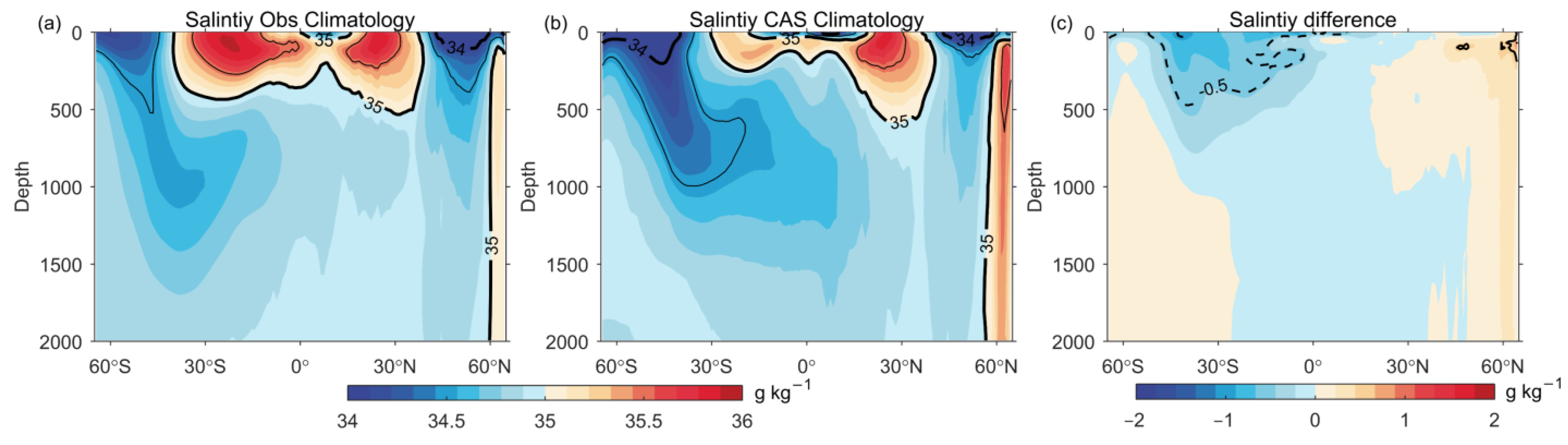
3.1.2. Zonal Mean
Figure 2 illustrates the pattern of global zonal-mean salinity from the surface to 2000 m to evaluate its performance in simulating subsurface change. The observational mean shows a high-salinity bowl extending to the upper 400 m within 30° S–30° N, caused by salty surface water and its subduction in subtropical gyre regions. The observed low-salinity intermediate waters extend to 1000 m and are originated from high latitudes [39]. The CAS-ESM2-0 model reproduces the large-scale salinity distribution in the vertical structure consistent with the observations but with differences in strength and location (Figure 2b). Compared with the observations, the high-salinity bowl in the mid-latitudes is fresher and shallower in the Southern Hemisphere, and the subducted low-salinity waters in the Southern Ocean are much stronger. The model bias for freshwater extends to 500 m in the mid and low latitudes, particularly in the Southern Hemisphere (<−0.5 g kg−1). This implies stronger ventilation of fresher waters in the CAS-ESM2-0 model.
Meanwhile, the CAS-ESM2-0 model shows a better illustration of the subsurface salinity in the Northern hemisphere than other CMIP6 models because it does not show the common fresh bias extending to 350 m [32]. A positive bias also occurs north of 40° N, extending to 2000 m. This may have been induced by the weaker freshwater in the North Pacific and subpolar North Atlantic Ocean and the greater injection of salty Mediterranean water below 100 m in the models. Moreover, the tropical fresh pool is broader and stronger in CAS-ESM2-0 than in the observations (Figure 2a,b), corresponding to the higher rainfall biases outside the equator associated with the double ITCZ bias [5].
3.2. Seasonal Variation
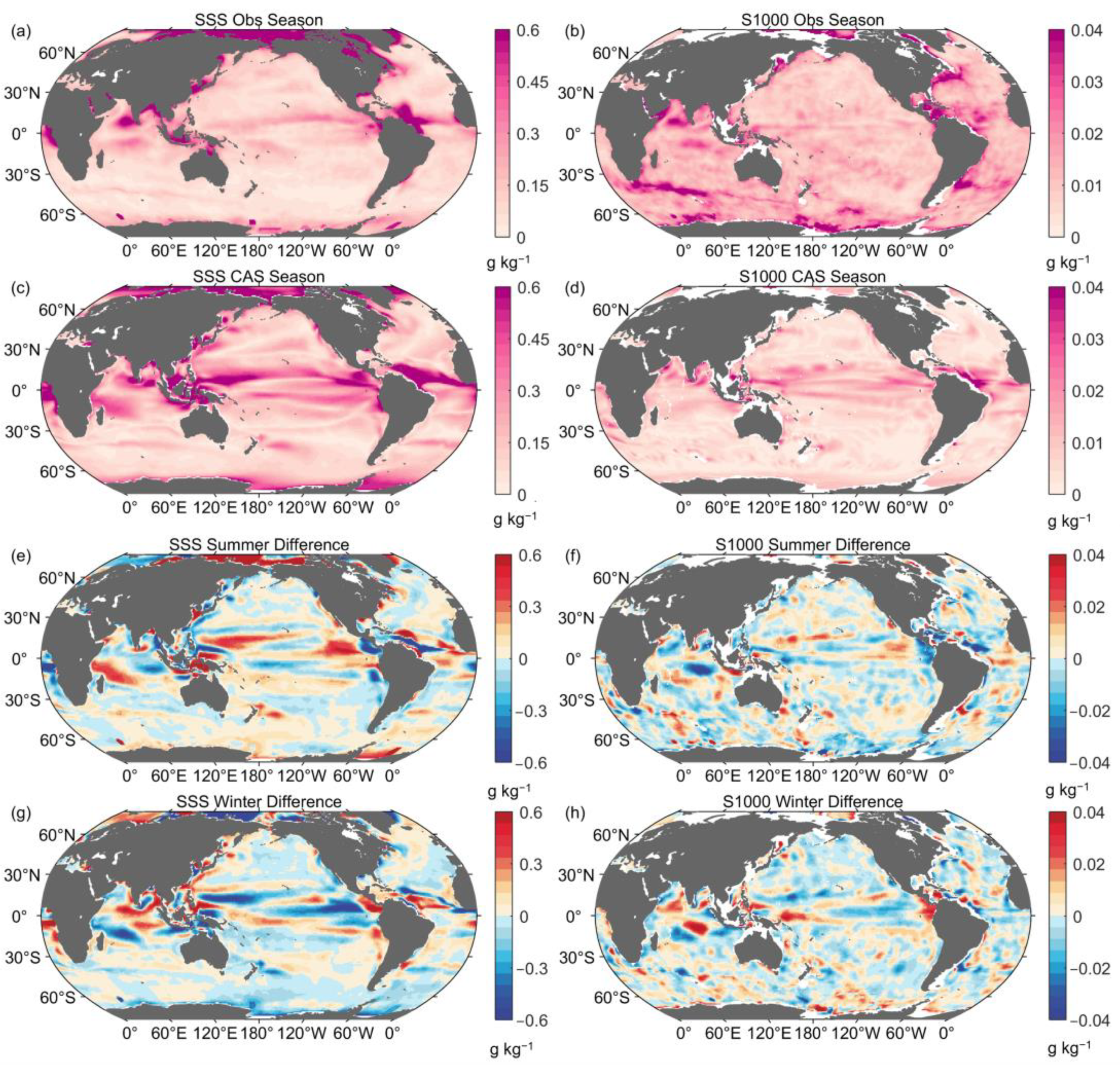
Following the study of [32], we evaluated the seasonal variations in global zonal means of SSS and 0–1000 m averaged salinity (S1000) for the CAS-ESM2-0 model performance (Figure 3). For the observations (Figure 3a), the tropical SSS within 5° N–20° N (20° S–5° N) increases (decreases) in the first half year and tends to be fresher (saltier) in the second half year. This opposing change in the SSS is linked to the seasonal shift in the ITCZ [40]. The mid- and high-latitudes (outside of 30° N/S) also show significant seasonal variations, with the strongest magnitude occurring north of 60° N (>0.8 g kg−1). The CAS-ESM2-0 model shows a seasonal cycle of the SSS similar to the observations but with differences in magnitude (Figure 3a,c). For instance, the magnitude of the seasonal cycle within 20° S–20° N and south of 60° S is stronger than the observational results with more than 0.1 g kg−1 (Figure 3e). The SSS seasonal variation north of 60° N tends to be weaker than that in observations (>0.2 g kg−1). The CAS-ESM2-0 shows a similar seasonal evolution with the ensemble mean of other CMIP6 models, but the magnitude of its variation seems to be stronger [32].
The seasonal variations in observational S1000 also show strong magnitude in polar oceans of both hemispheres (Figure 3b), and their distributions are similar to those in SSS (Figure 3a). The CAS-ESM2-0 shows a good large-scale pattern consistent with the observations, such as the shift from the positive phase in the first half-year to the negative phase in the second half-year within 65° N–80° N and a transfer from the positive phase (April to September) to the negative phase (October to March) within 5° N–20° N. The opposite seasonal variations of SSS in the tropics are diminished by an average of 0–1000 m, implying modulations in ocean dynamics. The S1000 bias indicates many zonal bands and fine structures, and it reaches a similar magnitude for both the model and observations (Figure 3f). The largest errors are found in the polar regions, associated with limited observations of the polar subsurface ocean. These results provide low confidence in assessing the seasonal variation of subsurface salinity for the CAS-ESM2-0 model, particularly at high latitudes.
Figure 4 further denotes the spatial distributions of the magnitude of seasonal variation of SSS and S1000 to indicate the strength of seasonal salinity change. The SSS observations show the high magnitude of the seasonal cycle in ITCZ regions, the Arctic Ocean, and some coastal regions, such as the Gulf of Mexico and its extensions and the tropical western Atlantic. Although the patterns of CAS-ESM2-0 indicate a good similarity with observations, the model displays a stronger magnitude in the tropical ocean (>0.4 g kg−1), corresponding to the large positive (negative) errors in the summer (winter) season (Figure 4e,g). This symmetric distribution of the SSS bias banded along the equator may be due to the double ITCZ bias in models [41]. In the Indian Ocean, the contrasting salinity pattern in the AS and BoB has been detected in previous studies, which is controlled by the combination of surface freshwater forcings, river runoff, and other ocean processes [15,36,40]. The magnitude of variation in the CAS-ESM2-0 model is similar to that in the observations (Figure 4a), but the largest errors are found in winter, with the positive bias in SEAS and negative bias in southern BoB (Figure 4g). For the S1000, the CAS-ESM2-0 model shows a larger magnitude of variation (>0.02 g kg−1) in the tropical Pacific (Figure 4d), than that in observations (Figure 4b). This bias is also found in other CMIP6 models, which is probably linked to the stronger simulated rainfall and its penetration into the subsurface ocean [32,42]. Compared with the observations, the weaker magnitude of variation in the CAS-ESM2-0 model is found in the North Indian Ocean, Antarctic Circumpolar Current (ACC) regions, and the West Atlantic Ocean (Figure 4f). The mean differences in winter and summer seasons show an overall opposite pattern in the global ocean, and the largest errors are mostly located in the tropical Pacific and Indian Oceans. There are some patchy or spotty distributions in the seasonal differences, which is likely due to the large uncertainty in observations [27,29].
3.3. Long-Term Linear Trends over the Past Decades
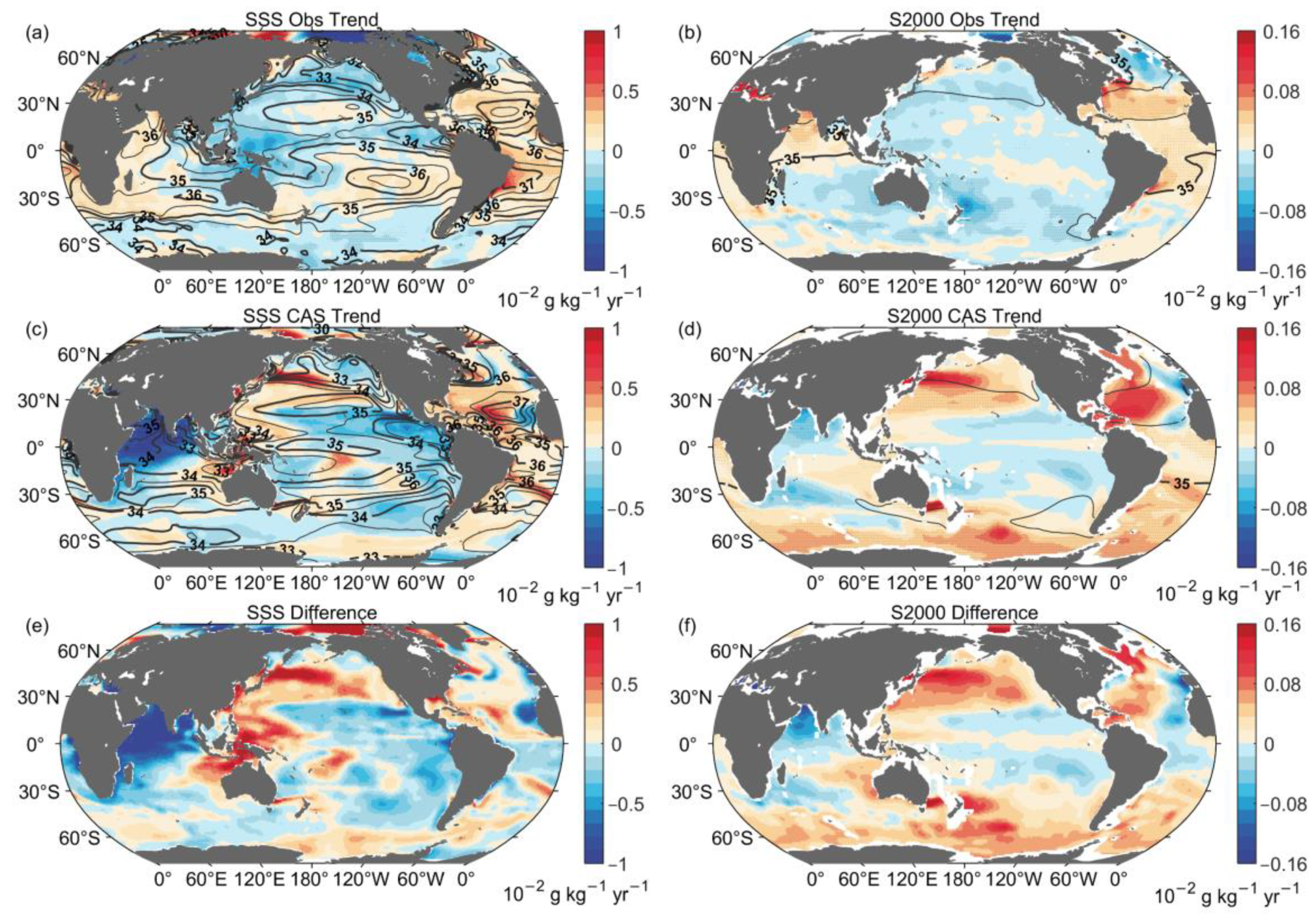
Long-term linear trends in surface and subsurface salinity are well-indicated for the intensification of the global water cycle [26,35]. Here, we investigated the geographic distribution of the linear trends in SSS and S2000 during 1960–2020, as shown in Figure 5. For the SSS change, the observations show an amplified pattern of SSS climatology with saltier (fresher) water in already salty (fresh) regions. The notable features include the salinity increase in the subtropical gyre, the West Indian Ocean, and the Atlantic Ocean, and freshening in the tropical western and eastern Pacific and North Pacific. As indicated in Figure 5c, the CAS-ESM2-0 model reveals the increased salinity contrast between the saltier Atlantic and fresher Pacific Ocean, similar to observations owing to the intensified inter-ocean transport of water vapor [43,44]. However, the model shows a much stronger freshening in the Indian Ocean and much larger salinity increases in the West and Northwest Pacific than in observations. Compared with the CMIP6 multi-model mean of SSS trends over the 1950–2019 period, the CAS-ESM2-0 model shows a good similarity for the large-scale pattern and magnitude, although it shows a stronger freshening in the whole North Indian Ocean and a weaker salinity increase in the subtropical South Pacific [42].
The S2000 for both the model and observations also indicates an increased salinity contrast between the two basins (Figure 5b,d). The observational S2000 increase (decrease) in the North Indian (North Pacific) Ocean is seen where the salinity climatology is high (low) (Figure 5b), while the model shows a different change in these regions. The Atlantic Ocean indicates observational freshening of salinity in the subpolar North Atlantic Ocean, with positive trends elsewhere. However, for CAS-ESM2-0, a broader and stronger salinity increase is found in most regions of the Atlantic Ocean, associated with a greater simulated AMOC transport than the observational estimates [41]. Moreover, the Southern Ocean (south of 40° S) in the CAS-ESM2-0 model is apparent with a larger and broader increasing salinity trend than that in the observations.
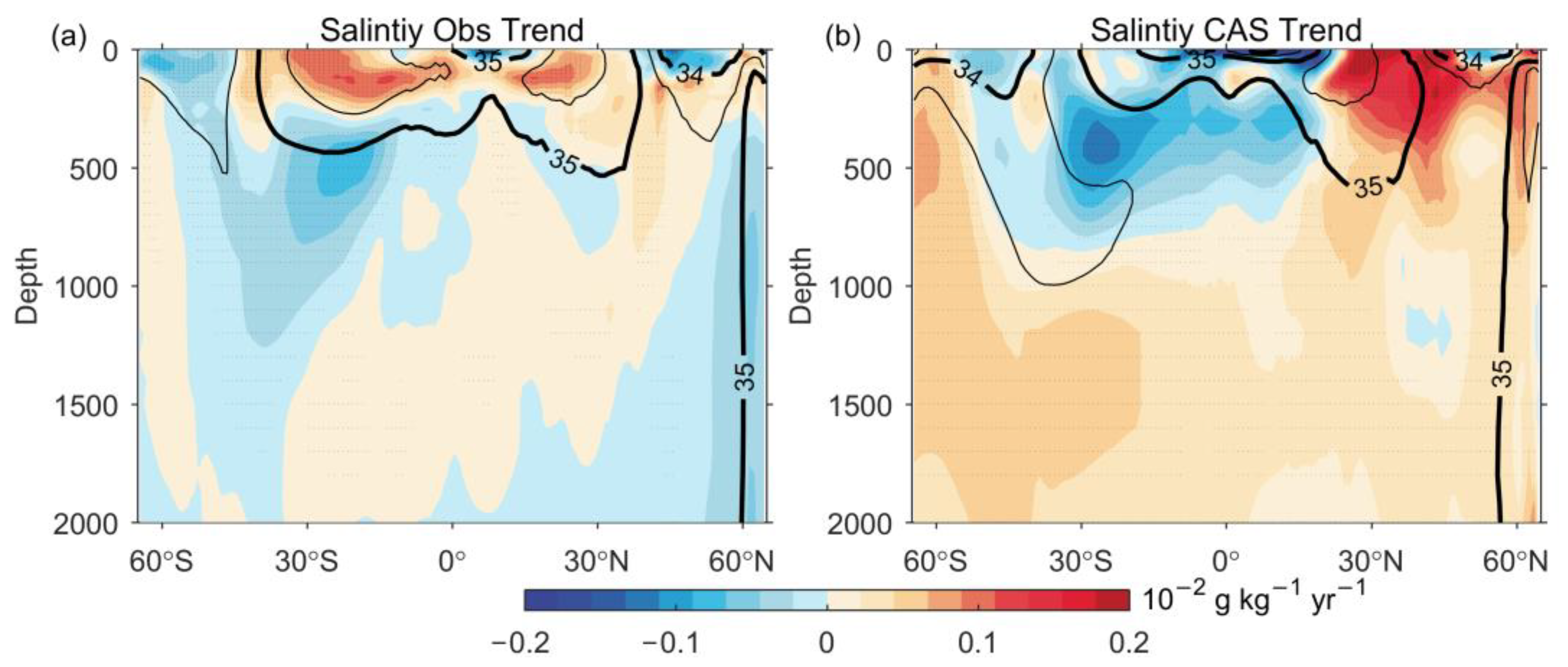
A comparison of linear trends in the global zonal mean of salinity over 1960–2020 between the models and observations is also illustrated in Figure 6. As indicated in the observations, the linear trends in salinity also show the amplification of the mean salinity pattern, with the high-salinity bowl in the upper 300 m within 35° S–30° N and the freshening of low-salinity intermediate waters along the subducted pathway towards 30° N within 500–1000 m (Figure 6a). The CAS-ESM2-0 pattern is similar to large-scale salinity trends, but they also have remarkable differences. For instance, simulated freshening in tropical oceans is broader and deeper than observations. The largest increase in salinity in the Northern Hemisphere is further north, and the southern hemisphere does not exhibit an increase in salinity within the subtropical regions. The surface salinity in the Pacific Ocean shows an overall increasing trend south of 60° S (Figure 5c), inducing different salinity increases in the intermediate layer (below 700 m, Figure 6b), drastically different from the results of the observations (Figure 6a).
3.4. Salinity Contrast Metrics
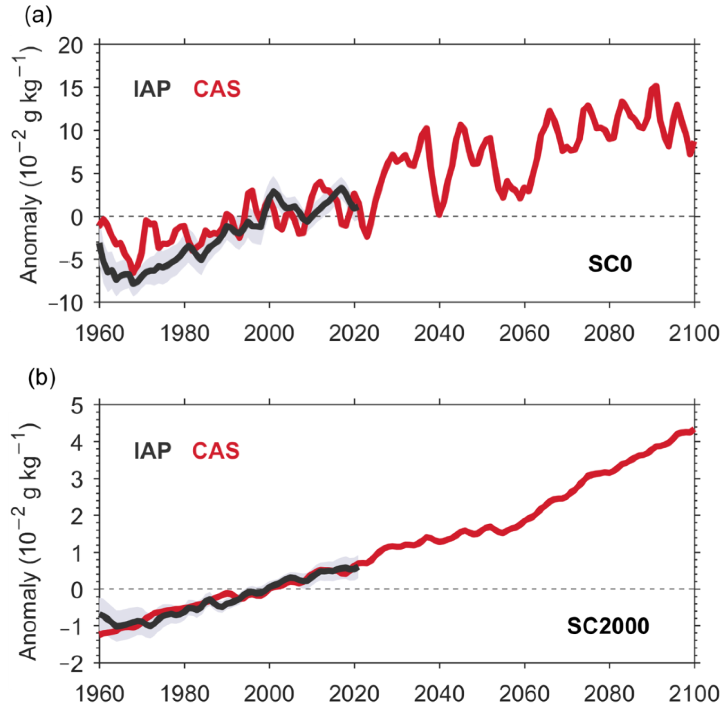
Salinity contrast metrics have been proposed to estimate the amplification of the salinity pattern [26,45], which is calculated by the monthly difference between the salinity average over high- and low-salinity regions. The SSS-contrast (SC0) and S2000-contrast (SC2000) indices were calculated for any ocean volume over the sea surface and 0–2000 m depth, respectively. These metrics allowed us to better indicate and quantify changes in the global hydrological cycle. Here the long-term evolutions of salinity contrast metrics were examined by using the IAP data, which has been proven to provide more accurate quantifications of the salinity pattern amplification [26]. Figure 7 illustrates the global annual mean SC0 and SC2000 anomalies with respect to the 1990–2010 period. The observed SC0 and SC2000 increased substantially from 1960 to 2020, with large trends of 0.179 ± 0.033 g kg–1 century−1 and 0.029 ± 0.004 g kg−1 century−1, respectively. The salinity variations of the CAS-ESM2-0 simulation compared satisfactory with the observational results, with a highly significant linear trend of 0.091 ± 0.005 g kg−1 century−1 for SC0 and 0.030 ± 0.0003 g kg−1 century−1 for SC2000 over the 1960–2020 period, respectively. The simulated SC0 variations corresponded to a lower rate than that of observations, possibly because the negative values of CAS-ESM2-0 were slightly smaller before 1980. The mean difference of SC0 during 1960–1980 between the CAS-ESM2-0 simulation and observations is 0.035 g kg−1. For the SC2000 variation, the CAS-ESM2-0 model has a high correlation coefficient of 0.94 with the observations over the 1960–2010 period. Future projections indicate a steady amplification of the mean salinity pattern under the SSP5-8.5 pathway throughout the 21st century. The projected CAS-ESM2-0 results show an increasing trend of 0.113 ± 0.006 g kg−1 century−1 for SC0 and 0.046 ± 0.001 g kg−1 century−1 for SC2000 within 2020–2100, respectively. The SSS pattern amplification is stronger than the SC2000 changes and demonstrates more rapid fluctuations attributed to the atmospheric forcing and transient response near the surface [46]. Compared with the simulated trends during 1960–2020, the projected trends for SC0 and SC2000 have increased by 24% and 53%, respectively. As an integrated subsurface metric, the SC2000 shows a more robust increase because it is less impacted by the short-term fluctuation of ocean salinity, such as interannual variability [26]. These results indicate that the CAS-ESM2-0 model can reproduce the hydrological cycle amplification during the historical period and portends the persistent intensification of the water cycle under anthropogenic warming.
3.5. Projection
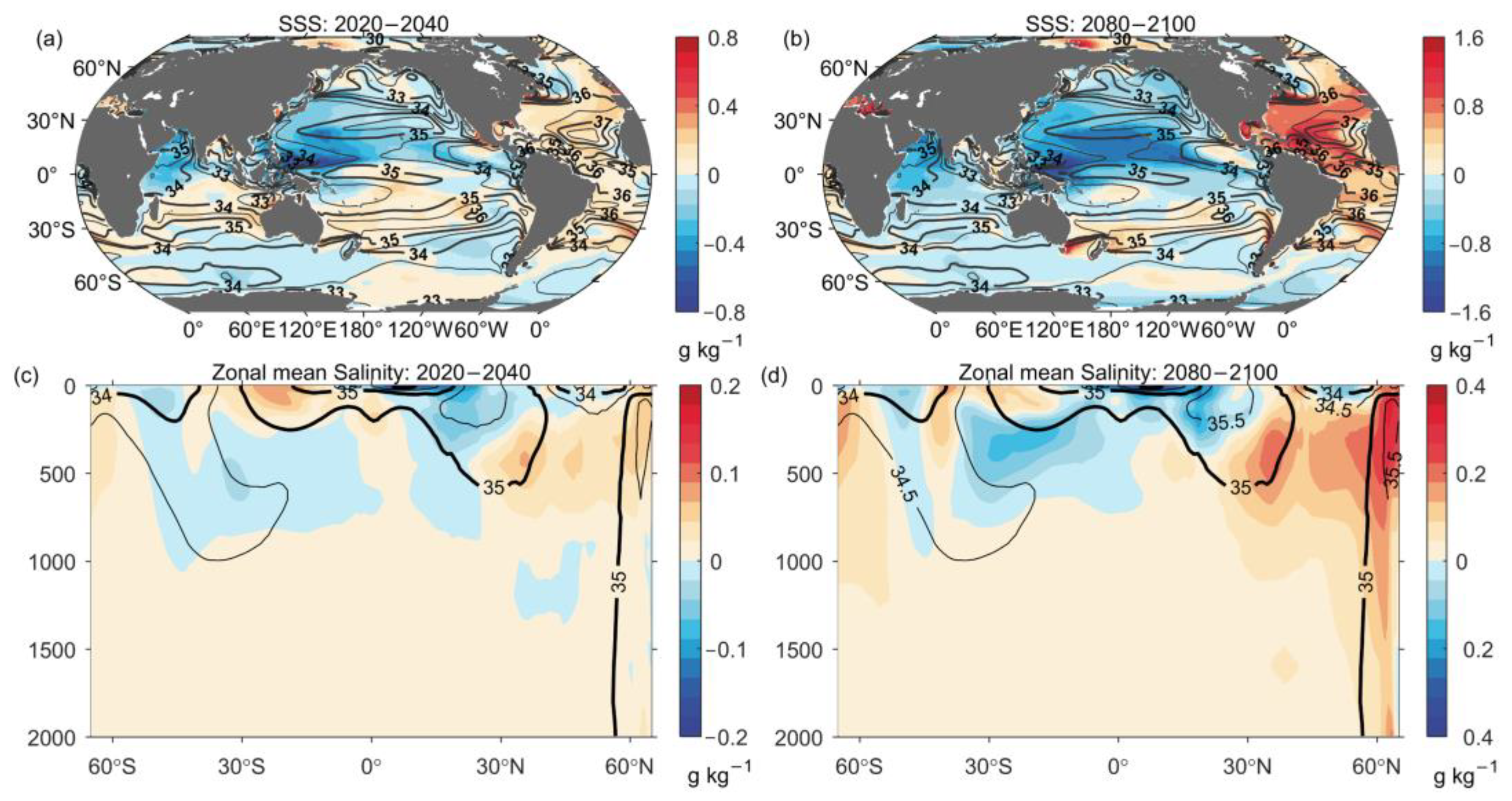
To further investigate the regional response of ocean salinity for CAS-ESM2-0 in future warming under SSP5-8.5, we assessed the spatial distribution of near-term (2020–2040) and long-term (2080–2100) salinity anomalies relative to 1990–2010 mean values (Figure 8). Both future changes in SSS indicate an overall amplified salinity pattern compared with the 1990–2010 mean state, and the magnitude of the long-term salinity anomalies is much stronger than the near-term projections. The inter-basin SSS contrast between the Atlantic and Pacific continues to increase, indicating intensified water transport under global warming (Figure 8a,b). At the end of this century, the greatest salinity increase is evident in the entire Atlantic Ocean, except south of 40° S and the Gulf Stream extension regions (~50° N). The signal of salinity increases extends to an 800 m depth within 30° N–60° N and even reaches 2000 m north of 60° N. Near-term freshening is found in the tropical western Pacific and northern Pacific Ocean (5° N–40° N) and becomes broader and stronger in the end-of-century ocean salinity pattern. This freshening extends to the upper 300 m of the low-latitude Pacific (5° S–30° N). The Pacific salinity increase in the long-term projections moves poleward in both hemispheres, and the northern signal is negligible (Figure 8b,d).
4. Conclusions and Discussion
This study evaluated the performance of salinity for the coupled CAS-ESM2-0 model at different time scales, including climatology, seasonal variation, long-term linear trends, the projection of time series, and patterns in salinity, by comparing with the ensemble mean of four observational datasets, namely, IAP, EN4, Ishii, and NCEI.
The coupled CAS-ESM2-0 model can reproduce the basin-scale ocean salinity changes, such as the mean state of the SSS and S2000 patterns, subsurface salinity pattern, and seasonal variation of SSS and S1000. The inter-basin salinity contrast between the fresher Pacific and the salty Atlantic Ocean was also demonstrated. However, fresh biases for the mean state occurred in most of the surface and subsurface layers of the global ocean, particularly in the Southern Hemisphere. The large, fresher errors (>0.5 g kg–1) in the low- and mid-latitudes in the Southern Hemisphere extended to the 500 m depth. The dipole SSS pattern of the North Indian Ocean with saltier (fresher) water in the AS (BoB) and the high salinity values for S2000 in the North Indian Ocean could not be indicated by the CAS-ESM2-0 model because of the large fresh bias in the North Indian Ocean. The CAS-ESM2-0 model displayed a stronger seasonal variation of SSS than observations, particularly in the tropics within 20° S–20° N and south of 60° S, while the variation is weaker north of 60° N. The seasonal variations of the simulated S1000 indicated a large uncertainty with the zonal band and fine structures with a similar magnitude to the observational results. The results suggest that the model still has low confidence in assessing seasonal variations of subsurface salinity, particularly at high latitudes (north of 60° N), similar to the results of other CMIP6 models [32].
In terms of the long-term linear trends, compared with the observations, the model has a similar magnitude of SSS, S2000, and global zonal mean of salinity, and it captured the increasing trends of the salinity contrast between the saltier Atlantic and fresher Pacific Ocean. However, it also revealed some regional differences in locations and strengths from the observations, such as the freshening in the North Indian Ocean, salinity increases in the Northwest Pacific and Southern Oceans, and positive trends in the upper 700 m, suggesting a negligible uncertainty in simulating and understanding regional variability.
We also investigated the performance of the CAS-ESM2-0 model in simulating and predicting the salinity change in response to global warming, including the time variation of climate metrics for salinity pattern amplification and the spatial pattern of projected salinity over the near-term (2020–2040) and long-term (2080–2100) period. The time series of the SSS-contrast and S2000-contrast indexes for the CAS-ESM2-0 model showed good consistency with the results from observations and increased substantially over the 1960–2020 period. The projected variations in SSS and S2000 indicated the persistent intensification of salinity pattern amplification until 2100. Highlighting the amplification of the global hydrological cycle in the future under the strongest forcing of the SSP5-8.5 pathway. The spatial distribution of SSS and global zonal mean of subsurface salinity over these two periods predicted an overall amplified mean salinity pattern compared to the 1990–2010 mean state and simulated the large-scale features for the inter-basin SSS contrast with broader and stronger freshening (more saline) in the Pacific (Atlantic) Ocean at the end of this century. In the Pacific, the salinity increases for long-term projections were predicted to move poleward in both hemispheres, and the salinity increase in the subtropical northern Pacific was very weak, which differs from the amplified mean salinity pattern. Our assessment provides new features of the CAS-ESM2-0 model and its errors in simulating ocean salinity and supports further studies in model development.
Some key modifications in the CAS-ESM2-0 model have been described in previous studies on ocean components, such as a new SSS boundary condition based on the physical processes of air-sea flux exchange [47], a new formulation of turbulent air-sea fluxes [48], and parameterization with a relatively more realistic sea ice salinity budget [49]. Therefore, evaluating the model performance of ocean salinity at all time scales from seasonal to multidecadal scales provides a useful reference for understanding the ability and improvement of CAS-ESM2-0 in simulating ocean salinity change and its relationship with the water cycle and the air-sea freshwater fluxes.
In general, the coupled CAS-ESM2-0 model can reasonably reproduce the general features of ocean salinity, along with common biases shared by most CMIP6 models. As a result of the substantial uncertainties in observational datasets for the seasonal variations of S1000, the regional signals of the long-term trend in surface and subsurface salinity, the CAS-ESM2-0 model cannot be fully evaluated in this study. Making a detailed diagnostic test for model biases and comparing them with other CMIP6 model results would be an intriguing follow-up study. In addition, the projected climate metrics and patterns for ocean salinity under the SSP5-8.5 pathway indicate salinity mean amplification until 2100. Therefore, further research is required to investigate future changes in ocean salinity under different pathways to understand the response of the ocean state to climate change and its impact.
Author Contributions
Conceptualization, G.L. and L.C.; methodology, G.L.; software, G.L.; validation, G.L., L.C. and X.W.; writing—original draft preparation, G.L., L.C. and X.W.; writing—review and editing, G.L., L.C. and X.W.; visualization, G.L. All authors have read and agreed to the published version of the manuscript.
Funding
This research was funded by the Natural Science Foundation of China, grant number 42206208, the National Key Scientific and Technological Infrastructure project “Earth System Science Numerical Simulator Facility” (EarthLab), the Young Talent Support Project of Guangzhou Association for Science and Technology, and the Strategic Priority Research Program of the Chinese Academy of Sciences, grant number XDB42040402.
Institutional Review Board Statement
Not applicable.
Informed Consent Statement
Not applicable.
Data Availability Statement
The output of the CAS-ESM2-0 model are downloaded from https://esgf-node.llnl.gov/search/cmip6 (accessed on 1 September 2022). The collected salinity gridded datasets are as follows: IAP (http://www.ocean.iap.ac.cn/, accessed on 1 September 2022), NCEI (https://www.ncei.noaa.gov/access/global-ocean-heat-content/anomaly_data_s.html, accessed on 1 September 2022), EN4 (https://www.metoffice.gov.uk/hadobs/en4/download-en4-2-1.html, accessed on 1 September 2022), and Ishii (https://climate.mri-jma.go.jp/pub/ocean/ts/v7.2/, accessed on 1 September 2022). Further inquiries are available upon request.
Acknowledgments
We would like to thank WCRP (World Climate Research Program) and ESFG (Earth System Grid Federation) for making the data available for this research. We also thank the editors, reviewers, and colleagues for their constructive comments when developing this manuscript.
Conflicts of Interest
The authors declare no conflict of interest.
References
- IPCC. Climate Change 2021: The Physical Science Basis; Masson-Delmotte, V., Zhai, P., Pirani, A., Connors, S.L., Péan, C., Berger, S., Caud, N., Chen, Y., Goldfarb, L., Gomis, M.I., et al., Eds.; Cambridge University Press: Cambridge, UK; New York, NY, USA, 2021. [Google Scholar]
- Ross, E.; Behringer, D. Changes in temperature, pH, and salinity affect the sheltering responses of Caribbean spiny lobsters to chemosensory cues. Sci. Rep. 2019, 9, 4375. [Google Scholar] [CrossRef] [PubMed] [Green Version]
- Yu, L. A global relationship between the ocean water cycle and near-surface salinity. J. Geophys. Res. 2011, 116, C10025. [Google Scholar] [CrossRef]
- Eyring, V.; Bony, S.; Meehl, G.; Senior, C.; Stevens, B.; Ronald, S.; Taylor, K. Overview of the Coupled Model Intercomparison Project Phase 6 (CMIP6) experimental design and organization. Geosci. Model Dev. 2016, 9, 1937–1958. [Google Scholar] [CrossRef] [Green Version]
- Zhang, H.; Zhang, M.; Jin, J.; Fei, K.; Ji, D.; Wu, C.; Zhu, J.; He, J.; Chai, Z.; Xie, J.; et al. Description and Climate Simulation Performance of CAS-ESM Version 2. J. Adv. Model. Earth Syst. 2020, 12, e2020MS002210. [Google Scholar] [CrossRef]
- Gao, X.; Fan, P.; Jin, J.; He, J.; Song, M.; Zhang, H.; Fei, K.; Zhang, M.; Zeng, Q. Evaluation of Sea Ice Simulation of CAS-ESM 2.0 in Historical Experiment. Atmosphere 2022, 13, 1056. [Google Scholar] [CrossRef]
- Jin, J.; Zhang, H.; Dong, X.; Liu, H.; Zhang, M.; Gao, X.; He, J.; Chai, Z.; Zeng, Q.; Zhou, G.; et al. CAS-ESM2.0 Model Datasets for the CMIP6 Flux-Anomaly-Forced Model Intercomparison Project (FAFMIP). Adv. Atmos. Sci. 2021, 38, 296–306. [Google Scholar] [CrossRef]
- Zhang, W.; Xue, F.; Jin, J.; Dong, X.; Zhang, H.; Lin, R. Comparison of East Asian Summer Monsoon Simulation between an Atmospheric Model and a Coupled Model: An Example from CAS-ESM. Atmosphere 2022, 13, 998. [Google Scholar] [CrossRef]
- Li, J.; Su, J. Comparison of Indian Ocean warming simulated by CMIP5 and CMIP6 models. Atmos. Ocean. Sci. Lett. 2020, 13, 604–611. [Google Scholar] [CrossRef]
- Tian, B.; Dong, X. The Double-ITCZ Bias in CMIP3, CMIP5, and CMIP6 Models Based on Annual Mean Precipitation. Geophys. Res. Lett. 2020, 47, e2020GL087232. [Google Scholar] [CrossRef] [Green Version]
- Tsujino, H.; Urakawa, L.S.; Griffies, S.M.; Danabasoglu, G.; Adcroft, A.J.; Amaral, A.E.; Arsouze, T.; Bentsen, M.; Bernardello, R.; Böning, C.W.; et al. Evaluation of global ocean-sea-ice model simulations based on the experimental protocols of the Ocean Model Intercomparison Project phase 2 (OMIP-2). Geosci. Model Dev. 2020, 13, 3643–3708. [Google Scholar] [CrossRef]
- Chassignet, E.P.; Yeager, S.G.; Fox-Kemper, B.; Bozec, A.; Castruccio, F.; Danabasoglu, G.; Horvat, C.; Kim, W.M.; Koldunov, N.; Li, Y.; et al. Impact of horizontal resolution on global ocean–sea ice model simulations based on the experimental protocols of the Ocean Model Intercomparison Project phase 2 (OMIP-2). Geosci. Model Dev. 2020, 13, 4595–4637. [Google Scholar] [CrossRef]
- Trenberth, K.E.; Stepaniak, D.P. Indices of El Niño Evolution. J. Clim. 2001, 14, 1697–1701. [Google Scholar] [CrossRef]
- Chen, H.-C.; Jin, F.-F. Simulations of ENSO Phase-Locking in CMIP5 and CMIP6. J. Clim. 2021, 34, 5135–5149. [Google Scholar] [CrossRef]
- Sharma, R.; Agarwal, N.; Momin, I.M.; Basu, S.; Agarwal, V.K. Simulated Sea Surface Salinity Variability in the Tropical Indian Ocean. J. Clim. 2010, 23, 6542–6554. [Google Scholar] [CrossRef]
- Kido, S.; Tozuka, T.; Han, W. Experimental Assessments on Impacts of Salinity Anomalies on the Positive Indian Ocean Dipole. J. Geophys. Res. Ocean. 2019, 124, 9462–9486. [Google Scholar] [CrossRef]
- Zhu, J.; Huang, B.; Zhang, R.; Hu, Z.; Kumar, A.; Balmaseda, M.A.; Marx, L.; Kinter, J.L. Salinity anomaly as a trigger for ENSO events. Sci. Rep. 2014, 4, 6821. [Google Scholar] [CrossRef] [Green Version]
- Ke-xin, L.; Fei, Z. Effects of a freshening trend on upper-ocean stratification over the central tropical Pacific and their representation by CMIP6 models. Deep Sea Res. Part II Top. Stud. Oceanogr. 2022, 195, 104999. [Google Scholar] [CrossRef]
- Zheng, F.; Zhang, R. Interannually varying salinity effects on ENSO in the tropical pacific: A diagnostic analysis from Argo. Ocean Dyn. 2015, 65, 691–705. [Google Scholar] [CrossRef]
- Zhi, H.; Zhang, R.-H.; Lin, P.; Yu, P. Interannual Salinity Variability in the Tropical Pacific in CMIP5 Simulations. Adv. Atmos. Sci. 2019, 36, 378–396. [Google Scholar] [CrossRef]
- Liu, H.; Lin, P.; Yu, Y.; Zhang, X.J.A.M.S. The baseline evaluation of LASG/IAP climate system ocean model (LICOM) version 2. Acta Meteorol. Sin. 2012, 26, 318–329. [Google Scholar] [CrossRef]
- Hunke, E.C.; Lipscomb, W.H. CICE: The Los Alamos Sea Ice Model User’s Manual, Version 4; LA-CC-06-012; Los Alamos National Laboratory Tech. Rep.: Los Alamos, NM, USA, 2008.
- Dai, Y.; Zeng, X.; Dickinson, R.E.; Baker, I.; Bonan, G.B.; Bosilovich, M.G.; Denning, A.S.; Dirmeyer, P.A.; Houser, P.R.; Niu, G.; et al. The Common Land Model. Bull. Am. Meteorol. Soc. 2003, 84, 1013–1024. [Google Scholar] [CrossRef] [Green Version]
- He, J.; Zhang, M.; Lin, W.; Colle, B.; Liu, P.; Vogelmann, A.M. The WRF nested within the CESM: Simulations of a midlatitude cyclone over the Southern Great Plains. J. Adv. Model. Earth Syst. 2013, 5, 611–622. [Google Scholar] [CrossRef]
- O’Neill, B.C.; Tebaldi, C.; van Vuuren, D.P.; Eyring, V.; Friedlingstein, P.; Hurtt, G.; Knutti, R.; Kriegler, E.; Lamarque, J.F.; Lowe, J.; et al. The Scenario Model Intercomparison Project (ScenarioMIP) for CMIP6. Geosci. Model Dev. 2016, 9, 3461–3482. [Google Scholar] [CrossRef] [Green Version]
- Cheng, L.; Trenberth, K.E.; Gruber, N.; Abraham, J.P.; Fasullo, J.T.; Li, G.; Mann, M.E.; Zhao, X.; Zhu, J. Improved Estimates of Changes in Upper Ocean Salinity and the Hydrological Cycle. J. Clim. 2020, 33, 10357–10381. [Google Scholar] [CrossRef]
- Good, S.A.; Martin, M.; Rayner, N.A. EN4: Quality controlled ocean temperature and salinity profiles and monthly objective analyses with uncertainty estimates. J. Geophys. Res. 2013, 118, 6704–6716. [Google Scholar] [CrossRef]
- Levitus, S.; Antonov, J.I.; Boyer, T.P.; Baranova, O.K.; Garcia, H.E.; Locarnini, R.A.; Mishonov, A.V.; Reagan, J.R.; Seidov, D.; Yarosh, E.S.; et al. World ocean heat content and thermosteric sea level change (0–2000 m), 1955–2010. Geophys. Res. Lett. 2012, 39, L10603. [Google Scholar] [CrossRef] [Green Version]
- Boyer, T.P.; Levitus, S.; Antonov, J.I.; Locarnini, R.A.; Garcia, H.E. Linear trends in salinity for the World Ocean, 1955–1998. Geophys. Res. Lett. 2005, 32, 67–106. [Google Scholar] [CrossRef] [Green Version]
- Ishii, M.; Kimoto, M. Reevaluation of historical ocean heat content variations with time-varying XBT and MBT depth bias corrections. J. Oceanogr. 2009, 65, 287–299. [Google Scholar] [CrossRef]
- Foster, G.; Rahmstorf, S. Global temperature evolution 1979–2010. Environ. Res. Lett. 2011, 6, 044022. [Google Scholar] [CrossRef]
- Liu, Y.; Cheng, L.; Pan, Y.; Tan, Z.; Abraham, J.; Zhang, B.; Zhu, J.; Song, J. How Well Do CMIP6 and CMIP5 Models Simulate the Climatological Seasonal Variations in Ocean Salinity? Adv. Atmos. Sci. 2022, 39, 1650–1672. [Google Scholar] [CrossRef]
- Durack, P.J.; Wijffels, S.E.; Matear, R.J. Ocean salinities reveal strong global water cycle intensification during 1950 to 2000. Science 2012, 336, 455. [Google Scholar] [CrossRef] [PubMed] [Green Version]
- Zhou, G.; Zhang, Y.; Jiang, J.; Zhang, H.; Wu, B.; Cao, H.; Wang, T.; Hao, H.; Zhu, J.; Yuan, L.; et al. Earth System Model: CAS-ESM. Front. Data Comput. 2020, 2, 38–54. [Google Scholar] [CrossRef]
- Durack, P.J.; Wijffels, S.E. Fifty-year trends in global ocean salinities and their relationship to broad-scale warming. J. Clim. 2010, 23, 4342–4362. [Google Scholar] [CrossRef]
- Rahaman, H.; Srinivasu, U.; Panickal, S.; Durgadoo, J.V.; Griffies, S.M.; Ravichandran, M.; Bozec, A.; Cherchi, A.; Voldoire, A.; Sidorenko, D.; et al. An assessment of the Indian Ocean mean state and seasonal cycle in a suite of interannual CORE-II simulations. Ocean Model. 2020, 145, 101503. [Google Scholar] [CrossRef]
- Dwivedi, S.; Mishra, A.K.; Srivastava, A. Upper ocean high resolution regional modeling of the Arabian Sea and Bay of Bengal. Acta Oceanol. Sin. 2019, 38, 32. [Google Scholar] [CrossRef]
- Srivastava, A.; Dwivedi, S.; Mishra, A.K. Investigating the role of air-sea forcing on the variability of hydrography, circulation, and mixed layer depth in the Arabian Sea and Bay of Bengal. Oceanologia 2018, 60, 169–186. [Google Scholar] [CrossRef]
- Curry, R.; Dickson, B.; Yashayaev, I. A change in the freshwater balance of the Atlantic Ocean over the past four decades. Nature 2003, 426, 826. [Google Scholar] [CrossRef] [PubMed]
- Liu, Y.; Cheng, L.; Pan, Y.; Abraham, J.; Zhang, B.; Zhu, J.; Song, J. Climatological seasonal variation of the upper ocean salinity. Int. J. Climatol. 2021, 42, 3477–3498. [Google Scholar] [CrossRef]
- Dong, X.; Jin, J.; Liu, H.; Zhang, H.; Zhang, M.; Lin, P.; Zeng, Q.; Zhou, G.; Yu, Y.; Song, M.; et al. CAS-ESM2.0 Model Datasets for the CMIP6 Ocean Model Intercomparison Project Phase 1 (OMIP1). Adv. Atmos. Sci. 2021, 38, 307–316. [Google Scholar] [CrossRef]
- Eyring, V.; Gillett, N.; Achuta Rao, K.; Barimalala, R.; Barreiro Parrillo, M.; Bellouin, N.; Cassou, C.; Durack, P.; Kosaka, Y.; McGregor; et al. Human Influence on the Climate System: Contribution of Working Group I to the Sixth Assessment Report of the Intergovernmental Panel on Climate Change. 2021. Available online: https://www.ipcc.ch/report/ar6/wg1/ (accessed on 1 September 2022).
- Reagan, J.; Seidov, D.; Boyer, T. Water Vapor Transfer and Near-Surface Salinity Contrasts in the North Atlantic Ocean. Sci. Rep. 2018, 8, 8830. [Google Scholar] [CrossRef]
- Sprintall, J.; Siedler, G.; Mercier, H. Chapter 19–Interocean and Interbasin Exchanges. Int. Geophys. 2013, 103, 493–518. [Google Scholar]
- Lovato, T.; Peano, D.; Butenschön, M.; Materia, S.; Iovino, D.; Scoccimarro, E.; Fogli, P.G.; Cherchi, A.; Bellucci, A.; Gualdi, S.; et al. CMIP6 simulations with the CMCC Earth System Model (CMCC-ESM2). J. Adv. Model. Earth Syst. 2022, 14, e2021MS002814. [Google Scholar] [CrossRef]
- Jan, D.Z.; Nikolaos, S.; Adam, T.B.; Robert, M.; Nurser, A.J.G.; Josey, S.A. Improved estimates of water cycle change from ocean salinity: The key role of ocean warming. Environ. Res. Lett. 2018, 13, 074036. [Google Scholar] [CrossRef] [Green Version]
- Jin, J.; Zeng, Q.; Wu, L.; Liu, H.; Zhang, M. Formulation of a new ocean salinity boundary condition and impact on the simulated climate of an oceanic general circulation model. Sci. China Earth Sci. 2017, 60, 491–500. [Google Scholar] [CrossRef]
- Fairall, C.W.; Bradley, E.F.; Hare, J.E.; Grachev, A.A.; Edson, J.B. Bulk Parameterization of Air–Sea Fluxes: Updates and Verification for the COARE Algorithm. J. Clim. 2003, 16, 571–591. [Google Scholar] [CrossRef]
- Liu, J. Sensitivity of sea ice and ocean simulations to sea ice salinity in a coupled global climate model. Sci. China Earth Sci. 2010, 53, 911–918. [Google Scholar] [CrossRef]
Figure 1.
Global climatology of (a) the sea surface salinity (SSS) and (b) 0–2000 m averaged salinity (S2000) for the ensemble means of the four observational products, (c,d) for the CAS-ESM2-0 model. The difference between the model and observational mean is shown in (e,f), respectively.
Figure 1.
Global climatology of (a) the sea surface salinity (SSS) and (b) 0–2000 m averaged salinity (S2000) for the ensemble means of the four observational products, (c,d) for the CAS-ESM2-0 model. The difference between the model and observational mean is shown in (e,f), respectively.

Figure 2.
Global climatology of the global zonal mean salinity from the surface to 2000 m: (a) for the ensemble means of the four observational products and (b) the CAS-ESM2-0 model. (c) The difference between the model and observational mean.
Figure 2.
Global climatology of the global zonal mean salinity from the surface to 2000 m: (a) for the ensemble means of the four observational products and (b) the CAS-ESM2-0 model. (c) The difference between the model and observational mean.

Figure 3.
Global zonal mean of the seasonal variation of the (a) sea surface salinity (SSS) and (b) 0–1000 m averaged salinity (S1000) for the observational mean, (c,d) for CAS-ESM2-0 model. The differences between the model and observational mean are shown in (e,f), respectively. The monthly anomalies are obtained from the 12-month climatological means, which has removed the annual mean during 1990–2010.

Figure 4.
Seasonal variation magnitudes of the (a) sea surface salinity (SSS) and (b) 0–1000 m averaged salinity (S1000) for the observational mean, (c,d) for the CAS-ESM2-0 model. Mean differences between the model and observational mean in summer and winter for the (e,g) SSS and (f,h) S1000. The monthly anomalies are obtained from the 12-month climatological means, which has removed the annual mean during 1990–2010. The magnitude of seasonal variation is defined by the standard deviation of time variation. The averages of summer and winter are obtained for June-July-August and December-January-February, respectively.

Figure 5.
Linear trends of the (a) sea surface salinity (SSS) and (b) 0–2000 m averaged salinity (S2000) anomalies during 1960–2020 for the observational mean, (c,d) for the CAS-ESM2-0 model. The anomalies are relative to the 1990–2010 baseline. The stippling indicates the regions with statically significant signals (95% confidence level). Mean differences between the model and observational mean for the (e) SSS and (f) S2000.

Figure 6.
Linear trends of the globally zonal-mean salinity anomalies during 1960-2020: (a) for the ensemble means of the four observational products, (b) for CAS-ESM2-0 model. The unit of salinity is g kg−1 per year. The anomalies are relative to the 1990–2010 baseline. The stippling indicates the regions with statically significant signals (95% confidence level).

Figure 7.
Time series of the global annual mean for (a) sea surface salinity (SSS) contrast and (b) 0-2000 m averaged salinity (S2000) contrast metrics as monitored from the IAP observation (solid black line) and as simulated by CAS-ESM2-0 in historical and SSP5-8.5 projections during 1960–2100 (solid red line). The gray shadings denote 2 times standard deviation of error range in IAP mapping framework. The color lines are the time series after applying the LOWESS (locally weighted scatterplot smoothing) smoother with a span width of 3 years.

Figure 8.
Projection of spatial patterns of period differences of sea surface salinity (SSS) anomaly (left panels) and global zonal mean of subsurface salinity anomaly from the surface to 2000 m (right panels) for CAS-ESM2-0 model under SSP5-8.5 between the period of 2020–2040 (a,c), 2080–2100 (b,d), and 1960–1980. The black contours denote CAS-ESM2-0 historical climatology averaged between 1990–2010. Anomalies are the period’s mean values relative to the 1990–2010 baseline period.

Disclaimer/Publisher’s Note: The statements, opinions and data contained in all publications are solely those of the individual author(s) and contributor(s) and not of MDPI and/or the editor(s). MDPI and/or the editor(s) disclaim responsibility for any injury to people or property resulting from any ideas, methods, instructions or products referred to in the content. |
© 2023 by the authors. Licensee MDPI, Basel, Switzerland. This article is an open access article distributed under the terms and conditions of the Creative Commons Attribution (CC BY) license (https://creativecommons.org/licenses/by/4.0/).
Share and Cite
MDPI and ACS Style
Li, G.; Cheng, L.; Wang, X. Evaluation of the CAS-ESM2-0 Performance in Simulating the Global Ocean Salinity Change. Atmosphere 2023, 14, 107. https://doi.org/10.3390/atmos14010107
AMA Style
Li G, Cheng L, Wang X. Evaluation of the CAS-ESM2-0 Performance in Simulating the Global Ocean Salinity Change. Atmosphere. 2023; 14(1):107. https://doi.org/10.3390/atmos14010107
Chicago/Turabian StyleLi, Guancheng, Lijing Cheng, and Xutao Wang. 2023. "Evaluation of the CAS-ESM2-0 Performance in Simulating the Global Ocean Salinity Change" Atmosphere 14, no. 1: 107. https://doi.org/10.3390/atmos14010107
Note that from the first issue of 2016, this journal uses article numbers instead of page numbers. See further details here.