
Estimation of the Number of Sprites Observed over Japan in 5.5 Years Using Lightning Data

Department of Physical Science, Aoyama Gakuin University, Sagamihara 252-5258, Kanagawa, Japan
*
Author to whom correspondence should be addressed.
Atmosphere 2023, 14(1), 105; https://doi.org/10.3390/atmos14010105
Submission received: 29 November 2022
/
Revised: 23 December 2022
/
Accepted: 28 December 2022
/
Published: 3 January 2023
(This article belongs to the Section Upper Atmosphere)
Abstract
:This study is based on 5.5 years of continuous observation of sprites from Sagamihara, Japan. Up to February 2022, we detected 537 sprites and found that the most significant number of sprites were observed during the winter (303 sprites); on the other hand, there were only 46 sprites in summer. The hourly distribution of the number of observed sprites peaked at midnight JST (15:00 and 16:00 UTC). To understand the seasonal and the hourly distribution of sprites, we estimate the number of sprites considering the energy and the polarity of lightning, the temporal changes of surrounding environments of sprites, and the conditions for generating sprites. We found that the energy of lightning, the monthly ratio of a positive cloud-to-ground discharge, and the hourly change in the electron number density are essential factors to match the observed sprite distributions.
1. Introduction
Sprites are luminous phenomena caused by lightning strokes, which occur at an altitude of 50–90 km [1,2,3]. They are also called red sprites, as they have a short emission time, disappear instantly, and are red in color. As a primary generation mechanism, a positive cloud-to-ground discharge (+CG) applies a quasi-electrostatic field above the thundercloud, accelerates electrons, and emits light when they collide with the neutral air [4,5]. Pasko et al. [5] have pointed out that a charge moment change (CMC) is the most critical factor for generating sprites. The minimum reliably recorded CMC is 120 C·km [6]. According to the observations of Hobara et al. [7] and Hayakawa et al. [8], the minimum CMC of winter sprites in Japan is 200–300 C·km. Additionally, according to the statistical results of Hu et al. [6], if a CMC of +CGs exceeds 1000 C·km within 6 ms after discharge, the probability of a sprite occurring reaches 90%. On the other hand, if a CMC does not exceed 600 C·km, the probability of a sprite occurring is as low as 10%. In addition, Cummer and Lyons [9] have pointed out that, if a CMC exceeds 600 C·km, the probability of sprite occurrence will increase sharply.
The number of sprites varies by region and season [10]; for example, many winter sprites are observed over the Sea of Japan and the Hokuriku of Japan, but there are very few summer sprites [8,11]. This is due to the fraction of +CGs during summer being only about 10%, but this number reaches about 50% in winter [12,13]. Furthermore, +CGs during the winter in Japan can transfer massive charges to the ground [12,13,14]. Therefore, winter sprites are abundant over the Sea of Japan and the Hokuriku of Japan. On the other hand, summer sprites over Japan are very scarce [8].
Sprites are typically observed at night. However, on 14 August 1998, Stanley et al. [15] reported the detection of three sprites during the daytime at low frequency. The +CGs generating the three sprites were CMCs greater than 2800, 1200, and 910 C·km. These CMCs were abnormally more significant than those associated with sprites observed at night. According to Stanley et al. [15], the electron number density in the ionospheric D layer during the daytime was two orders of magnitude higher than that at night-time and, so, the electrical conductivity of air was also enormous. As a necessary condition for sprites, the relaxation time must be maintained at a constant time. However, is shortened with increasing [4,5]. When is relatively small, a large CMC is needed to maintain constantly. Therefore, the requirement of a CMC for daytime sprites is larger, and sprites are less likely to occur during the daytime.
Evtushenko et al. [16] have calculated the probability that each lightning strike could trigger a sprite at night, using the World Wide Lightning Location Network (WWLLN; [17,18,19]) data to estimate the number and the global distribution of sprites. According to Evtushenko et al. [16], 870 night-time sprites occur worldwide every 24 h. Of these, 41.4% occurred on land and 58.6% at sea. The number of estimated sprites worldwide is the largest in August and the smallest in January and February.
In this paper, we present the monthly and hourly distribution of sprites around Japan through 5.5 years of observations. We also present an estimate of the number of sprites using the WWLLN data. In Section 2, we present the results of 5.5 years of sprite observations in Japan. In Section 3, we detail our first attempt to estimate the number of sprites from the WWLLN data. In Section 4, based on the study of Section 3, we update the model to estimate the number of sprites by considering the temporal variation of several key parameters. Finally, we discuss and conclude our study in Section 5.
2. Sprite Observations in Japan over 5.5 Years
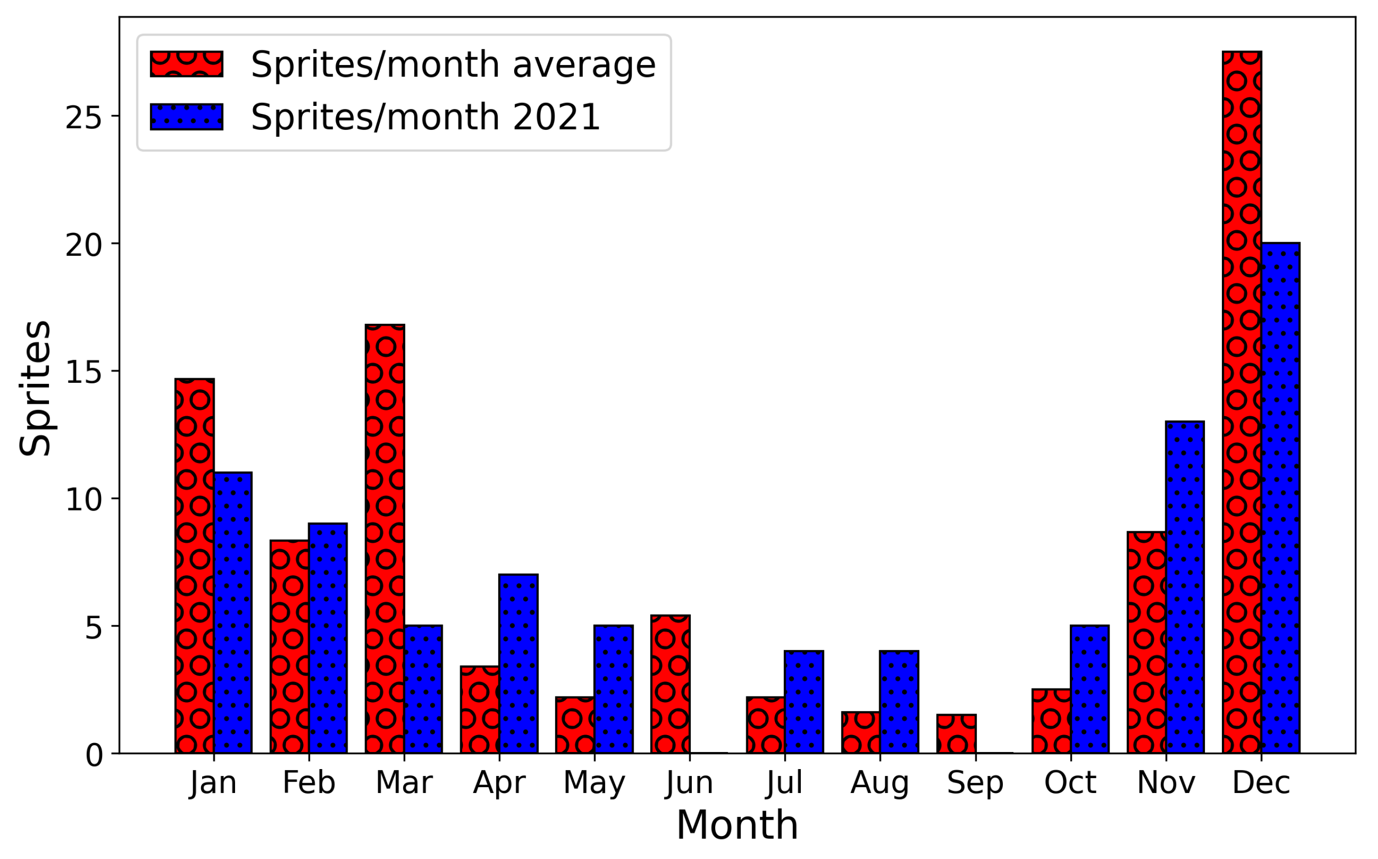
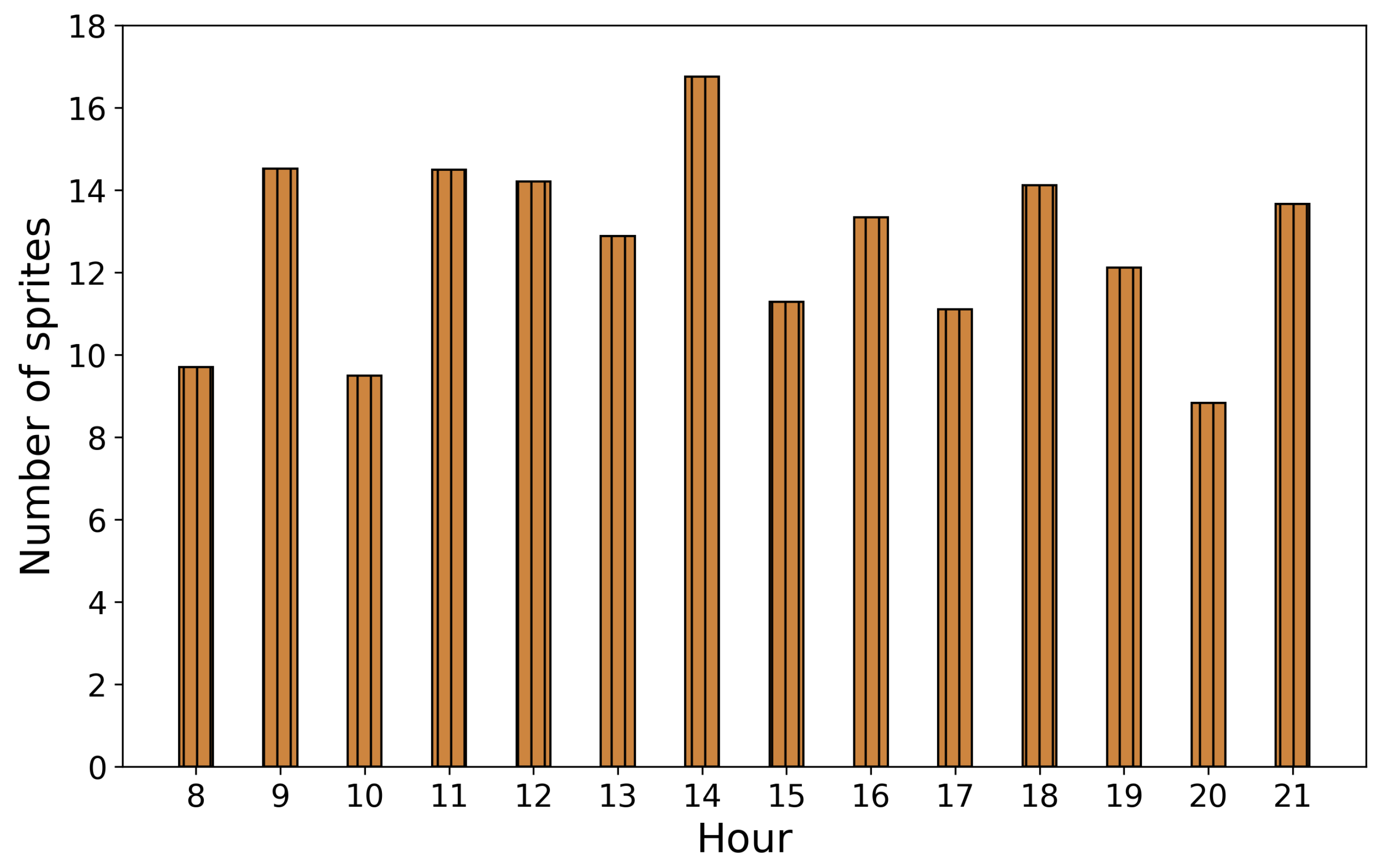
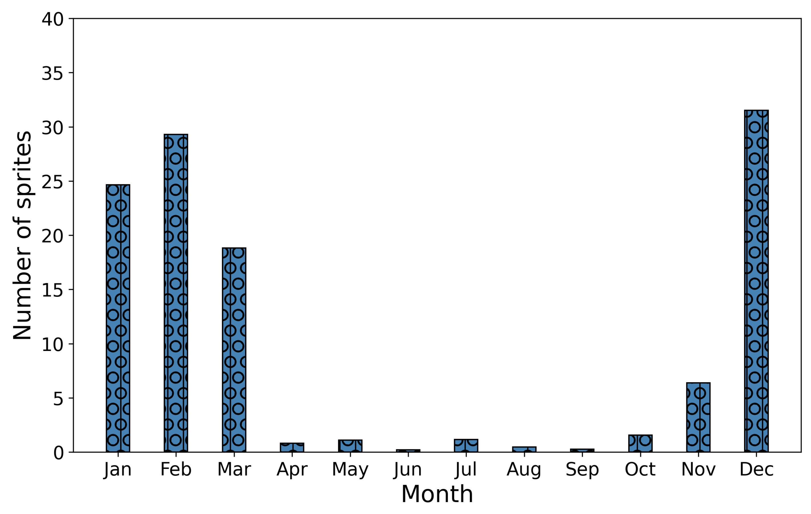
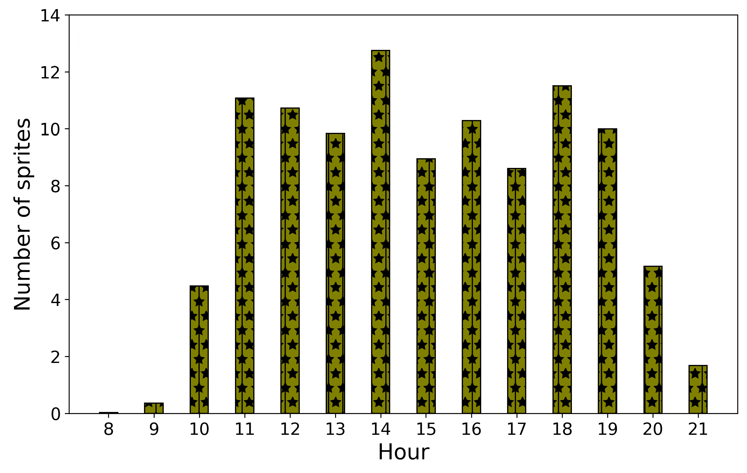
Starting from September 2016, we installed three wide-field optical cameras, which we named Aoyama Gakuin University Sprite Camera (ASCA), at Sagamihara, Japan (35.57 N, 139.40 E), which observed from sunset to sunrise in JST (8:00–21:00 UTC). Up to February 2022, ASCA detected 537 sprites in total. Figure 1 shows the monthly distribution of the observed sprites. The distribution is the largest in winter, with 303 sprites, accounting for 56% of the total. On the other hand, there are only 46 sprites in summer (9% of the total). December has the most significant number, with 165 sprites, exceeding 30% of the whole. January and March follow, with 88 and 84 sprites, respectively, accounting for 16% each of the total. August and September are the lowest, with 8 and 9 sprites, respectively. Figure 2 shows the hourly distribution of the observed sprites. The distribution peaks at midnight JST (15:00 and 16:00 UTC). The number of observed sprites at 15:00 and 16:00 UTC is 74 and 75 sprites, respectively, accounting for 28% of the total. The complete catalog of 537 sprites will be presented elsewhere.
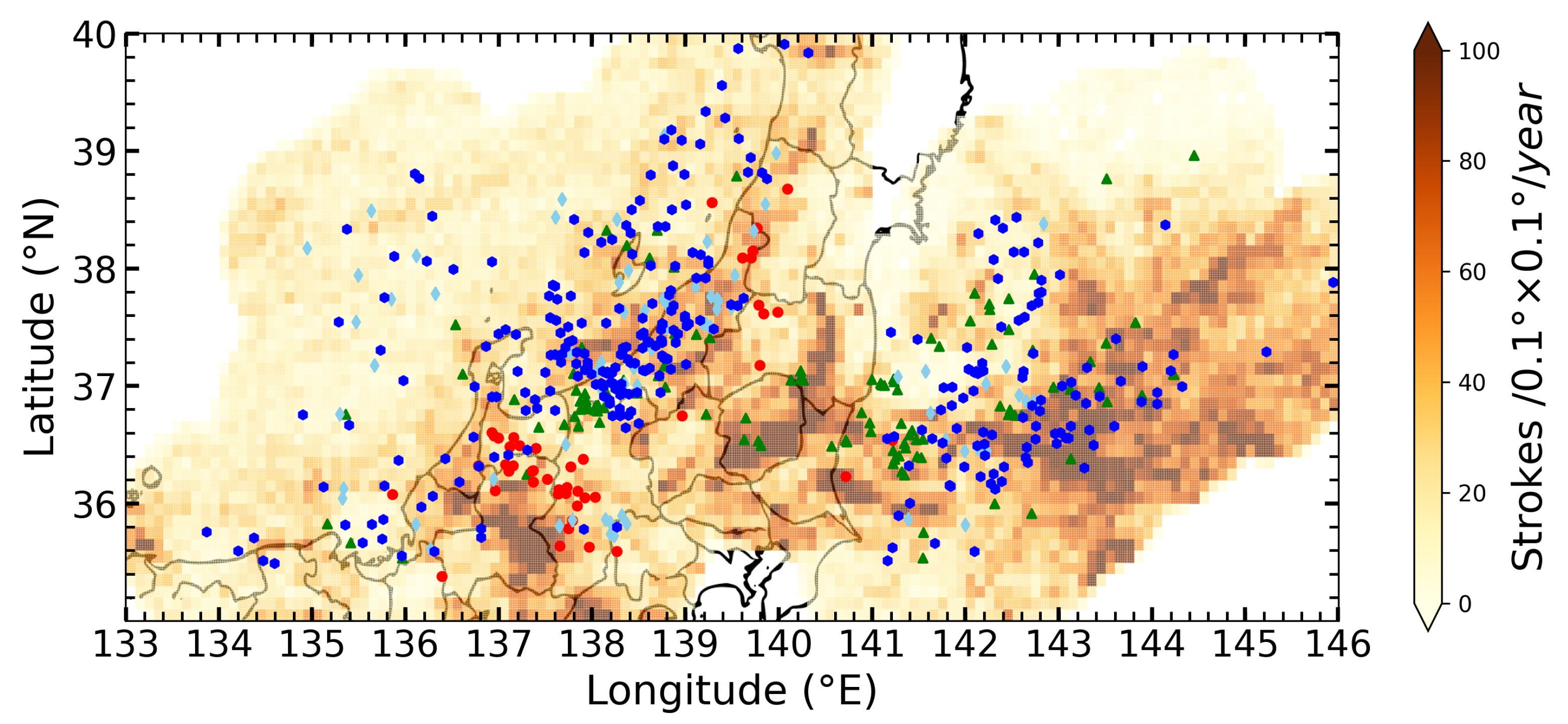
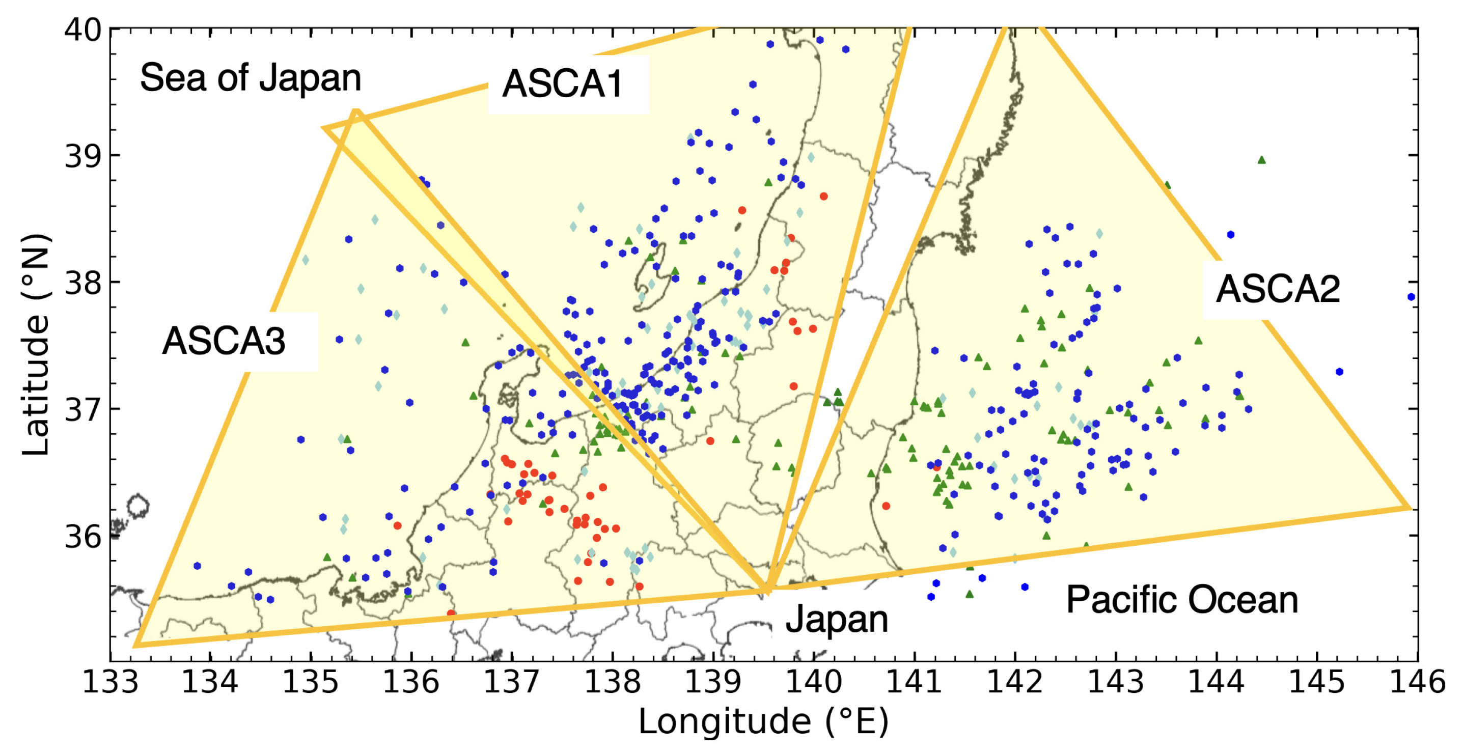
Figure 3 summarizes the locations of the 537 sprites observed from September 2016 to February 2022. Figure 4 overlays the fields of view for each ASCA camera. As shown in Figure 4, there is an uncovered area at the northeast coast and the entire west of Japan from Sagamihara, due to the limited view from the site. Overall, sprites are concentrated along the coast of the Sea of Japan and distributed in large numbers on the Pacific Ocean side. There are 181 sprites detected on the Pacific side, accounting for 34% of the total. Unlike other seasons, the 46 summer sprites (red dots) are concentrated in the mainland of Japan, and only four of them are detected in the sea near the coastline. Figure 3 also overlays the lightning strikes per unit area (0.1× 0.1) over Japan in 2021, as observed by the WWLLN, within 100 km from the locations of the sprites. The lightning data we used are limited to the time range of 8:00–21:00 UTC, consistent with the time window of the observed sprites. The sprite locations generally present good agreement with the high-density lightning area.
3. Estimation of the Number of Sprites
Evtushenko et al. [16] have used WWLLN data from 2016 to estimate the number of sprites occurring worldwide during the night. We use the model of Evtushenko et al. [16] to calculate the number of sprites in Japan, and compare the result with the actual observed data. The WWLLN data for 2021 are used in our analysis. Solar radiation increases the ionosphere electron density during the day, and electron density affects the production of sprites [15]. In addition, due to the strong sunlight, even if sprites are generated, it would be difficult to capture them with our cameras. Therefore, our observed time frame in the analysis is during the night in Japan (8:00–21:00 UTC). Considering the limited range of ASCA observations, we use the WWLLN data within 100 km from the sprites detected by ASCA, as shown in Figure 3.
3.1. Sprite Number Estimation Model
First, we estimate the peak current from the WWLLN energy data. Second, we calculate the impulse charge moment change (iCMC) from a peak current, where an iCMC is a CMC within 2 ms after a discharge. As many simulations assume a discharge time of 2 ms, the iCMC is the same as the CMC in our calculations. Third, we set the +CG and a negative cloud-to-ground discharge (−CG) ratio. Fourth, we estimate the sprite generation probability for a single strike by substituting the iCMC into a sprite generation probability equation. Finally, the number of positive and negative sprites is estimated by multiplying a polarity ratio.
The WWLLN provides an empirical equation that estimates a peak current I from RMS energy [20]. We calculate the root-mean-square (RMS) energy from the energy of the lightning strike. The equation used to calculate I is as follows:
where the unit of I is kA. When the iCMC or CMC is small, sprites do not occur. Therefore, we exclude the situation where the energy and peak current of lightning are negligible. Considering the results of Lu et al. [21], Cummer et al. [22], and Lu et al. [23], Evtushenko et al. [16] estimated the following expressions between peak current and iCMC:
where positive denotes calculating the iCMC of a positive peak current, while negative denotes calculating the iCMC of a negative peak current.
The threshold of positive sprites generated by +CGs is low, as +CGs and −CGs have different sprite production mechanisms; that is, positive sprites are more likely to occur than negative sprites. Therefore, the polarity of the CG is essential for estimating the number of sprites. The ratio of +CGs, R, can be obtained from long-running regional lightning observation systems such as the National Lightning Detection Network (NLDN) or the European Cooperation for Lightning Detection (EUCLID). For example, the NLDN data for 1995–1999 showed that, on average, R was 0.1 over most of the United States, rising to 0.2 in some regions [24]. Evtushenko et al. [16] assumed R = 0.1, but the R-value varies greatly between different regions and seasons. Sugita and Matsui [25] have investigated the lightning distribution, frequency, and polarity using the Japanese Lightning Detection Network (JLDN). The location range of this study was 26.5–48.5 N and 126–148 E from 2001 to 2010. As we aim to understand the number of sprites observed by ASCA, we assume the monthly R in Japan based on Sugita and Matsui [25].
For the CMC of sprites, the minimum reliably recorded value is 120 C·km, the average is 400–600 C·km, and the maximum is around 1000 C·km [6]. The numerical calculations of Qin et al. [26] showed that the minimum iCMC are 200 and 320 C·km for positive and negative sprites, respectively. Based on electric field measurements, the probability of sprite generation depends on the iCMC [27]. Cummer et al. [22] have taken into account the number of lightning flashes and the number of sprites, and argued that the thresholds were 300 and 500 C·km for positive and negative sprites, respectively. Evtushenko et al. [16] considered the above studies and simulation results, and came up with the following equation:
where a = 400 C·km for +CGs and a = 600 C·km for −CGs, both with b of 40 C·km. Evtushenko et al. [16] assumed 100 and 300 C·km as the thresholds for positive and negative sprites. Previous studies have shown that the proportion of negative sprites is less than 0.1%, and it is generally believed that +CGs cause sprites [28]. Therefore, we only estimate the number of positive sprites.
3.2. Result for the Number of Estimated Sprites
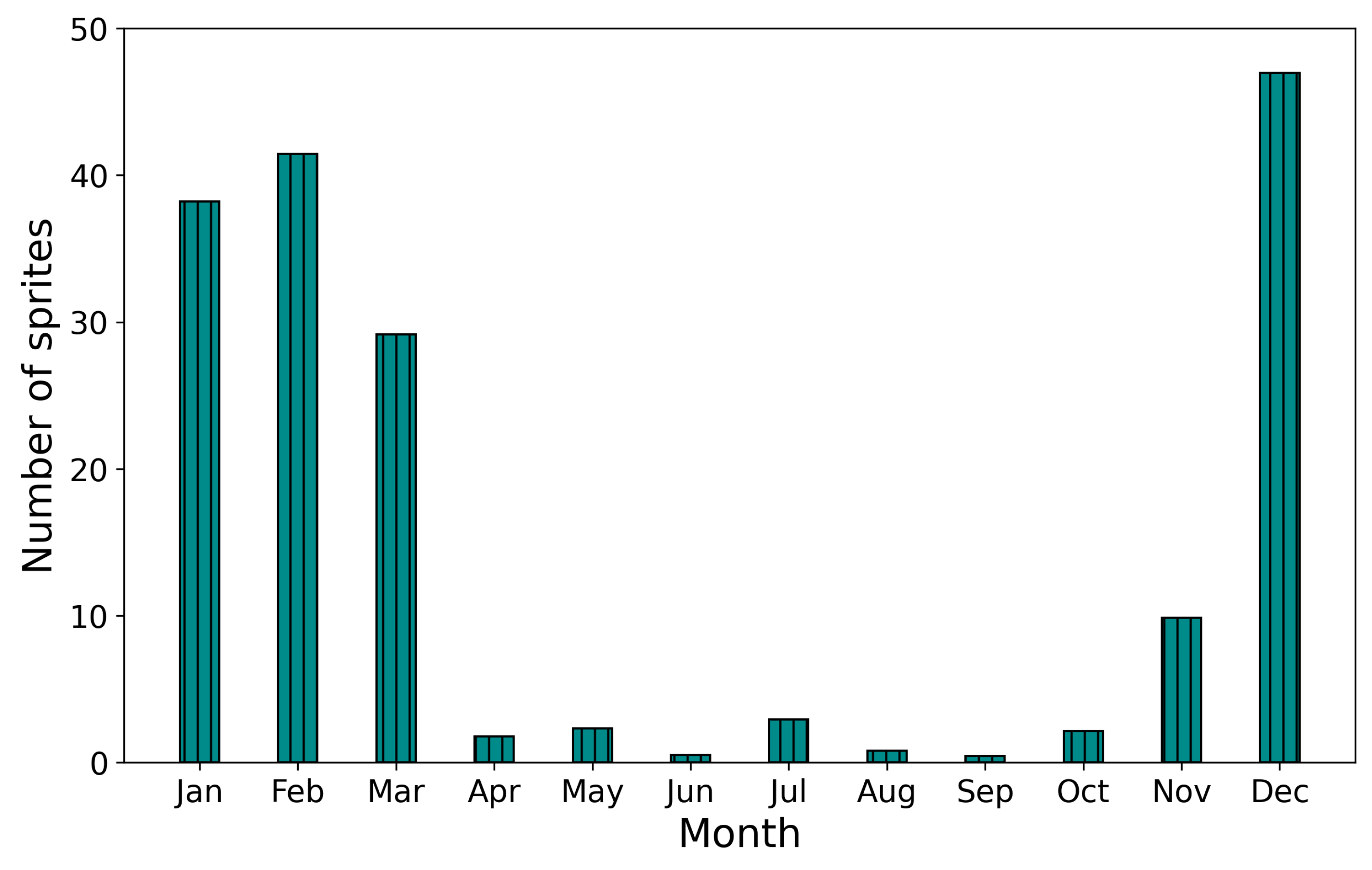
Figure 5 shows the monthly number of estimated sprites. As can be seen from the figure, December has the highest number of sprites. The estimated number of sprites from December to March is significantly higher than the rest of the months. This result is in agreement with the ASCA observations (Figure 1). The correlation coefficient between the observed and the estimated monthly averaged numbers of sprites is 0.86, showing a strong correlation (Table 1). A total of 537 sprites were observed by ASCA between September 2016 and February 2022, averaging 98 sprites per year. On the other hand, the number of estimated sprites is 176 yearly. Therefore, the number of estimated sprites is much higher than those observed.
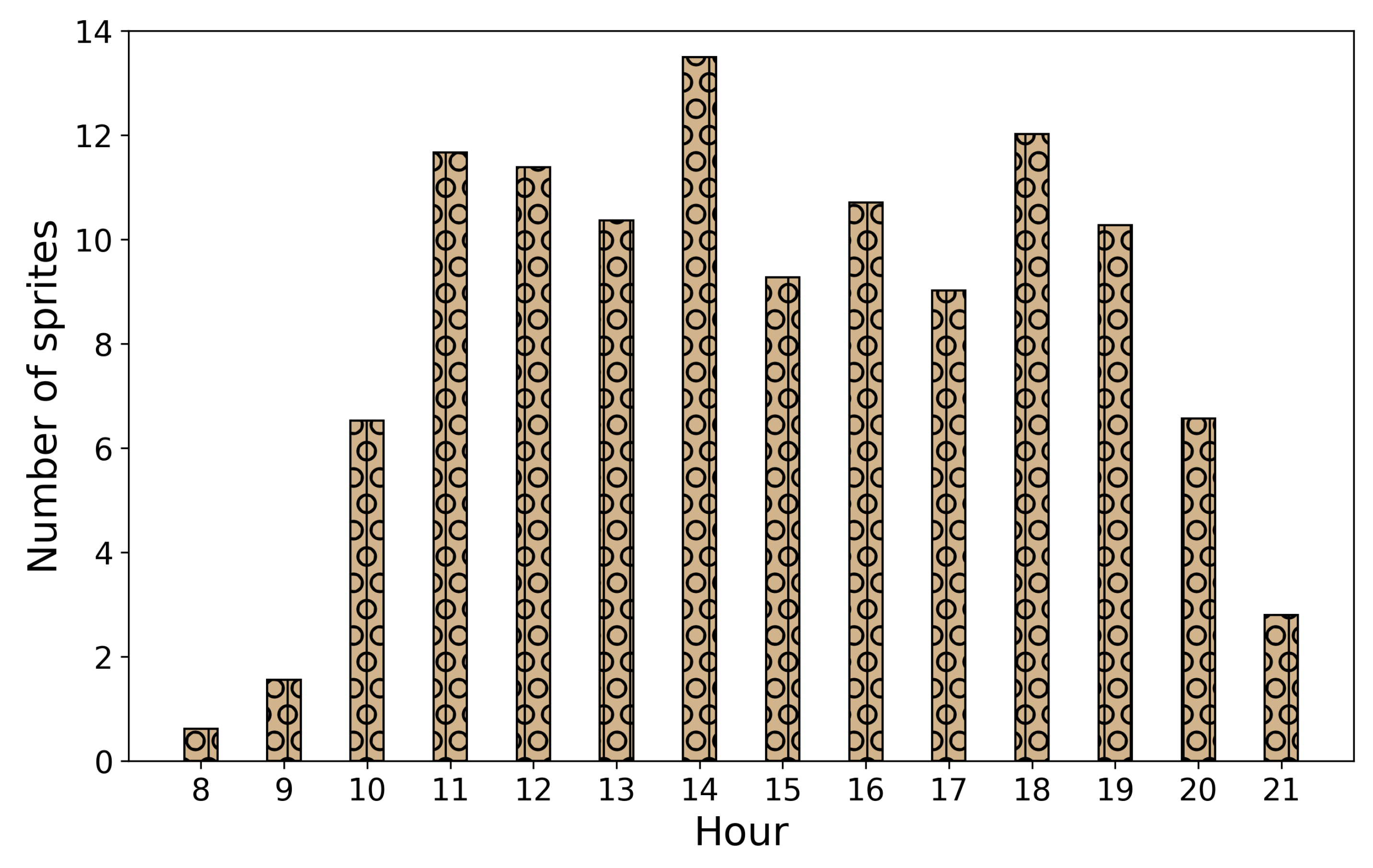
Figure 6 shows the hourly number of estimated sprites. There is a noticeable difference between the ASCA observation (Figure 2) and the estimate (Figure 6). The distribution of the hourly number of estimated sprites shows a flat trend. In contrast, the observed distribution peaks at 15–16 UT (Figure 2). The correlation coefficient between the hourly average number of observed sprites and the estimated numbers is considerably low (Table 1). Hence, the observed hourly distribution of sprites does not agree with the estimated distribution.
4. Improving the Sprite Number Estimation Model
As shown in Section 3, it is impossible to reproduce the hourly distribution of observed sprites when considering the iCMC and lightning polarity. Furthermore, the estimated number of sprites was much higher than the number observed. A significantly smaller number of sprites were observed at 8:00, 9:00, and 21:00 UTC, corresponding to dusk and dawn in Japan (Figure 2). at dusk and dawn is 100 times higher than midnight. A higher leads to a shorter , making the generation of sprites difficult. Therefore, fewer sprites tend to be observed at dusk and dawn. In addition, an air number density N and a thundercloud’s charge height also affect sprite generation. Therefore, we add these three factors into the model.
Electric fields are formed through the charging and discharging processes of thunderclouds. We assume that charges neutralized by lightning strokes have a spherically symmetric distribution, and their magnitudes are relatively small relative to the observation distance. Therefore, the electric field changes caused by the lightning strike can be considered equal to the electric field change caused by point charges in the thundercloud. is calculated as:
where x, y, z are the coordinates of the point charge Q; , , are the coordinates of a different observation site; and is a distance from the point charge to the observation site. When an observation site is directly above a thundercloud, a quasi-static electric field E is
where (=) is a charge moment change, r (=) is a distance from a charge in the thundercloud, (= [F/m]) is the vacuum permittivity, Q is an amount of charge discharged from the thundercloud, is the thundercloud’s charge height, and h is the altitude above the ground. The air breakdown electric field is proportional to the density of air and, thus, decays exponentially with altitude [29]. As such, can be described as
where (=) is the air number density at the ground level. Assuming that the time variation of electrical conductivity of air is negligible, we can derive the equation for [5] as:
where is determined in terms of Q, , N and [5].
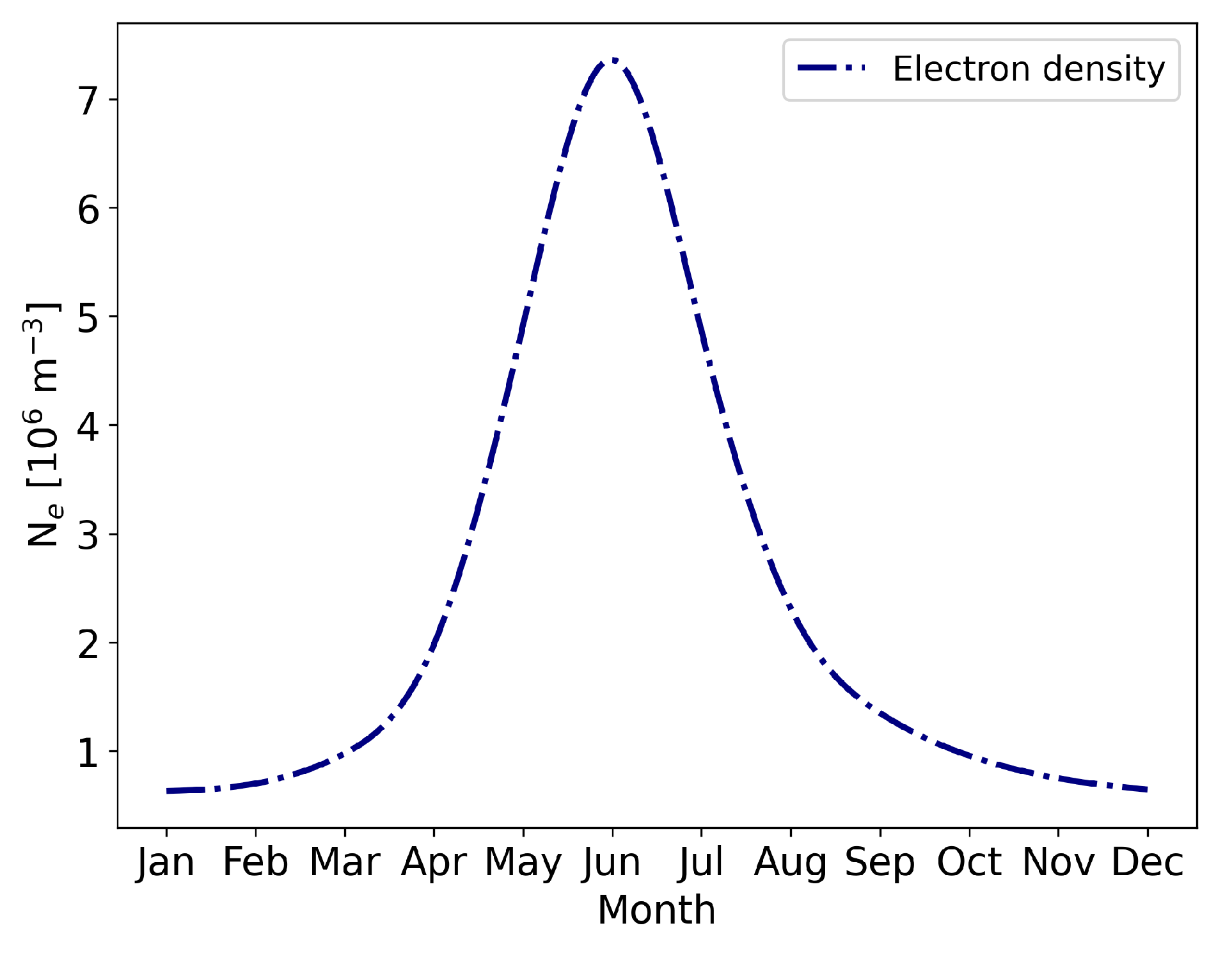
We use the International Reference Ionosphere (IRI) model https://ccmc.gsfc.nasa.gov/modelweb/models/iri2016_vitmo.php (accessed on 1 September 2022) [30] to study the seasonal and daily difference in . Given parameters such as date, latitude, and longitude, the IRI calculates in the ionosphere at a specific time and location. We set the height at 80 km—the same as the top height of sprites. As many sprites are detected around Wajima on the Sea of Japan side, the specified latitude and longitude are the location of the Wajima Meteorological Observatory ( N, E). We also use the observation data at C isotherm height from the Wajima Meteorological Observatory. Figure 7 shows the monthly average of during 2015 and 2020 at the time of 16:00 UTC. varies in different months, and is affected by seasonal changes. For instance, in July is 12 times higher than in January. Figure 8 shows the hourly average of in 2020 during the time between 8:00 and 21:00 UTC. The hourly distribution of is inversely correlated with the monthly distribution. For instance, at 8:00 UTC is 157 times higher than that at 16:00 UTC. Therefore, using this result, we can consider the change in to be caused by solar radiation.
Next, we use the Naval Research Laboratory Mass Spectrometer and Incoherent Scatter Radar Exosphere model (NRLMSISE-00) https://ccmc.gsfc.nasa.gov/modelweb/models/nrlmsise00.php (accessed on 1 September 2022) to investigate the monthly variation of N [31]. NRLMSISE-00 is a global standard atmospheric model based on Earth observations, modeling the temperature and number density of atmospheric components from the ground to space (∼1000 km). As the hourly variation of N is not apparent, we only consider the monthly variation of N, as shown in Figure 9.
According to Takahashi [32], Takahashi [33], charge separation in thunderclouds occurs actively at around C isotherm height. As the C isotherm height is similar to [34], can be estimated by examining the C isotherm height [35]. Using the meteorological data released by the Wajima Meteorological Observatory, we investigate the C isotherm height, and Figure 10 shows the monthly distribution of C isotherm height. Thunderclouds bring lightning strokes, accompanied by intense convection. In Japan, where seasonal winds prevail, thunderclouds occur both in summer and winter. The surface temperature from June to September is around 30 C. Due to surface heating, the C isotherm height exceeds 5.7 km. On the other hand, winter thunderclouds are formed when cold air from Siberia collides with water vapor produced by the Tsushima warm current. Therefore, the C isotherm height is approximately 2 km, as the sea surface or ground temperature is not as hot as in summer.
We substitute the monthly and N into Equations (5) and (6) to obtain E/ for different months. Then, the from 8:00 to 21:00 UTC is brought into Equation (7) to obtain at different times in different months. Conversely, as long as E/ and are determined, two CMC values, one from Equation (5) and another from Equation (7) (the CMC derived from ), are calculated. To be conservative, we pick the higher CMC as the CMC for each hour of each month. The lowest reliably recorded value of a CMC was 120 C·km [6]. Additionally, according to the statistical results of Hu et al. [6], the probability of triggering sprites is 90% when the +CG is over 1000 C·km within 6 ms. On the other hand, there is a 10% possibility of triggering a sprite when the CMC is less than 600 C·km. Above 600 C·km, the chance of generating sprites increases significantly [9]. Therefore, we assume the minimum threshold for sprite generation to be around 120 C·km. Considering that the probability of sprite generation increases remarkably when the threshold is above 600 C·km, we assume that the threshold is 600 C·km as the highest. Based on the above estimations, we set the thresholds for E/ and as 0.06 and 0.035 ms.
Assuming these thresholds for sprite generation, we obtain the CMC for each hour of each month, in order to determine when the criteria were met. Table 2 summarizes the thresholds. As can be seen from the table, the thresholds between 11:00 and 19:00 UTC are the same. This is because is small at night and, so, is large; thus, it is easy to meet the condition of . Therefore, the threshold value from 11:00 to 19:00 UTC is determined only by E/; furthermore, the daily changes in and N, calculated from E/, are not noticeable. On the other hand, as is high and is small at dusk and dawn (8:00, 9:00, 10:00, 20:00, and 21:00 UTC), a larger CMC is required to generate sprites. Note that our thresholds differ from those of Evtushenko et al. [16], who assumed 100 C·km for all months and hours.
The probability of sprite generation can be obtained by substituting the CMC values in Table 2 as iCMCs in Equation (3). Evtushenko et al. [16] added 300 to the threshold of 100 C·km for the parameter a of Equation (3). Similarly, we add 300 to the iCMCs in Table 2 to the parameter a. Figure 11 and Figure 12 show the results; in particular, Figure 11 gives a similar result to Figure 5. There is a strong correlation between the monthly number of estimated sprites and the observed sprite distribution (Table 1). The correlation coefficient between the estimated and the monthly average number of observed sprites is 0.85. On the other hand, Figure 12 differs from Figure 6. The estimated number of sprites at 8:00, 9:00, and 21:00 UTC are significantly lower than those at other hours. This trend is in agreement with the observations (Figure 2). The correlation coefficient between the estimated number and the hourly average number of observed sprites is 0.76, indicating a strong correlation.
Finally, we consider only the variation of to estimate the number of sprites. We take the monthly average values for and N as 4381 m and 3.6 × 10, respectively. The thresholds are E/ = 0.06 and = 0.035 ms. Figure 13 and Figure 14 show the number of estimated sprites. There is also a strong correlation between the estimated and observed sprite distributions (Table 1). Furthermore, the number of estimated sprites is 105, closer to the average of 98 sprites per year observed by ASCA. Therefore, we find that the variation of is important in understanding the monthly and hourly distribution of observed sprites.
5. Discussion and Conclusions
Although we found a good agreement in estimating the number of sprites, with respect to the observed data, we encountered several issues when using the WWLLN data. First, there is 25% uncertainty in the energy data of the WWLLN [36]. According to Evtushenko et al. [16], the lower bound of their estimate was reduced by 37%, whereas the upper bound was increased by 31%. Our estimate should have been affected by the same systematic uncertainty. Second, there is a sensitivity issue in the WWLLN data; for example, if the peak current is 50 kA, the detection efficiency of lightning is 80%. Therefore, our estimate could increase by 20%, considering the sensitivity. Third, the WWLLN detects intra-cloud discharges (ICs) with high peak current [37]; however, the ratio of ICs and CGs is not apparent in the WWLLN data, and we only consider CGs in our estimation. Therefore, this third point may also have affected our sprite estimation.
Another possible issue in our estimation is the data used to calculate the fraction of +CG. Although we used the result of Sugita and Matsui [25], the location was different from our observation site. In addition, the result was based on 2001–2010 data, in contrast to our observation period of 2016–2022. Therefore, further improvement of our calculation is needed to accurately estimate the number of sprites corresponding to our ASCA data.
In conclusion, the ASCA (located at Sagamihara, Japan) detected 537 sprites during continuous observations over a period of five and a half years. Notably, ASCA detected 303 sprites during the winter (56.4% of the total), and only 46 sprites in the summer (8.6% of the total). The daily distribution of sprites peaked at 15:00 and 16:00 UTC. Sprites were concentrated along the coast of the Sea of Japan, as well as being widely distributed on the Pacific side. Unlike other seasons, summer sprites were typically located over mainland Japan, and only four were detected over the sea near the coastline.
Using the WWLLN data from 2021, we estimated the number of sprites and compared the estimate with the observed ASCA results. The estimated monthly sprite distribution showed a strong correlation with the observed sprite distribution; however, the estimated hourly sprite distribution did not agree with the observation. Therefore, we updated the estimated model by considering the variation in , N, and , and found an excellent match to the observed distribution. Then, we investigated the model by only considering the variation in . Again, we observed a similar agreement with the data. Therefore, we can conclude that the energy of lightning, the monthly ratio of +CG, and the hourly variation of are the crucial parameters for the generation of sprites.
Author Contributions
Conceptualization, M.D. and T.S.; data curation, M.D. and T.S.; funding acquisition and project administration, M.D. and T.S.; investigation, M.D. and T.S.; validation, M.D. and T.S.; visualization, M.D. and T.S.; supervision, M.D. and T.S.; writing—original draft preparation, M.D.; writing—review and editing, M.D. and T.S. All authors have read and agreed to the published version of the manuscript.
Funding
This work was supported by JST SPRING, Grant Number JPMJSP2103.
Institutional Review Board Statement
Not applicable.
Informed Consent Statement
Not applicable.
Data Availability Statement
Not applicable.
Acknowledgments
We would like to to thank the anonymous referees for comments and suggestions that materially improved the paper. We also would like to thank the World Wide Lightning Location Network http://wwlln.net (accessed on 1 September 2022), a collaboration among over 50 universities and institutions, for providing the lightning location data used in this paper. This work was supported by JST SPRING, Grant Number JPMJSP2103.
Conflicts of Interest
The authors declare no conflict of interest.
Abbreviations
The following abbreviations are used in this manuscript:
| ASCA | Aoyama Gakuin University Sprite Camera |
| CMC | Charge moment change |
| EUCLID | European Cooperation for Lightning Detection |
| JLDN | Japanese Lightning Detection Network |
| iCMC | Impulse charge moment change |
| IRI | International Reference Ionosphere |
| NLDN | National Lightning Detection Network |
| NRLMSISE | Naval Research Laboratory Mass Spectrometer and Incoherent Scatter Radar Exosphere |
| +CG | Positive cloud-to-ground discharge |
| URSI | International Union of Radio Science |
| WWLLN | World Wide Lightning Location Network |
References
- Pasko, V.P.; Stanley, M.A.; Mathews, J.D.; Inan, U.S.; Wood, T.G. Electrical discharge from a thundercloud top to the lower ionosphere. Nature 2002, 416, 152–154. [Google Scholar] [CrossRef] [PubMed]
- Chou, J.; Kuo, C.L.; Tsai, L.; Chen, A.; Su, H.; Hsu, R.; Cummer, S.; Li, J.; Frey, H.; Mende, S.; et al. Gigantic jets with negative and positive polarity streamers. J. Geophys. Res. Space Phys. 2010, 115, A00E45. [Google Scholar] [CrossRef] [Green Version]
- Soula, S.; van der Velde, O.; Montanya, J.; Huet, P.; Barthe, C.; Bór, J. Gigantic jets produced by an isolated tropical thunderstorm near Réunion Island. J. Geophys. Res. 2011, 116, D19103. [Google Scholar] [CrossRef] [Green Version]
- Pasko, V.P.; Inan, U.S.; Taranenko, Y.N.; Bell, T.F. Heating, ionization and upward discharges in the mesosphere, due to intense quasi-electrostatic thundercloud fields. Geophys. Res. Lett. 1995, 22, 365–368. [Google Scholar] [CrossRef]
- Pasko, V.; Inan, U.; Bell, T.; Taranenko, Y.N. Sprites produced by quasi-electrostatic heating and ionization in the lower ionosphere. J. Geophys. Res. Space Phys. 1997, 102, 4529–4561. [Google Scholar] [CrossRef]
- Hu, W.; Cummer, S.A.; Lyons, W.A.; Nelson, T.E. Lightning charge moment changes for the initiation of sprites. Geophys. Res. Lett. 2002, 29, 120–121. [Google Scholar] [CrossRef] [Green Version]
- Hobara, Y.; Iwasaki, N.; Hayashida, T.; Hayakawa, M.; Ohta, K.; Fukunishi, H. Interrelation between ELF transients and ionospheric disturbances in association with sprites and elves. Geophys. Res. Lett. 2001, 28, 935–938. [Google Scholar] [CrossRef]
- Hayakawa, M.; Nakamura, T.; Hobara, Y.; Williams, E. Observation of sprites over the Sea of Japan and conditions for lightning-induced sprites in winter. J. Geophys. Res. 2004, 109, A01312. [Google Scholar] [CrossRef]
- Cummer, S.A.; Lyons, W.A. Implications of lightning charge moment changes for sprite initiation. J. Geophys. Res. Space Phys. 2005, 110, A04304. [Google Scholar] [CrossRef] [Green Version]
- Qin, J.; Celestin, S.; Pasko, V.P. Dependence of positive and negative sprite morphology on lightning characteristics and upper atmospheric ambient conditions. J. Geophys. Res. Space Phys. 2013, 118, 2623–2638. [Google Scholar] [CrossRef]
- Asano, T.; Hayakawa, M.; Cho, M.; Suzuki, T. Computer simulations on the initiation and morphological difference of Japan winter and summer sprites. J. Geophys. Res. Space Phys. 2008, 113, A02308. [Google Scholar] [CrossRef] [Green Version]
- Nakamura, T.; Hayakawa, M. Characteristics of Mesopheric Sprites in the Hokuriku Area and their Causative Lightning Discharges. IEEJ Trans. Power Energy 2004, 124, 1012–1020. [Google Scholar] [CrossRef] [Green Version]
- Suzuki, T.; Hayakawa, M.; Matsudo, Y.; Michimoto, K. How do winter thundercloud systems generate sprite-inducing lightning in the Hokuriku area of Japan? Geophys. Res. Lett. 2006, 33, L10806. [Google Scholar] [CrossRef]
- Brook, M.; Nakano, M.; Krehbiel, P.; Takeuti, T. The electrical structure of the hokuriku winter thunderstorms. J. Geophys. Res. 1982, 87, 1207. [Google Scholar] [CrossRef]
- Stanley, M.; Brook, M.; Krehbiel, P.; Cummer, S.A. Detection of daytime sprites via a unique sprite ELF signature. Geophys. Res. Lett. 2000, 27, 871–874. [Google Scholar] [CrossRef] [Green Version]
- Evtushenko, A.; Ilin, N.; Svechnikova, E. Parameterization and global distribution of sprites based on the WWLLN data. Atmos. Res. 2022, 276, 106272. [Google Scholar] [CrossRef]
- Abarca, S.F.; Corbosiero, K.L.; Galarneau, T.J., Jr. An evaluation of the Worldwide Lightning Location Network (WWLLN) using the National Lightning Detection Network (NLDN) as ground truth. J. Geophys. Res. 2010, 115, D18206. [Google Scholar] [CrossRef]
- Connaughton, V.; Briggs, M.; Holzworth, R.; Hutchins, M.; Fishman, G.; Wilson-Hodge, C.; Chaplin, V.; Bhat, P.; Greiner, J.; Von Kienlin, A.; et al. Associations between Fermi Gamma-ray Burst Monitor terrestrial gamma ray flashes and sferics from the World Wide Lightning Location Network. J. Geophys. Res. Space Phys. 2010, 115, A12307. [Google Scholar] [CrossRef]
- Holzworth, R.; McCarthy, M.; Brundell, J.; Jacobson, A.; Rodger, C. Global Distribution of Superbolts. J. Geophys. Res. Atmos. 2019, 124, 9996–10005. [Google Scholar] [CrossRef] [Green Version]
- Hutchins, M.L.; Holzworth, R.H.; Rodger, C.J.; Brundell, J.B. Far-Field Power of Lightning Strokes as Measured by the World Wide Lightning Location Network. J. Atmos. Ocean. Technol. 2012, 29, 1102–1110. [Google Scholar] [CrossRef]
- Lu, G.; Cummer, S.A.; Blakeslee, R.J.; Weiss, S.; Beasley, W.H. Lightning morphology and impulse charge moment change of high peak current negative strokes. J. Geophys. Res. Atmos. 2012, 117, D04212. [Google Scholar] [CrossRef] [Green Version]
- Cummer, S.A.; Lyons, W.A.; Stanley, M.A. Three years of lightning impulse charge moment change measurements in the United States. J. Geophys. Res. Atmos. 2013, 118, 5176–5189. [Google Scholar] [CrossRef]
- Lu, G.; Cummer, S.A.; Chen, A.B.; Lyu, F.; Li, D.; Liu, F.; Hsu, R.R.; Su, H.T. Analysis of lightning strokes associated with sprites observed by ISUAL in the vicinity of North America. Terr. Atmos. Ocean. Sci. 2017, 28, 583–595. [Google Scholar] [CrossRef] [Green Version]
- Zajac, B.A.; Rutledge, S.A. Cloud-to-ground lightning activity in the contiguous United States from 1995 to 1999. Mon. Weather. Rev. 2001, 129, 999–1019. [Google Scholar] [CrossRef]
- Sugita, A.; Matsui, M. Lightning characteristics in Japan observed by the JLDN from 2001 to 2010. In Proceedings of the 22nd International Lightning Detection Conference, Broomfield, CO, USA, 2–5 April 2012; pp. 2–3. [Google Scholar]
- Qin, J.; Celestin, S.; Pasko, V.P. Minimum charge moment change in positive and negative cloud to ground lightning discharges producing sprites. Geophys. Res. Lett. 2012, 39, L22801. [Google Scholar] [CrossRef]
- Lu, G.; Cummer, S.A.; Li, J.; Zigoneanu, L.; Lyons, W.A.; Stanley, M.A.; Rison, W.; Krehbiel, P.R.; Edens, H.E.; Thomas, R.J.; et al. Coordinated observations of sprites and in-cloud lightning flash structure. J. Geophys. Res. Atmos. 2013, 118, 6607–6632. [Google Scholar] [CrossRef] [Green Version]
- Chen, A.B.C.; Chen, H.; Chuang, C.W.; Cummer, S.A.; Lu, G.; Fang, H.K.; Su, H.T.; Hsu, R.R. On negative Sprites and the Polarity Paradox. Geophys. Res. Lett. 2019, 46, 9370–9378. [Google Scholar] [CrossRef]
- Papadopoulos, K.; Milikh, G.; Gurevich, A.; Drobot, A.; Shanny, R. Ionization rates for atmospheric and ionospheric breakdown. J. Geophys. Res. 1993, 98, 17593. [Google Scholar] [CrossRef]
- Bilitza, D.; Altadill, D.; Zhang, Y.; Mertens, C.; Truhlik, V.; Richards, P.; McKinnell, L.A.; Reinisch, B. The International Reference Ionosphere 2012—A model of international collaboration. J. Space Weather Space Clim. 2014, 4, A07. [Google Scholar] [CrossRef]
- Picone, J.; Hedin, A.; Drob, D.P.; Aikin, A. NRLMSISE-00 empirical model of the atmosphere: Statistical comparisons and scientific issues. J. Geophys. Res. Space Phys. 2002, 107, 1468. [Google Scholar] [CrossRef]
- Takahashi, T. Riming electrification as a charge generation mechanism in thunderstorms. J. Atmos. Sci. 1978, 35, 1536–1548. [Google Scholar] [CrossRef]
- Takahashi, T. Thunderstorm electrification—A numerical study. J. Atmos. Sci. 1984, 41, 2541–2558. [Google Scholar] [CrossRef]
- Michimoto, K. A Study of Radar Echoes and their Relation to Lightning Discharges of Thunderclouds in the Hokuriku District. J. Meteorol. Soc. Japan Ser. II 1993, 71, 195–204. [Google Scholar] [CrossRef] [Green Version]
- Myokei, K.; Matsudo, Y.; Asano, T.; Sekiguchi, M.; Suzuki, T.; Hobara, Y.; Hayakawa, M. Morphology of winter sprites in the Hokuriku area of Japan: Monthly variation and dependence on air temperature. J. Atmos. Electr. 2009, 29, 23–34. [Google Scholar] [CrossRef] [Green Version]
- Hutchins, M.; Holzworth, R.; Brundell, J.; Rodger, C. Relative detection efficiency of the World Wide Lightning Location Network. Radio Sci. 2012, 47, RS6005. [Google Scholar] [CrossRef]
- Fan, P.; Zheng, D.; Zhang, Y.; Gu, S.; Zhang, W.; Yao, W.; Yan, B.; Xu, Y. A Performance Evaluation of the World Wide Lightning Location Network (WWLLN) over the Tibetan Plateau. J. Atmos. Ocean. Technol. 2018, 35, 927–939. [Google Scholar] [CrossRef]
Figure 1.
Distribution of the monthly number of sprites observed by ASCA. The red bars show the monthly averaged number of observed sprites from September 2016 to February 2022, and the blue bars show the monthly number of observed sprites in 2021.
Figure 1.
Distribution of the monthly number of sprites observed by ASCA. The red bars show the monthly averaged number of observed sprites from September 2016 to February 2022, and the blue bars show the monthly number of observed sprites in 2021.

Figure 2.
Distribution of the hourly number of sprites observed by ASCA. The yellow bars show the hourly averaged number of observed sprites from September 2016 to February 2022, and the green bars show the hourly number of observed sprites in 2021. 8:00 and 21:00 UTC correspond to 17:00 and 6:00 JST.

Figure 3.
Location map of 537 sprites from September 2016 to February 2022 in different seasons observed by ASCA. Spring, summer, autumn, and winter are represented by green triangles, red dots, light blue diamonds, and blue dots, respectively. Lightning distribution within 100 km from the detected sprites is shown as a brown contour. The background map is provided by Geospatial Information Authority of Japan.

Figure 4.
Field of view of the three ASCA cameras. Spring, summer, autumn, and winter are represented by green triangles, red dots, light blue diamonds, and blue dots, respectively.
Figure 4.
Field of view of the three ASCA cameras. Spring, summer, autumn, and winter are represented by green triangles, red dots, light blue diamonds, and blue dots, respectively.

Figure 5.
Estimated monthly distribution of sprites in case A (see caption of Table 1 for an explanation of the three different cases).
Figure 5.
Estimated monthly distribution of sprites in case A (see caption of Table 1 for an explanation of the three different cases).

Figure 6.
Estimated hourly distribution of sprites in case A (see caption of Table 1 for an explanation of the three different cases).
Figure 6.
Estimated hourly distribution of sprites in case A (see caption of Table 1 for an explanation of the three different cases).

Figure 7.
Monthly variation of electron number density at a height of 80 km.

Figure 8.
Hourly variation of electron number density at a height of 80 km.

Figure 9.
Monthly variation of air number density N at a height of 80 km.

Figure 10.
Monthly −10 °C isotherm height distribution at the Wajima Meteorological Observatory.

Figure 11.
Estimated monthly number of sprites in case B (see caption of Table 1 for an explanation of the three different cases).
Figure 11.
Estimated monthly number of sprites in case B (see caption of Table 1 for an explanation of the three different cases).

Figure 12.
Estimated hourly number of sprites in case B (see caption of Table 1 for an explanation of the three different cases).
Figure 12.
Estimated hourly number of sprites in case B (see caption of Table 1 for an explanation of the three different cases).

Figure 13.
Estimated monthly number of sprites in case C (see caption of Table 1 for an explanation of the three different cases).
Figure 13.
Estimated monthly number of sprites in case C (see caption of Table 1 for an explanation of the three different cases).

Figure 14.
Estimated hourly number of sprites in case C (see caption of Table 1 for an explanation of the three different cases).
Figure 14.
Estimated hourly number of sprites in case C (see caption of Table 1 for an explanation of the three different cases).


Table 1.
Correlation coefficients between the estimated and the observed number of sprites. The columns and are the coefficients using the monthly averaged number of observed sprites in 2016–2022 and 2021 alone, respectively. The columns and are the coefficients using the hourly averaged number of observed sprites in 2016–2022 and 2021 alone, respectively. “Case A” is the case where the estimated number of sprites is derived without any condition. “Case B” is the case where the number of sprites is estimated considering temporal variation of , , and N. “Case C” is the case where the number of sprites is estimated considering only temporal variation of .
| Case A: no condition | 0.86 | 0.73 | 0.16 | 0.25 |
| Case B: , and N | 0.85 | 0.72 | 0.76 | 0.64 |
| Case C: | 0.83 | 0.70 | 0.77 | 0.59 |
Table 2.
CMC thresholds for estimating the number of sprites. The unit is C·km.
| UTC | Jan | Feb | Mar | Apr | May | Jun | Jul | Aug | Sep | Oct | Nov | Dec |
|---|---|---|---|---|---|---|---|---|---|---|---|---|
| 8:00 | 620.14 | 588.16 | 514.62 | 418.11 | 345.20 | 311.20 | 308.57 | 348.48 | 418.9 | 509.13 | 570.07 | 608.81 |
| 9:00 | 447.12 | 420.41 | 368.00 | 302.63 | 257.69 | 230.52 | 228.07 | 252.82 | 303.55 | 360.84 | 407.19 | 439.40 |
| 10:00 | 192.46 | 184.32 | 166.75 | 143.35 | 131.27 | 132.55 | 127.45 | 122.99 | 139.63 | 163.12 | 178.39 | 190.58 |
| 11:00–19:00 | 118.58 | 120.12 | 123.62 | 127.42 | 131.27 | 132.55 | 127.45 | 116.16 | 115.35 | 113.69 | 112.46 | 113.82 |
| 20:00 | 196.34 | 188.46 | 169.62 | 143.35 | 131.27 | 132.55 | 127.45 | 122.99 | 145.7 | 163.12 | 182.27 | 193.23 |
| 21:00 | 451.01 | 424.56 | 373.75 | 306.61 | 257.69 | 230.52 | 228.07 | 259.65 | 303.55 | 365.78 | 414.95 | 444.70 |
Disclaimer/Publisher’s Note: The statements, opinions and data contained in all publications are solely those of the individual author(s) and contributor(s) and not of MDPI and/or the editor(s). MDPI and/or the editor(s) disclaim responsibility for any injury to people or property resulting from any ideas, methods, instructions or products referred to in the content. |
© 2023 by the authors. Licensee MDPI, Basel, Switzerland. This article is an open access article distributed under the terms and conditions of the Creative Commons Attribution (CC BY) license (https://creativecommons.org/licenses/by/4.0/).
Share and Cite
MDPI and ACS Style
Duan, M.; Sakamoto, T. Estimation of the Number of Sprites Observed over Japan in 5.5 Years Using Lightning Data. Atmosphere 2023, 14, 105. https://doi.org/10.3390/atmos14010105
AMA Style
Duan M, Sakamoto T. Estimation of the Number of Sprites Observed over Japan in 5.5 Years Using Lightning Data. Atmosphere. 2023; 14(1):105. https://doi.org/10.3390/atmos14010105
Chicago/Turabian StyleDuan, Maomao, and Takanori Sakamoto. 2023. "Estimation of the Number of Sprites Observed over Japan in 5.5 Years Using Lightning Data" Atmosphere 14, no. 1: 105. https://doi.org/10.3390/atmos14010105
Note that from the first issue of 2016, this journal uses article numbers instead of page numbers. See further details here.