Article

Characterization of Particle Number Setups for Measuring Brake Particle Emissions and Comparison with Exhaust Setups

1
European Commission, Joint Research Centre (JRC), 21027 Ispra, Italy
2
Corning GmbH, D-65189 Wiesbaden, Germany
3
AVL List GmbH, 8010 Graz, Austria
4
HORIBA Europe GmbH, D-61440 Oberursel, Germany
5
TSI Inc., Shoreview, MN 55126, USA
6
AIP GmbH & Co. KG, D-87490 Haldenwang, Germany
7
Dekati Ltd., FI-36240 Kangasala, Finland
8
Airmodus Oy, FI-00560 Helsinki, Finland
9
Singularity Scientific Consulting Services, LLC, Whitmore Lake, MI 48189, USA
10
Link Engineering Co., Plymouth, MI 48170, USA
*
Author to whom correspondence should be addressed.
Atmosphere 2023, 14(1), 103; https://doi.org/10.3390/atmos14010103
Submission received: 1 December 2022 / Revised: 21 December 2022 / Accepted: 30 December 2022 / Published: 3 January 2023
(This article belongs to the Special Issue Brake Wear Particulate Matter and Mitigation Strategies)

Abstract

:
The stringency of vehicle exhaust emissions regulations resulted in a significant decrease in exhaust particulate matter (PM) emissions over the years. Non-exhaust particles (i.e., from brakes and tyres) account for almost half or more of road transport-induced ambient PM. Even with the internal combustion engine ban in 2035, electrified vehicles will still emit PM from brake and tyre wear. Consequently, non-exhaust PM emissions cannot decrease significantly without any regulatory measures. Because independent research carried out under different methods is not readily comparable, a Global Technical Regulation (GTR), which sets the procedures and boundaries of testing brake wear particle emissions, is currently under development. This overview describes the particle number (PN) measurement setup based on the well-known exhaust emissions PN methodology. We provide the technical requirements and the expected maximum losses. In addition, we estimate the effect of particle losses on the differences between different setups for typical size distributions observed during brake testing. Finally, we compare brake testing PN specifications to those of exhaust PN.

1. Introduction

Air pollution is considered the single most significant environmental health risk in Europe. Air pollution can cause cardiovascular and respiratory diseases that lead to the loss of healthy years of life and, in the most severe cases, to premature death [1]. Particulate matter (PM) is the most harmful component of air pollutants [2]. Globally, more than 50% of the population lives in urban areas with poor air quality [3]. In 2020 in the European Union, 96% of the urban population was exposed to levels of fine particulate matter above the health-based guideline level set by the World Health Organization (WHO) [4]. The contribution of vehicle emissions to ambient PM concentrations is around 10% or higher in cities or industrial areas [4,5,6,7,8]. Other sources such as shipping or residential heating are important depending on the area [9,10,11,12,13,14].
Worldwide vehicle emission regulations have controlled the PM since the 1990s [15]. The primary methodology is collecting PM from dilute exhaust gas on a filter and weighing it after a test [16]. The test typically includes a vehicle on a chassis dynamometer or an engine directly connected to a dynamometer following a prescribed torque/speed cycle. The methodology reached its sensitivity limits with the introduction of Diesel particulate filters (DPFs) to the aftertreatment systems of the engines and vehicles. A big step was the shift to a different metric. The introduction of the particle number (PN) method initially took place in Europe in 2011 and later in other regions in Asia [17]. The methodology was based on the work of the Particle Measurement Programme (PMP) group, which began its work in the early 2000s. In a nutshell, it includes thermal pre-treatment of the aerosol to remove volatile particles and to count the remaining particles larger than 23 nm. The sample was taken from a dilution tunnel where the entirety of the vehicle exhaust gas was mixed and cooled [17].
The introduction of more stringent regulations on exhaust emissions resulted in significant decreases in ambient gaseous pollutants in many regions worldwide. However, recently published data indicate that decreases in PM have not followed this trend [18]. As exhaust PM emissions from on-road vehicles have decreased over time, non-exhaust PM emissions’ relative contribution to ambient PM concentrations has increased. As a result, brake- and tyre-wear PM emissions’ impact on urban areas and nearby communities has become more concerning. According to many researchers, non-exhaust PM emissions’ contribution already accounts for almost half or more of all road transport-induced ambient PM concentrations [19,20,21]. Current models predict that airborne brake- and tyre-wear PM emissions will increase with the vehicle distance travelled. However, these projections still do not account for new vehicle technologies such as “zero emissions” and hybrid vehicles, which use some form of non-friction braking (regenerative braking) and low-rolling resistance tires. In any case, the contribution of non-exhaust PM to air pollution remains a concern because fully electric vehicles also emit these particles in relatively large numbers [22].
Researchers have reported that braking events can result in high PM mass emissions [23]. Light-duty vehicle (LDV) PM with aerodynamic diameter smaller than 10 μm (PM10) emission factors varying between 1–15 mg/km per vehicle have been reported in the literature following different methodologies (e.g., laboratory and on-road testing with different setups) [24,25,26,27]. However, recent results indicate that specific vehicle-brake configurations may emit up to 25–30 mg/km per vehicle, tested with a procedure following the draft specifications of the brakes GTR [28]. The per-vehicle emission factors are typically estimated by multiplying the brake corner emissions by three. This is a commonly accepted way within the industry to calculate overall vehicle emissions using the emission result from a brake corner and relies on the fact that brake power is usually split in front/rear by 70–30% [29]. The Euro 7 pollutants regulation preparation used a fleet-based PM10 emission factor of 12 mg/km per vehicle for LDV up to 3.5 t. This value was adopted in the recently published impact assessment to propose limiting brake PM10 of LDV to 3.5t to 7 mg/km per vehicle. PM2.5 emission factors are approximately 25–40% of PM10 [28,30]. Regarding particle number emissions, the results are more diverse [24]. Emission levels varying between 109–1013 #/km have been reported in the literature [25,30,31,32]. This range of values highlights the critical contribution of volatile particles emitted sometimes by brakes that can increase the emissions by orders of magnitude [33]. Studies link the exceedance of a certain temperature threshold with the release of a separate volatile nucleation mode peaking at 10–30 nm [31,34,35,36,37]. However, this temperature threshold is not well-defined since it depends upon various parameters (e.g., the brake system type, the brake components’ thermal masses, bedding condition, and the temperature measurement method) [30,38]. PN size distribution typically exhibits a peak around 1–2 μm, contributing to the mass [29,38,39,40,41]. Sometimes a peak around 100–300 nm is also reported [29,41,42].
The results reported in the literature are not readily comparable due to different approaches/methodologies, brake dynamometer setups, testing cycles, and measurement instrumentation [43]. A recent study discusses the most common configurations and their advantages and disadvantages [25]. To overcome this problem, the Working Party on Energy and Pollution (GRPE) mandated the PMP group to develop a standard methodology for sampling and measuring brake wear particle emissions from LDV up to 3.5 t. The overall process included several steps, with the most important being the development of a new braking cycle representative of real-world conditions, the definition of an appropriate setup for sampling brake wear particles, the definition of the appropriate instrumentation for measuring brake wear particle emissions, and the validation and further refinement of the overall methodology following the organization of an Inter-Laboratory Study (ILS). These steps have been described in detail elsewhere [44]. Additionally, in 2021, the GRPE mandated the PMP group to develop a Global Technical Regulation (GTR) governing the measurement of brake wear particle emissions from LDV up to 3.5 t. Larger vehicles (heavy-duty buses and trucks) will be addressed in the second phase as the braking mechanism differs from that of LDVs and more data are required for understanding the share of friction brakes to real-world brake emissions of these vehicles (e.g., contribution of engine and regenerative braking, representative test cycle).
Based on this background, the PMP developed the first set of recommendations for sampling and measuring brake particle emissions and organized an ILS to assess and further refine the proposed methodology for determining brake PM and PN emissions. The recommendations for measuring brake PN emissions heavily relied on the existing regulatory framework for exhaust emissions. The ILS study concluded that the proposed method is suitable for measuring solid brake PN emissions. Some minor refinements were introduced to the final proposal to consider the specific design needs of the brake emissions measurement setup. In addition to the solid PN (SPN) emissions, the ILS explored the feasibility of sampling and measuring total PN emissions (TPN) (i.e., solids and volatile particles). The ILS campaign confirmed literature findings concerning brake PN concentrations. In some cases, the brake released a volatile particle fraction, resulting in PN concentrations 1–2 orders of magnitude higher than the SPN measurements [33]. More profound research on brakes for this fraction is lacking compared to exhaust volatile nucleation mode [45]. The UN GTR proposed including TPN measurement specifications to generate more data that can be collected and used to improve understanding of the phenomenon and its possible occurrence in real-world situations.
The current paper presents the proposed setup for measuring SPN and TPN within the UN GTR for brake wear particle emissions from LDV up to 3.5 t. Additionally, this paper discusses PN penetration factors and the impact of the design criteria. The main aim of the paper is to evaluate the proposed methodology and estimate differences that could be found between different facilities. Additionally, we aim to provide guidance to testing facilities in setting up their measurement system in accordance with the GTR. Lastly, the paper provides a detailed comparison with the setup used in exhaust regulation.

2. Materials and Methods

2.1. Overview of Setups

The brake wear emissions GTR provides a methodology for measuring particulate emissions from brakes used on LDV up to 3.5 t. The tests use a brake dynamometer executing a prescribed cycle, namely the worldwide light vehicles test procedure brake cycle (WLTP-Brake cycle) [46]. The brake is installed in an enclosure to prevent untreated air from entering and contaminating the air flowing around the brake assembly. The climatic conditioning system circulates filtered and conditioned air while sampling from a tunnel connected to the brake enclosure. The setup uses separate sampling probes for PM and PN emission measurements. The PM sampling separates particles with an aerodynamic diameter of up to 10 μm (PM10) and up to 2.5 μm (PM2.5). The PN measurement can be performed either with separate sampling probes or through the same sampling probe using an appropriate flow-splitting device. The PN measurement covers particle sizes from approximately 10 nm to 10 μm depending on the cut-off size of the pre-classifier. Depending on the thermal pre-treatment of the individual aerosol streams, the PN setup counts SPN and TPN (abbreviated SPN10 and TPN10, respectively, based on the lower cut-off diameter of 10 nm). Figure 1 summarizes the primary components of the PN setup, including the following:
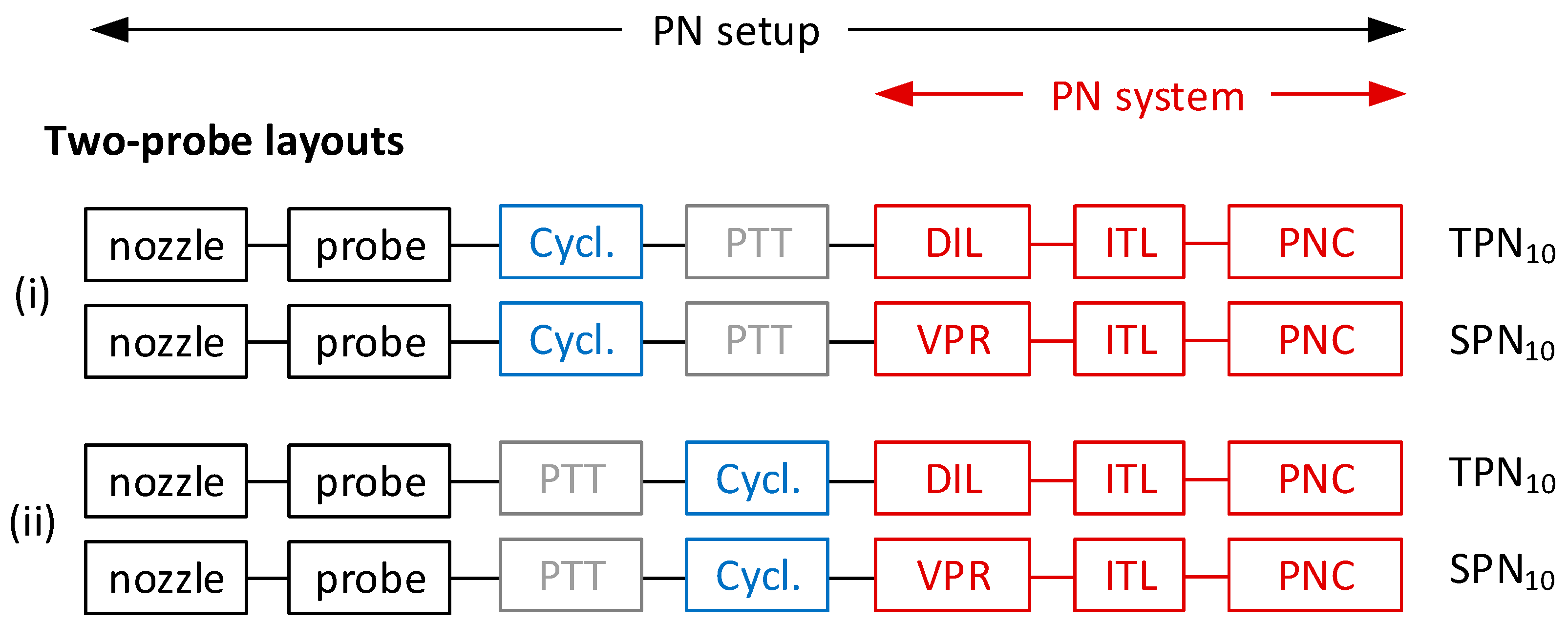
  • Probe(s) to extract the diluted sample. The setup can use a single probe followed by a flow-splitting device. Alternatively, two probes can sample TPN10 and SPN10 separately. In such a case, the setup consists of two different PN layouts.
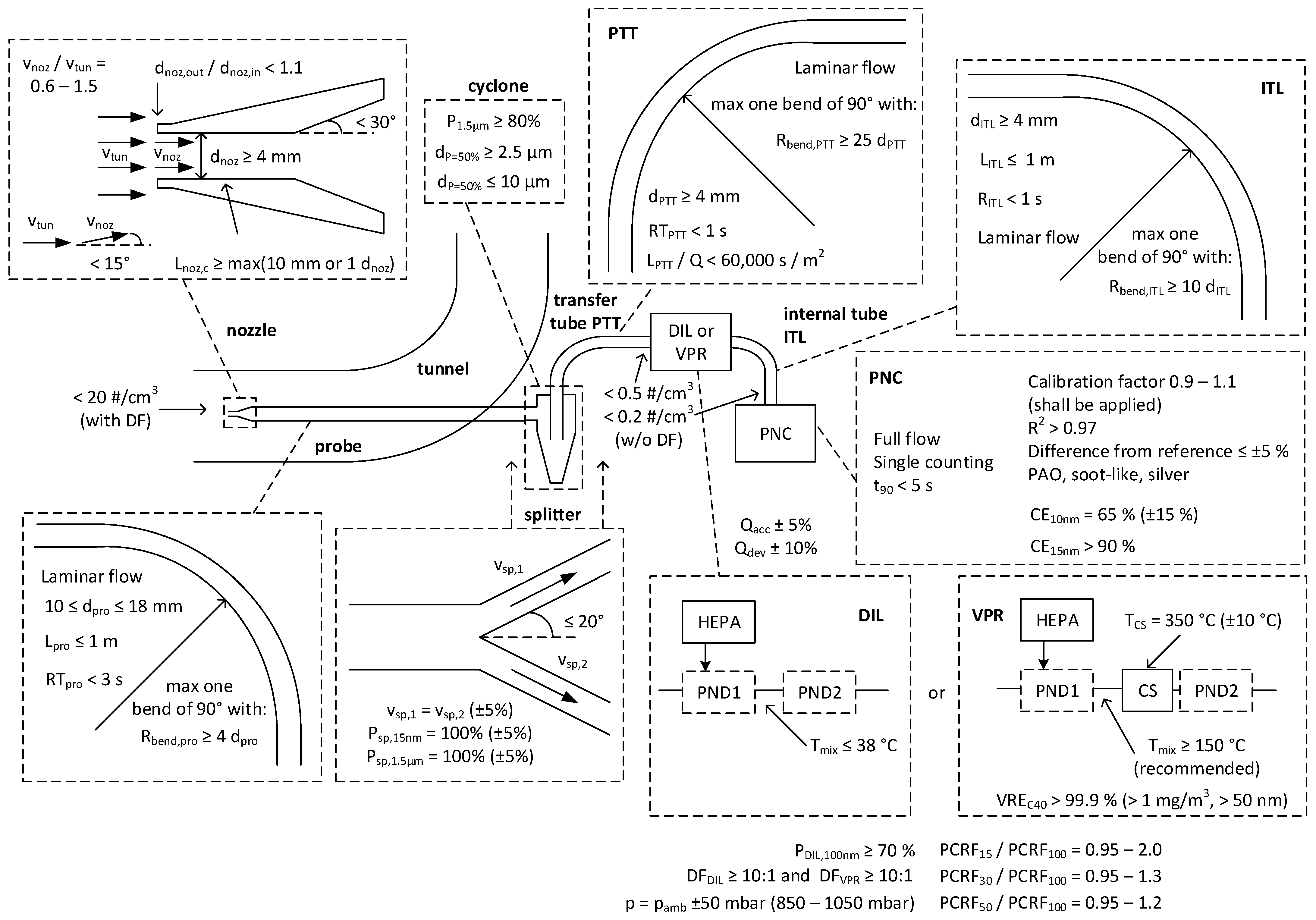
  • Nozzle(s) fitted to the probe’s end to achieve isokinetic sampling. The nozzle(s) must have its axis parallel to the dilution tunnel ensuring that the aspiration angle does not exceed 15°.
  • Cyclonic separator(s) to remove particles larger than 2.5 μm, which typically do not contribute to the PN concentration but might contaminate the PN system(s). The system can use a cyclonic separator with a higher cut-off point of up to 10 μm. Two cyclonic separators must be applied when using different probes for sampling TPN10 and SPN10 or when the cyclonic separators are downstream of the flow-splitting device. The cyclonic separator(s) must be mounted directly at the sampling probe’s outlet or the PN system’s inlet.
  • A flow splitter (optionally) is necessary when two PN systems are sampling from the same probe (Appendix A, Figure A1). The splitter, if used, may be installed before or after the cyclonic separator.
  • Transfer tube to the PN system (optionally), abbreviated as particle transfer tube (PTT). Only one PTT for each PN system can be used. The PTT must be placed before or after the cyclonic separator.
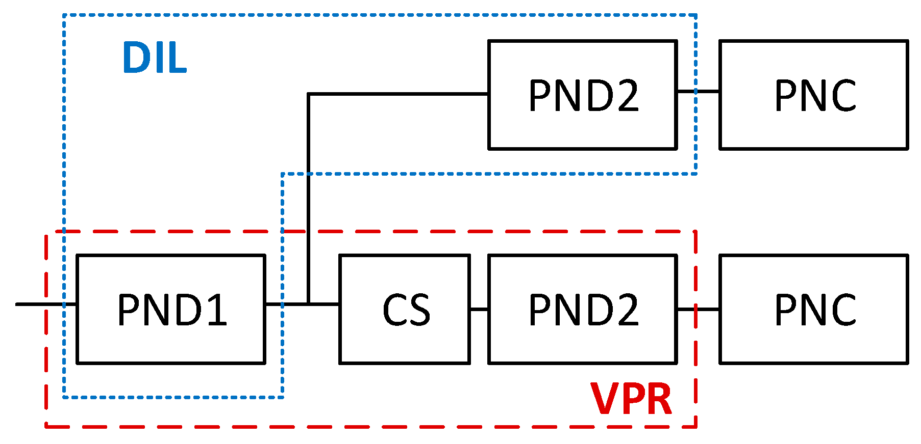
  • A Dilution system (DIL) for TPN10 or a volatile particle remover (VPR) for SPN10. The DIL dilutes the aerosol sample with clean air and the VPR dilutes the aerosol sample and removes volatile particles. For SPN10, the setup mandates a catalytic stripper at 350 °C to remove volatile particles. The minimum total dilution (before and/or after the catalytic stripper) must be at least 10:1.
  • Particle number counter (PNC) that counts particles from approximately 10 nm electrical mobility diameter and larger.
  • Internal tubing, abbreviated as internal transfer line (ITL), connects the DIL or VPR to the PNC.
The last three parts (DIL or VPR, ITL, and PNC) comprise the “PN system”. To ensure minimal particle losses, tubes upstream of the PN system may have only one bend complementing other technical requirements (e.g., maximum length, allowed ranges for internal diameters, and maximum residence time). The particle number setup (i.e., all parts from the nozzle to the PNC, including the splitter) must be of electrically conductive materials to avoid reactions with the brake particles. Using stainless steel with an electropolished finish (or equivalent) provides an ultra-clean and ultra-fine surface for the nozzle and the probe. The particle number setup must be electrically grounded to avoid electrical/electrostatic effects.
Figure 1 summarizes the allowed PN measurement configurations. The preferred setup uses two sampling probes for the PN emissions measurements, one for TPN10 and one for SPN10. The two-probe setup may come in two configurations:
  • With the cyclonic separator directly mounted to the probe’s outlet and followed by the PTT;
  • With the cyclonic separator directly mounted to the inlet of the DIL or VPR and preceded by the PTT.
Alternatively, a single sampling probe for TPN10 and SPN10 may apply an appropriate flow-splitting device using three possible configurations (for details see Appendix A, Figure A1):

2.2. Technical Specifications

Figure 2 gives a detailed overview of the technical requirements for the PN setup. Many available solutions in the market fulfill the UN GTR requirements, with some considerations below.
The probe’s diameter range (10–18 mm) and the residence time restriction of 3 s translates to a minimum flow rate of 1.6–5.1 L/min (Reynolds numbers 215–370), depending on the probe diameter. The setup can use higher flow rates without the risk of entering into a turbulent regime, which typically starts at Reynolds numbers > 2000–4000.
The choice of the nozzle for achieving isokinetic sampling depends on the tunnel flow rates and the probe and their respective inner diameters. Assuming a tunnel with an inner diameter of 200 mm (the acceptable range is 175–225 mm) and a flow rate as low as 200 m3/h (the minimum permitted operational flow must be between 100–300 m3/h), a minimum flow rate of 0.8 L/min in the probe would result in a 0.6 isokinetic ratio (the UN GTR allows 0.6–1.5). However, the residence time in a 10 mm probe would be 5.9 s which is almost double the maximum of 3 s allowed. Thus, the flow rate should be at least 1.6 L/min with the respective isokinetic ratio being 1.2. For the same tunnel settings, a 10 mm probe without any nozzle or a larger probe with a 10 mm nozzle and a 5 L/min probe flow rate would result in an isokinetic ratio of 0.6. On the other hand, a 10 times higher tunnel airflow (2000 m3/h) combined with a 4 mm nozzle would need at least 8 L/min probe airflow to exceed the minimum isokinetic ratio of 0.6. The application of an instrument with a 5 L/min air flow combined with a (moderately high) tunnel airflow of 1250 m3/h (with a 4 mm nozzle) or a low tunnel airflow of 200 m3/h and a 10 mm probe (or nozzle) yields the same isokinetic ratio of 0.6.

2.3. Background Levels

The PN concentration at the tunnel measured with the PN system must not exceed 20 #/cm3, which provides an upper limit for the background emissions (including the tunnel and brake enclosure). For flow rates between 100 m3/h and 2000 m3/h, the upper limit for the background emissions translate to 4.5 × 10⁷ to 9 × 10⁸ #/km, respectively.

3. Results

3.1. Scenarios

This section examines two scenarios:
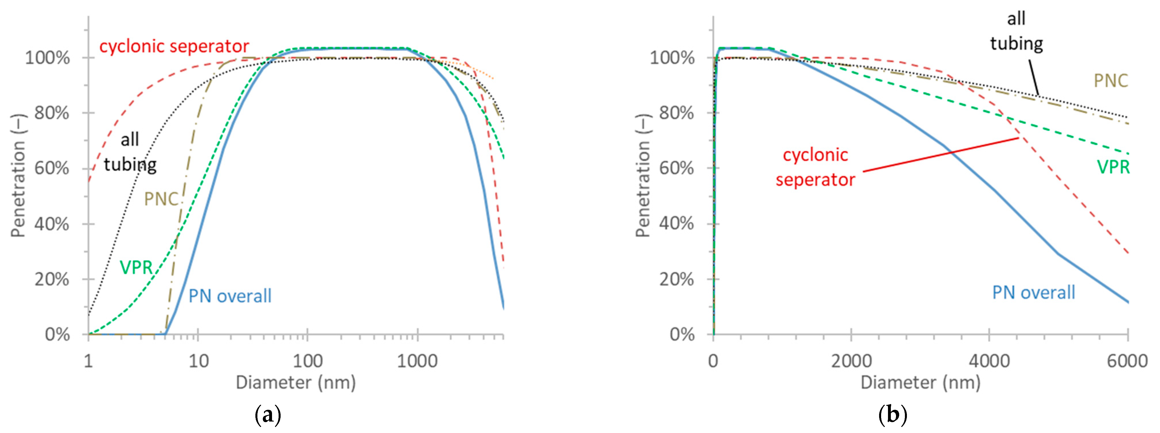
  • PN setup based on the specifications described above with minimum particle losses, and thus maximum penetration, abbreviated as “max penetration”.
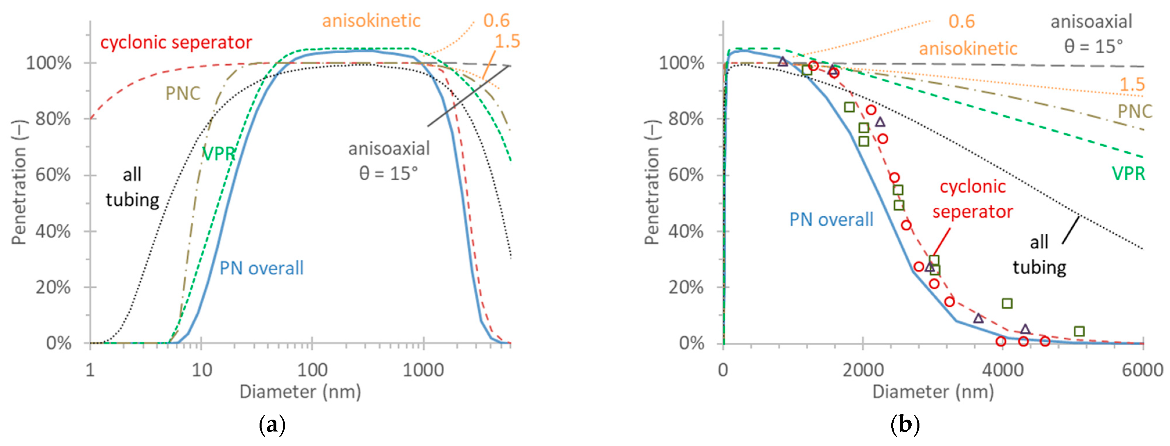
  • PN setup with all permissible flexibilities in the technical requirements maximizing particle losses, abbreviated as “min penetration”.
Table 1 summarizes the parameters for calculating the penetrations of the various parts of the “min penetration” and “max penetration” PN setups. The evaluations include cyclonic separators with two different upper cut-off sizes (2.5 μm and 5.0 μm).
The anisokinetic, anisoaxial, diffusional, inertial, and gravitational penetrations used the equations in the Ref. [49] based on [50,51,52]. Furthermore, the analysis assumes the electrostatic deposition to be negligible due to the required use of electrically conductive materials. The quantifications used the cyclonic separation of the pre-classifiers from the Ref. [49] based on the equations in the Ref. [53]. The theoretical curves of the cyclonic separators were also cross-checked with experimental penetrations from calibration certificates. No data were available for small nanoparticles (i.e., <10 nm) and some losses were expected. We assumed the losses of a tube with the same residence time and flow as in the cyclone. No losses were considered for the splitter (or that there is no splitter). This assumption is valid for equal flows at the two paths for sub-micron particles, as it is a regular check for the calibration of PNC instruments, with a split bias in the range of <1% (which is the experimental uncertainty). This assumption needs to be checked in the future for particles in the micrometer range. However, the technical requirements set a maximum difference for the flow and the particle losses between the two branches of 5%.
The VPR penetration is the ratio of the average particle concentration reduction factor (PCRF) to the PCRF at a specific size (see details in the Ref. [54]), given in the calibration certificates of the instruments. Note that this ratio can take values slightly higher than unity due to this definition in the regulation. There is no information available for losses at large sizes. The losses of different dilution concepts can give indications of expected losses of commercial systems. For example, ejector (venturi) diluters have negligible losses up to 1 μm [55,56], but they may become significant at bigger sizes depending on the design [57].
Similarly, orifice losses can be significant in the 1 μm range [58] or larger size ranges [59]. Rotating disks also have losses in the μm range [47]. The penetration of the PNC at small sizes was considered in the counting efficiency (CE) as given in the calibration certificates. At large sizes, such information is not available. For this reason, the published data from a 10 nm PNC were taken [48]. However, the penetration at large sizes is PNC model-dependent. For example, a 2.5 nm and a 23 nm PNC exhibited losses (or decreased counting efficiency) from 1 μm [60,61].
It should be noted that the diameters refer to aerodynamic diameters at large sizes and mobility diameters at small sizes. The “effective density” links the two diameters [62]. For this paper, this distinction is not essential and only the term “diameter” is used in the figures.

3.2. Penetration

Figure 3 presents the penetration of the “max penetration” PN setup with a 5.0 μm cyclonic separator (details in Table 1). Figure 3a focuses on the small particle sizes (5–1000 nm), while Figure 3b on the larger (1–6 μm). Note that the penetration can be slightly higher than unity due to how particle losses are considered in the VPR (or DIL). At small sizes, the VPR (or DIL) determines to a large degree the penetration curve and the contribution of diffusion, inertial, and gravitational losses in the tubes are small. The PNC counting efficiency determines for which particle size the overall penetration drops to zero. At large sizes, the cyclonic separator dictates the penetration curve, but the contribution of the VPR, PNC, and tubing is also essential. However, this does not occur at sizes smaller than 2.0–2.5 μm, which seems to be the most relevant for brake emissions measurements [29,38,41]. A cyclonic separator with a larger cut-off size does not significantly improve the penetrations even for this “max penetration” scenario. The 50% penetration with a 5 μm cyclonic separator is 4.2 μm, while with a 10 μm cyclonic separator is 5.0 μm. Thus, the risk of higher contamination of the PN systems is not accompanied by a significant improvement in penetration at large sizes.
Figure 4 presents the penetration of the “min penetration” PN setup using a 2.5 μm cyclonic separator (details in Table 1). Figure 4a focuses on the small particle sizes (5–1000 nm), while Figure 4b on the larger (1–6 μm). While diffusion, gravitational, and inertial losses in the tubes and the PNC counting efficiency are relevant, the VPR determines the penetration curve at small sizes. On the other hand, the cyclonic separator determines the penetration curve at large sizes. For this reason, anisokinetic or anisoaxial sampling is not considered necessary; however, it becomes crucial for particles larger than 2.5 μm.

4. Discussion

4.1. Penetration for Various Size Distributions

The particle loss analysis in the results section showed the PN measurements cover a range of approximately 10 nm to 10 μm. The particle size range with penetration above 50% is determined mainly by the VPR (or DIL) at the lower end and the cyclonic separator at the upper end. For most commercial PN systems with a 2.5 μm cyclonic separator, the penetration is above 50% between approximately 15 nm and 2 μm. Table 2 presents the penetration for different size distributions at the inlet of the PN setup. The GSDs for large particles were assumed to be two, based on fittings of published size distributions (e.g., [29]). Also, the calculations apply the parameters from Table 1 for 2.5 and 5 μm cyclonic separators. Lastly, Table 2 summarizes the results with the “max penetration” setup of Figure 3 and the “min penetration” setup of Figure 4. Although not shown, assuming a much larger GSD of 2.5 would result in <4% (absolute) differences for all sizes.
As expected, the overall penetration of the “min penetration” setup after the 2.5 μm cyclonic separator is around 50% when the inlet size distribution has a geometric mean diameter (GMD) of 15 nm or 2000 nm. The penetration of the setup is above 80% in the size range of 30 nm to 1000 nm, while achieving maximum penetration for size distributions with GMDs in the range of 50 nm to 700 nm.
Table 2 also lists the penetration using a 5 μm cyclonic separator for the “min penetration” setup. The 50% penetration is below 3 μm and not at the cyclonic separator’s 50% penetration (5 μm) because the losses in the other parts of the setup become dominant. Cyclonic separators with larger cut-off sizes do not provide any advantage in determining the particle number concentration due to the relatively high losses in this setup.
The other interesting finding is that a nucleation mode around 20 nm has a penetration of about 65% similar to the penetration of 1.5 μm solid particles. For this reason, the concentration ratio between the two modes of 20 nm and 1.5 μm does not significantly impact the results. The results differ when particles in the 50 nm to 700 nm range are measured. For example, when one peak is at 100 nm the penetration is at least 93% when the ratio of the two modes is 4:1 or higher. In these cases, the cut-off size of the cyclonic separator does not play a significant role because the smaller particles dominate the particle concentration.
The “max penetration” setup has 50% penetrations for GMDs closer to 10 nm and 2–3 μm. As a result, 20 nm and 1.5 μm size distributions demonstrate much higher penetrations of 75–80% compared to the 63–70% penetrations of the “min penetration” setup. When measuring 100 nm and 1.5 μm size distributions, differences between the two setups are minimal (85–100% vs. 83–98%). Thus, the importance of optimizing the setup and using a larger than 2.5 μm cyclonic separator depends on the expected size distributions.
The calculations only present the PN system’s penetration for the different scenarios. Losses also occur in the brake enclosure and the sampling tunnel; however, these are outside of the scope of this paper. Depending on the enclosure design and airflows in the tunnel, the penetration for 10 μm particles can range from 65–70% [29,63,64] to 90–95% [32,65]. One study using a heated line up to the instrument’s inlet estimated 31% sedimentation (gravitational) losses of 10 μm particles [66]. Another study found negligible losses for an onboard vehicle sampling system in the 40–700 nm range. Outside that range and depending on the flow rate of the sampling system, losses increased, reaching 40% to 80% for 10 μm particles [41]. Similar computational fluid dynamics (CFD) results for other onboard vehicle systems estimated approximately 90% penetration at 4–5 μm and 40% at 10 μm [67,68].
No data are available for penetrations of the complete PN setup because the technical specifications from the UN GTR are recent; thus, no such systems are available for evaluation. Previous studies evaluated instruments connected directly to the tunnel and, in many cases, with minimum lengths of tubes or no dilution or VPR units. One study [29] assessed the penetration from the brake enclosure to the measurement instrument and found it to be above 93% at 55–65 nm, with most of the losses attributed to coagulation. These results align with this research’s estimations (96% to 99%).

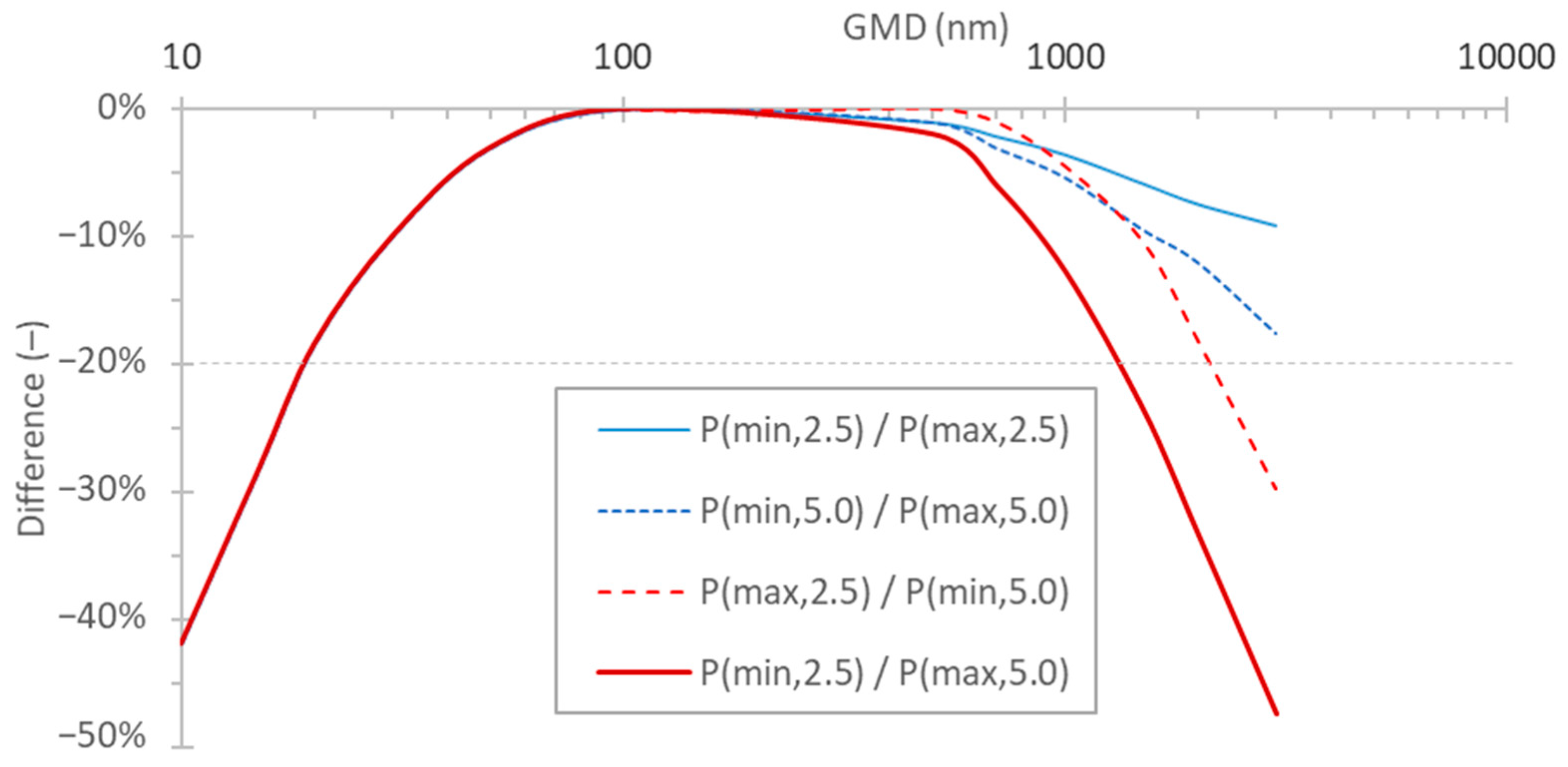
4.2. Differences between PN Setups

Two PN setups may exhibit differences due to the variations in penetration levels in the various parts or components. The results from Table 2 allow the engineer to estimate the maximum differences anticipated between various PN setups sampling from the same tunnel. Figure 5 provides an overview of the anticipated differences between various setups in Table 2 as a function of the measured geometric mean diameter (GMD). The differences were calculated based on the penetrations for various size distributions. For example, a setup with 60% penetration will measure 25% less than a setup with 80% penetration. For small particles, one curve is plotted, reflecting the difference between the “max penetration” and “min penetration” scenarios. Commercial systems are much closer; thus, smaller differences are expected [69].
Nevertheless, even for the opposite cases (“min penetration” and “max penetration” setups), the differences are less than 20% for GMDs of 20 nm or larger. The 20% value was chosen arbitrarily as an acceptable level of difference and the differences are negligible in the range of 50 nm to 500 nm. For large sizes, the blue lines are differences between the “min penetration” and “max penetration” setups using the same cut-off size cyclonic separators. In contrast, the red lines show the differences between the “min penetration” and “max penetration” setups using different cut-off sizes cyclonic separators. The most significant differences are for cyclonic separators with different cut-off sizes. When the setups have cyclonic separators with the same cut-off size, the differences are below 20%, even at 3 μm. System setup differences could be further reduced (or increase the size range with acceptable differences) by focusing on the cyclonic separator and the VPR for size distributions peaking at the setup’s smaller and higher cut-off sizes.
The penetration calculation presented so far are independent of the PN concentration. However, one mechanism not considered in penetration calculations is agglomeration or accumulation, which depends on the PN concentration. High particle concentrations in the tunnel promote agglomeration in the probe and transfer tube resulting in lower concentrations and larger particle sizes. Depending on residence time in the tubing up to the first dilution, agglomeration can be significant at concentrations above 107 #/cm3. For example, a 107 #/cm3 concentration for a 50 nm size distribution reduces by 1.5% with a 3 s residence time. At 108 #/cm3 the concentration reduces by 13%. In practice, such differences could be significant between setups with and without PTT (max residence time 1 s) and different flow rates that can result in differences in the residence time in the probe (max residence time 3 s). However, concentrations of 107 #/cm3 are rare in light-duty vehicles during everyday driving.
On the other hand, very low concentrations, close to the background levels (approximately 5 × 10⁸ #/km, see Section 2.3) mask any differences due to different penetrations and are due to the different background levels.

4.3. Significance of Upper Cut-Point

The number-to-mass ratio as a function of GMD puts the significance of the losses at the larger sizes in perspective. Table 3 presents the relationship between number and mass for various size distributions. For example, a size distribution of GMD = 200 nm possesses a ratio of 2.60 × 10¹⁰ #/mg. In other words, a limit of 1 mg/km (per brake) would be equivalent to 2.60 × 10¹⁰ #/km having a density of unity. The same limit would translate to less than 4.3 × 10⁸ #/km for particles 1000 nm or larger, which is the background level of the PN setup (see Section 2.3). Thus, the importance of particle numbers for large particle distributions is minor if there is a mass limit. Thus, the number concentration of large particles can be meaningful only if their mass emissions are very high.
Considering the Euro 7 brake PM mass proposal of 7 mg/km per vehicle, any PN limit above 1 × 10¹⁰ #/km can capture high PN emitters that still fulfil the PM limit (but with GMDs < 500 nm). Thus, the PM mass metric is very important to capture high emitters with large GMDs. It should be emphasized that the 1 × 10¹⁰ #/km value is 60 times lower than the exhaust PN limit of 6 × 10¹¹ #/km.

4.4. Comparison with Exhaust Setups

Table 4 summarizes the main differences between the exhaust and brakes PN setups.
The most important differences between the brake setups are:
  • Isokinetic sampling is required; however, with a relatively relaxed range of tolerance: 0.6–1.5.
  • A cyclonic separator is required in the brake setup but is only recommended for the exhaust PN systems.
  • The primary dilution of the brakes VPR does not need heating to 150 °C; however, the VPR needs a catalytic stripper at 350 °C. For exhaust systems, the first dilution must be hot (>150 °C), and the catalytic stripper is required only for the recommended system provided as an example in the exhaust regulation. The volatile removal efficiency requirements with tetracontane particles are identical (see Figure 2).
  • The primary dilution factor of the brakes system is undefined as long as the total dilution is at least 10:1, while for the exhaust PN systems, the primary dilution has to be at least 10:1.
PN systems in the market for exhaust emissions measurements already fulfill the brake emissions requirements of the VPR, ITL, and PNC for measuring SPN10. Turning off all their heaters will fulfill the requirements for DIL, ITL, and PNC for the measurement of TPN10, where the only requirement is that the diluted sample temperature is <38 °C. This requirement is based on the typical saturator temperature of the PNCs at that range. There is no exhaust regulation for TPN10 but only recommendations [45].
There are two critical differences compared to the exhaust measurement systems, which provide flexibility for future solutions related to the primary dilution:
  • It does not have a minimum ratio as long as the total dilution is 10:1 or higher.
  • It does not need to be hot.
This flexibility allows a combined solution for the measurements of solid and total PN within one system (Figure 6). However, the current UN GTR does not allow such a solution for regulatory measurements; thus, such solutions are suitable only for research projects or onboard vehicle systems. There is a current proposal for exhaust PN systems for measurement of TPN measurements which are not regulated [45].

5. Conclusions

In this paper, we described the PN setup of the current draft brake’s GTR. The losses in the parts (nozzle, probe, tubing, cyclone, diluter, and particle counter) were estimated for a “max penetration” case and a “min penetration” case using all the flexibilities allowed. Depending on the case, the penetration of the setup was 50% for size distributions with means 10–15 nm and 2000–3000 nm, while >95% was in the range of 50 nm to 700 nm. Based on the two extreme cases, in the field, differences of less than 20% for GMDs of 20 nm or larger are expected due to losses in the setup. Theoretical estimations showed that in the case of a mass limit, a PN limit makes sense to capture small particles that do not contribute to the mass. One to two orders of magnitude higher than the background level’s PN limit can capture particles < 500 nm that fulfill the PM’s proposed limit of 7 mg/km. The solid PN setup was based on the exhaust PN setup with some small differences.

Author Contributions

Conceptualization, T.G. and B.G.; formal analysis, B.G.; writing—original draft preparation, T.G. and B.G.; writing—review and editing, all. All authors have read and agreed to the published version of the manuscript.

Funding

This research received no external funding.

Institutional Review Board Statement

Not applicable.

Informed Consent Statement

Not applicable.

Data Availability Statement

Not applicable.

Conflicts of Interest

The authors declare no conflict of interest.

Disclaimer

The opinions expressed in this manuscript are those of the authors and should in no way be considered to represent an official opinion of the European Commission, and/or the instrument manufacturers. Mention of trade names or commercial products does not constitute endorsement or recommendation by the European Commission, the instrument manufacturers, and/or the authors.

Appendix A

In the case of a single sampling probe for TPN10 and SPN10 there are three possible configurations using a splitter (Figure A1):
Figure A1. Particle number (PN) setup parts and layouts using one-probe. PN system in red (three last parts). The asterisk (*) indicates a one-probe configuration not allowed in the current GTR version. Cycl. = cyclonic separator; DIL = diluter; ITL = internal transfer line; PNC = particle number counter; PTT = particle transfer tube; Split. = flow-splitting device; VPR = volatile particle remover.
Atmosphere 14 00103 g0a1
  • With the cyclonic separator directly mounted to the probe’s outlet and followed by the flow-splitting device and the PTT;
  • With the cyclonic separator directly mounted to the inlet of the PN system and preceded by the flow-splitting device and the PTT, respectively;
  • With the cyclonic separator directly mounted to the inlet of the PN system and preceded by the PTT and the flow-splitting device, respectively.
Note that the current version of the GTR does not allow the single-probe configuration with the order: splitter, cyclonic separator, and PTT and combinations (e.g., TPN10 with PTT and cyclonic separator after the splitter, while SPN10 with cyclonic separator and PTT after the splitter).

References

  1. Health Effects Institute. State of Global Air 2020; Health Effects Institute: Boston, MA, USA, 2020. [Google Scholar]
  2. Hamanaka, R.B.; Mutlu, G.M. Particulate Matter Air Pollution: Effects on the Cardiovascular System. Front. Endocrinol. 2018, 9, 680. [Google Scholar] [CrossRef] [Green Version]
  3. Zhang, R.; Wang, G.; Guo, S.; Zamora, M.L.; Ying, Q.; Lin, Y.; Wang, W.; Hu, M.; Wang, Y. Formation of Urban Fine Particulate Matter. Chem. Rev. 2015, 115, 3803–3855. [Google Scholar] [CrossRef]
  4. European Environmental Agency (EEA). Air Quality in Europe 2022. 2022. Available online: https://www.eea.europa.eu/publications/air-quality-in-europe-2022 (accessed on 1 December 2022).
  5. Karagulian, F.; Belis, C.A.; Dora, C.F.C.; Prüss-Ustün, A.M.; Bonjour, S.; Adair-Rohani, H.; Amann, M. Contributions to Cities’ Ambient Particulate Matter (PM): A Systematic Review of Local Source Contributions at Global Level. Atmos. Environ. 2015, 120, 475–483. [Google Scholar] [CrossRef]
  6. Habre, R.; Girguis, M.; Urman, R.; Fruin, S.; Lurmann, F.; Shafer, M.; Gorski, P.; Franklin, M.; McConnell, R.; Avol, E.; et al. Contribution of Tailpipe and Non-Tailpipe Traffic Sources to Quasi-Ultrafine, Fine and Coarse Particulate Matter in Southern California. J. Air Waste Manag. Assoc. 2021, 71, 209–230. [Google Scholar] [CrossRef] [PubMed]
  7. Trombetti, M.; Thunis, P.; Bessagnet, B.; Clappier, A.; Couvidat, F.; Guevara, M.; Kuenen, J.; López-Aparicio, S. Spatial Inter-Comparison of Top-down Emission Inventories in European Urban Areas. Atmos. Environ. 2018, 173, 142–156. [Google Scholar] [CrossRef]
  8. Fujitani, Y.; Takahashi, K.; Saitoh, K.; Fushimi, A.; Hasegawa, S.; Kondo, Y.; Tanabe, K.; Takami, A.; Kobayashi, S. Contribution of Industrial and Traffic Emissions to Ultrafine, Fine, Coarse Particles in the Vicinity of Industrial Areas in Japan. Environ. Adv. 2021, 5, 100101. [Google Scholar] [CrossRef]
  9. Weber, S.; Salameh, D.; Albinet, A.; Alleman, L.Y.; Waked, A.; Besombes, J.-L.; Jacob, V.; Guillaud, G.; Meshbah, B.; Rocq, B.; et al. Comparison of PM10 Sources Profiles at 15 French Sites Using a Harmonized Constrained Positive Matrix Factorization Approach. Atmosphere 2019, 10, 310. [Google Scholar] [CrossRef] [Green Version]
  10. Seibert, R.; Nikolova, I.; Volná, V.; Krejčí, B.; Hladký, D. Air Pollution Sources’ Contribution to PM2.5 Concentration in the Northeastern Part of the Czech Republic. Atmosphere 2020, 11, 522. [Google Scholar] [CrossRef]
  11. Kosmopoulos, G.; Salamalikis, V.; Matrali, A.; Pandis, S.N.; Kazantzidis, A. Insights about the Sources of PM2.5 in an Urban Area from Measurements of a Low-Cost Sensor Network. Atmosphere 2022, 13, 440. [Google Scholar] [CrossRef]
  12. Firląg, S.; Rogulski, M.; Badyda, A. The Influence of Marine Traffic on Particulate Matter (PM) Levels in the Region of Danish Straits, North and Baltic Seas. Sustainability 2018, 10, 4231. [Google Scholar] [CrossRef]
  13. Durán-Grados, V.; Rodríguez-Moreno, R.; Calderay-Cayetano, F.; Amado-Sánchez, Y.; Pájaro-Velázquez, E.; Nunes, R.A.O.; Alvim-Ferraz, M.C.M.; Sousa, S.I.V.; Moreno-Gutiérrez, J. The Influence of Emissions from Maritime Transport on Air Quality in the Strait of Gibraltar (Spain). Sustainability 2022, 14, 12507. [Google Scholar] [CrossRef]
  14. Yusuf, A.A.; Inambao, F.L.; Ampah, J.D. Evaluation of Biodiesel on Speciated PM2.5, Organic Compound, Ultrafine Particle and Gaseous Emissions from a Low-Speed EPA Tier II Marine Diesel Engine Coupled with DPF, DEP and SCR Filter at Various Loads. Energy 2022, 239, 121837. [Google Scholar] [CrossRef]
  15. Diesel Net. Emission Standards. 2022. Available online: https://dieselnet.com/standards/ (accessed on 1 December 2022).
  16. Giechaskiel, B.; Maricq, M.; Ntziachristos, L.; Dardiotis, C.; Wang, X.; Axmann, H.; Bergmann, A.; Schindler, W. Review of Motor Vehicle Particulate Emissions Sampling and Measurement: From Smoke and Filter Mass to Particle Number. J. Aerosol Sci. 2014, 67, 48–86. [Google Scholar] [CrossRef]
  17. Giechaskiel, B.; Melas, A.; Martini, G.; Dilara, P. Overview of Vehicle Exhaust Particle Number Regulations. Processes 2021, 9, 2216. [Google Scholar] [CrossRef]
  18. European Environment Agency. Air Quality in Europe: 2020 Report; Publications Office of the European Union: Luxembourg, 2020; ISBN 978-92-9480-29.
  19. Harrison, R.M.; Allan, J.; Carruthers, D.; Heal, M.R.; Lewis, A.C.; Marner, B.; Murrells, T.; Williams, A. Non-Exhaust Vehicle Emissions of Particulate Matter and VOC from Road Traffic: A Review. Atmos. Environ. 2021, 262, 118592. [Google Scholar] [CrossRef]
  20. Grange, S.K.; Fischer, A.; Zellweger, C.; Alastuey, A.; Querol, X.; Jaffrezo, J.-L.; Weber, S.; Uzu, G.; Hueglin, C. Switzerland’s PM10 and PM2.5 Environmental Increments Show the Importance of Non-Exhaust Emissions. Atmos. Environ. X 2021, 12, 100145. [Google Scholar] [CrossRef]
  21. Piscitello, A.; Bianco, C.; Casasso, A.; Sethi, R. Non-Exhaust Traffic Emissions: Sources, Characterization, and Mitigation Measures. Sci. Total Environ. 2021, 766, 144440. [Google Scholar] [CrossRef]
  22. Woo, S.-H.; Jang, H.; Lee, S.-B.; Lee, S. Comparison of Total PM Emissions Emitted from Electric and Internal Combustion Engine Vehicles: An Experimental Analysis. Sci. Total Environ. 2022, 842, 156961. [Google Scholar] [CrossRef]
  23. Hagino, H.; Oyama, M.; Sasaki, S. Airborne Brake Wear Particle Emission Due to Braking and Accelerating. Wear 2015, 334–335, 44–48. [Google Scholar] [CrossRef]
  24. Grigoratos, T.; Martini, G. Brake Wear Particle Emissions: A Review. Environ. Sci. Pollut. Res. 2015, 22, 2491–2504. [Google Scholar] [CrossRef]
  25. Mathissen, M.; Grigoratos, T.; Lahde, T.; Vogt, R. Brake Wear Particle Emissions of a Passenger Car Measured on a Chassis Dynamometer. Atmosphere 2019, 10, 556. [Google Scholar] [CrossRef] [Green Version]
  26. Mellios, G.; Ntziachristos, L. Evaporation and Brake Wear Control. Onine AGVES Meeting. 8 April 2021. Available online: https://circabc.europa.eu/sd/a/1c0efc15-8507-4797-9647-97c12d82fa28/agves-2021-04-08-evap_non-exh.pdf (accessed on 1 December 2022).
  27. European Commission. Directorate General for Internal Market, Industry, Entrepreneurship and SMEs. In Technical Studies for the Development of Euro 7: Testing, Pollutants and Emission Limits; Publications Office of the European Union: Luxembourg, 2022; ISBN 978-92-76-56545-1. [Google Scholar]
  28. Grigoratos, T.; Mathissen, M.; Gramstat, S.; Mamakos, A.; Vedula, R.; Agudelo, C.; Grochowicz, J.; Giechaskiel, B. Interlaboratory Study on Brake Particle Emissions–Part I: Particulate Matter Mass Emissions. Atmosphere 2023. under review. [Google Scholar]
  29. Mamakos, A.; Arndt, M.; Hesse, D.; Augsburg, K. Physical Characterization of Brake-Wear Particles in a PM10 Dilution Tunnel. Atmosphere 2019, 10, 639. [Google Scholar] [CrossRef] [Green Version]
  30. Mamakos, A.; Kolbeck, K.; Arndt, M.; Schröder, T.; Bernhard, M. Particle Emissions and Disc Temperature Profiles from a Commercial Brake System Tested on a Dynamometer under Real-World Cycles. Atmosphere 2021, 12, 377. [Google Scholar] [CrossRef]
  31. Farwick zum Hagen, F.H.; Mathissen, M.; Grabiec, T.; Hennicke, T.; Rettig, M.; Grochowicz, J.; Vogt, R.; Benter, T. On-Road Vehicle Measurements of Brake Wear Particle Emissions. Atmos. Environ. 2019, 217, 116943. [Google Scholar] [CrossRef]
  32. zum Hagen, F.H.F.; Mathissen, M.; Grabiec, T.; Hennicke, T.; Rettig, M.; Grochowicz, J.; Vogt, R.; Benter, T. Study of Brake Wear Particle Emissions: Impact of Braking and Cruising Conditions. Environ. Sci. Technol. 2019, 53, 5143–5150. [Google Scholar] [CrossRef]
  33. Mathissen, M.; Grigoratos, T.; Gramstat, S.; Mamakos, A.; Vedula, R.; Agudelo, C.; Grochowicz, J.; Giechaskiel, B. Interlaboratory Study on Brake Particle Emissions–Part II: Particle Number Emissions. Atmosphere 2023. under review. [Google Scholar]
  34. Alemani, M.; Nosko, O.; Metinoz, I.; Olofsson, U. A Study on Emission of Airborne Wear Particles from Car Brake Friction Pairs. SAE Int. J. Mater. Manf. 2015, 9, 147–157. [Google Scholar] [CrossRef]
  35. Kukutschová, J.; Moravec, P.; Tomášek, V.; Matějka, V.; Smolík, J.; Schwarz, J.; Seidlerová, J.; Šafářová, K.; Filip, P. On Airborne Nano/Micro-Sized Wear Particles Released from Low-Metallic Automotive Brakes. Environ. Pollut. 2011, 159, 998–1006. [Google Scholar] [CrossRef] [PubMed]
  36. Nosko, O.; Olofsson, U. Effective Density of Airborne Wear Particles from Car Brake Materials. J. Aerosol Sci. 2017, 107, 94–106. [Google Scholar] [CrossRef]
  37. Agudelo, C.; Vedula, R.T.; Collier, S.; Stanard, A. Brake Particulate Matter Emissions Measurements for Six Light-Duty Vehicles Using Inertia Dynamometer Testing; SAE 2020-01–1637; SAE International: Warrendale, PA, USA, 2020. [Google Scholar]
  38. Stanard, A.; DeFries, T.; Palacios, C.; Kishan, S. Brake and Tire Wear Emissions; ERG: Concord, MA, USA, 2021. [Google Scholar]
  39. Hagino, H.; Oyama, M.; Sasaki, S. Laboratory Testing of Airborne Brake Wear Particle Emissions Using a Dynamometer System under Urban City Driving Cycles. Atmos. Environ. 2016, 131, 269–278. [Google Scholar] [CrossRef] [Green Version]
  40. Kukutschová, J.; Filip, P. Review of Brake Wear Emissions. In Non-Exhaust Emissions; Elsevier: Amsterdam, The Netherlands, 2018; pp. 123–146. ISBN 978-0-12-811770-5. [Google Scholar]
  41. Andersson, J.; Campbell, M.; Marshall, I.; Kramer, L.; Norris, J. Measurement of Emissions from Brake and Tyre Wear. Final Report—Phase 1; T0018-TETI0037, Ricardo Ref. ED14775; Ricardo: London, UK, 2022. [Google Scholar]
  42. Fussell, J.C.; Franklin, M.; Green, D.C.; Gustafsson, M.; Harrison, R.M.; Hicks, W.; Kelly, F.J.; Kishta, F.; Miller, M.R.; Mudway, I.S.; et al. A Review of Road Traffic-Derived Non-Exhaust Particles: Emissions, Physicochemical Characteristics, Health Risks, and Mitigation Measures. Environ. Sci. Technol. 2022, 56, 6813–6835. [Google Scholar] [CrossRef]
  43. Grigoratos, T.; Agudelo, C.; Grochowicz, J.; Gramstat, S.; Robere, M.; Perricone, G.; Sin, A.; Paulus, A.; Zessinger, M.; Hortet, A.; et al. Statistical Assessment and Temperature Study from the Interlaboratory Application of the WLTP–Brake Cycle. Atmosphere 2020, 11, 1309. [Google Scholar] [CrossRef]
  44. Grigoratos, T.; Giechaskiel, B. Draft GTR—Proposed Way Forward. PMP Webex. 25 May 2022. Available online: https://wiki.unece.org/display/trans/pmp+web+conference+25.05.2022 (accessed on 1 December 2022).
  45. Giechaskiel, B.; Melas, A.; Martini, G.; Dilara, P.; Ntziachristos, L. Revisiting Total Particle Number Measurements for Vehicle Exhaust Regulations. Atmosphere 2022, 13, 155. [Google Scholar] [CrossRef]
  46. Mathissen, M.; Grochowicz, J.; Schmidt, C.; Vogt, R.; Farwick zum Hagen, F.H.; Grabiec, T.; Steven, H.; Grigoratos, T. A Novel Real-World Braking Cycle for Studying Brake Wear Particle Emissions. Wear 2018, 414–415, 219–226. [Google Scholar] [CrossRef]
  47. Zhang, S.; Liu, S.; Chen, Q. Particle Capture by a Rotating Disk in a Kitchen Exhaust Hood. Aerosol Sci. Technol. 2020, 54, 929–940. [Google Scholar] [CrossRef]
  48. Yli-Ojanperä, J.; Sakurai, H.; Iida, K.; Mäkelä, J.M.; Ehara, K.; Keskinen, J. Comparison of Three Particle Number Concentration Calibration Standards through Calibration of a Single CPC in a Wide Particle Size Range. Aerosol Sci. Technol. 2012, 46, 1163–1173. [Google Scholar] [CrossRef] [Green Version]
  49. Giechaskiel, B.; Arndt, M.; Schindler, W.; Bergmann, A.; Silvis, W.; Drossinos, Y. Sampling of Non-Volatile Vehicle Exhaust Particles: A Simplified Guide. SAE Int. J. Engines 2012, 5, 379–399. [Google Scholar] [CrossRef]
  50. Hinds, W.C. Aerosol Technology: Properties, Behavior, and Measurement of Airborne Particles, 2nd ed.; Wiley: New York, NY, USA, 1999; ISBN 978-0-471-19410-1. [Google Scholar]
  51. Baron, P.A.; Kulkarni, P.; Willeke, K. (Eds.) Aerosol Measurement: Principles, Techniques, and Applications, 3rd ed.; Wiley: Hoboken, NJ, USA, 2011; ISBN 978-0-470-38741-2. [Google Scholar]
  52. Vincent, J.H. Aerosol Sampling: Science, Standards, Instrumentation and Applications; John Wiley & Sons: Chichester, UK; Hoboken, NJ, USA, 2007; ISBN 978-0-470-02725-7. [Google Scholar]
  53. Dirgo, J.; Leith, D. Cyclone Collection Efficiency: Comparison of Experimental Results with Theoretical Predictions. Aerosol Sci. Technol. 1985, 4, 401–415. [Google Scholar] [CrossRef] [Green Version]
  54. Giechaskiel, B.; Melas, A. Impact of Material on Response and Calibration of Particle Number Systems. Atmosphere 2022, 13, 1770. [Google Scholar] [CrossRef]
  55. Helsper, C.; Mölter, W.; Haller, P. Representative Dilution of Aerosols by a Factor of 10,000. J. Aerosol Sci. 1990, 21, S637–S640. [Google Scholar] [CrossRef]
  56. Giechaskiel, B.; Ntziachristos, L.; Samaras, Z. Effect of Ejector Dilutors on Measurements of Automotive Exhaust Gas Aerosol Size Distributions. Meas. Sci. Technol. 2009, 20, 045703. [Google Scholar] [CrossRef]
  57. Shin, D.; Woo, C.G.; Hong, K.-J.; Kim, H.-J.; Kim, Y.-J.; Lee, G.-Y.; Chun, S.-N.; Hwang, J.; Han, B. Development of a New Dilution System for Continuous Measurement of Particle Concentration in the Exhaust from a Coal-Fired Power Plant. Fuel 2019, 257, 116045. [Google Scholar] [CrossRef]
  58. Liu, P.S.K.; Deng, R.; Smith, K.A.; Williams, L.R.; Jayne, J.T.; Canagaratna, M.R.; Moore, K.; Onasch, T.B.; Worsnop, D.R.; Deshler, T. Transmission Efficiency of an Aerodynamic Focusing Lens System: Comparison of Model Calculations and Laboratory Measurements for the Aerodyne Aerosol Mass Spectrometer. Aerosol Sci. Technol. 2007, 41, 721–733. [Google Scholar] [CrossRef]
  59. Hwang, T.-H.; Kim, S.-H.; Kim, S.H.; Lee, D. Reducing Particle Loss in a Critical Orifice and an Aerodynamic Lens for Focusing Aerosol Particles in a Wide Size Range of 30 Nm–10 Μm. J. Mech. Sci. Technol. 2015, 29, 317–323. [Google Scholar] [CrossRef]
  60. Sang-Nourpour, N.; Olfert, J.S. Calibration of Optical Particle Counters with an Aerodynamic Aerosol Classifier. J. Aerosol Sci. 2019, 138, 105452. [Google Scholar] [CrossRef]
  61. Tran, S.; Iida, K.; Yashiro, K.; Murashima, Y.; Sakurai, H.; Olfert, J.S. Determining the Cutoff Diameter and Counting Efficiency of Optical Particle Counters with an Aerodynamic Aerosol Classifier and an Inkjet Aerosol Generator. Aerosol Sci. Technol. 2020, 54, 1335–1344. [Google Scholar] [CrossRef]
  62. Kelly, W.P.; McMurry, P.H. Measurement of Particle Density by Inertial Classification of Differential Mobility Analyzer–Generated Monodisperse Aerosols. Aerosol Sci. Technol. 1992, 17, 199–212. [Google Scholar] [CrossRef]
  63. Sanders, P.G.; Xu, N.; Dalka, T.M.; Maricq, M.M. Airborne Brake Wear Debris: Size Distributions, Composition, and a Comparison of Dynamometer and Vehicle Tests. Environ. Sci. Technol. 2003, 37, 4060–4069. [Google Scholar] [CrossRef]
  64. Mamakos, A.; Arndt, M.; Hesse, D.; Hamatschek, C.; Augsburg, K. Comparison of Particulate Matter and Number Emissions from a Floating and a Fixed Caliper Brake System of the Same Lining Formulation; SAE 2020-01-1633; SAE International: Warrendale, PA, USA, 2020. [Google Scholar]
  65. Perricone, G.; Wahlström, J.; Olofsson, U. Towards a Test Stand for Standardized Measurements of the Brake Emissions. Proc. Inst. Mech. Eng. Part J. Automob. Eng. 2016, 230, 1521–1528. [Google Scholar] [CrossRef]
  66. Perricone, G.; Matĕjka, V.; Alemani, M.; Wahlström, J.; Olofsson, U. A Test Stand Study on the Volatile Emissions of a Passenger Car Brake Assembly. Atmosphere 2019, 10, 263. [Google Scholar] [CrossRef] [Green Version]
  67. Hesse, D.; Augsburg, K. Real Driving Emissions Measurement of Brake Dust Particles; SAE 2019-01-2138; SAE International: Warrendale, PA, USA, 2019. [Google Scholar]
  68. Feißel, T.; Hesse, D.; Augsburg, K.; Gramstat, S. Measurement of Vehicle Related Non Exhaust Particle Emissions under Real Driving Conditions. In Proceedings of the Euro Brake 2020, Online, 16 June 2020. [Google Scholar]
  69. Giechaskiel, B.; Lähde, T.; Melas, A.D.; Valverde, V.; Clairotte, M. Uncertainty of Laboratory and Portable Solid Particle Number Systems for Regulatory Measurements of Vehicle Emissions. Environ. Res. 2021, 197, 111068. [Google Scholar] [CrossRef]
Figure 1. Particle number (PN) setup parts and layouts with two-probe. PN system in red (three last red boxes). The one-probe layout can be found in the Appendix A. Cycl. = cyclonic separator; DIL = diluter; ITL = internal transfer line; PNC = particle number counter; PTT = particle transfer tube; Split. = flow-splitting device; VPR = volatile particle remover.
Atmosphere 14 00103 g001
Figure 2. Overview of the technical requirements of the particle number (PN) setup. acc = accuracy; CE = counting efficiency; d = diameter; dev = deviation; DF = dilution factor; DIL = diluter; HEPA = high-efficiency particle air filter; L = length; noz = nozzle; P = penetration; p = pressure; PAO = polyalphaolefin; PCRF = particle concentration reduction factor; PNC = particle number counter; PND = particle number diluter; Q = flow; tun = tunnel; R = radius; RT = residence time; sp = splitter; V = velocity; VRE = volatile removal efficiency; VPR = volatile particle remover.
Atmosphere 14 00103 g002
Figure 3. Penetration of the PN setup assuming minimum losses and using a 5 μm cyclonic separator (“max penetration” setup): (a) logarithmic x-axis; (b) linear x-axis.
Atmosphere 14 00103 g003
Figure 4. Penetration of the PN setup assuming maximum flexibilities from the technical requirements and using a 2.5 μm cyclonic separator (“min penetration” setup): (a) logarithmic x-axis; (b) linear x-axis. Symbols (squares, triangles, circles) are experimental penetrations from three cyclonic separators.
Atmosphere 14 00103 g004
Figure 5. Differences between various setups with max penetration (“max”) and min penetration (“min”) setups and cyclonic separators of 2.5 μm and 5.0 μm.
Atmosphere 14 00103 g005
Figure 6. PN system combining total and solid particle number measurements. CS = catalytic stripper; DIL = diluter; PNC = particle number counter; PND = particle number diluter; VPR = volatile particle remover.
Atmosphere 14 00103 g006
Table 1. Assumed parameters for the estimation of particle losses for the two scenarios.
Part 1“Max Penetration” Setup“Min Penetration” Setup
NozzleIsoaxial θ = 0°Anisoaxial θ = 15°
NozzleIsokinetic ratio = 1.0Anisokinetic ratio = 1.5
ProbeQpro = 5 L/min, dpro = 10 mm, Lpro = 1 mQpro = 5 L/min, dpro = 10 mm, Lpro = 1 m
Splitternonenone
Probe bendNo bendRbend,pro = 40 mm
Transfer (PTT)No transfer tubeQPTT = 5 L/min, dPTT = 4 mm, LPTT = 5 m
PTT bendNo bendRbend,PTT = 100 mm
Internal (ITL)QITL = 1 L/min, dITL = 4 mm, LITL = 0.4 mQITL = 1 L/min, dITL = 4 mm, LITL = 1 m
ITL bendNo bendRbend,ITL = 40 mm
GravitationalOnly in the probe, ITLOnly in the probe, PTT, ITL
VPRP10nm = 52%, P15nm = 68%, P10nm = 30%, P15nm = 53%,
VPRP30nm = 92%, P50nm = 101%, P100nm = 104%P30nm = 87%, P50nm = 101%, P100nm = 105%
VPR50% at 8 μm [47]
PNCP10nm = 80%, P15nm = 95%, 50% at 9 μm [48]
1 Examining cyclonic separators at 2.5 μm and 5 μm (i.e., 50% penetration at 2.5 μm and 5.0 μm respectively).
Table 2. Calculated penetrations of two PN setups (with “min penetration” and “max penetration”) using 2.5 μm and 5.0 μm cyclonic separators. See Table 1 for details on the different setups.
Scenario“Min Penetration” Setup“Max Penetration” Setup
GMD1 (GSD1) and GMD2 (GSD2) with C1:C22.5 μm5.0 μm2.5 μm5.0 μm
10 nm (1.5) 25%25%43%43%
15 nm (1.5)46%46%64%64%
20 nm (1.5)62%62%76%76%
30 nm (1.5)81%81%90%90%
50 nm (1.5)96%96%99%99%
100 nm (2.0)101%101%101%101%
500 nm (2.0)99%100%100%101%
700 nm (2.0)93%96%95%99%
1000 nm (2.0)82%89%85%94%
1500 nm (2.0)65%77%69%85%
2000 nm (2.0)50%66%54%75%
3000 nm (2.0)30%47%33%57%
20 nm (1.5) and 1500 nm (2.0) with a ratio of 9:163%64%76%77%
20 nm (1.5) and 1500 nm (2.0) with a ratio of 4:163%65%75%78%
20 nm (1.5) and 1500 nm (2.0) with a ratio of 1:164%70%73%81%
100 nm (1.5) and 1500 nm (2.0) with a ratio of 9:197%98%98%100%
100 nm (1.5) and 1500 nm (2.0) with a ratio of 4:193%96%95%98%
100 nm (1.5) and 1500 nm (2.0) with a ratio of 1:183%89%85%93%
C = concentration; GMD = geometric mean diameter; GSD = geometric standard deviation.
Table 3. Relationship between number and mass for various size distributions, assuming a density of unity and a setup with a cut-off at 10 μm.
GMD
(nm)
GSD
(nm)
Number-to-Mass Ratio
(#/mg)
201.51.08 × 1014
601.72.36 × 1012
2002.02.60 × 1010
5002.01.69 × 109
10002.02.35 × 108
20002.00.45 × 108
30002.00.22 × 108
Table 4. Comparison of SPN10 system requirements for vehicle brake and exhaust emissions. The table lists only the standard requirements for the brake and exhaust systems; the additional requirements for the brake systems are in Figure 2.
PartSymbolBrakes (Non-Exhaust)Engine (Exhaust)
Nozzle-RequiredNot prescribed
Probe-RequiredNo requirements
(Typically a bend in the tunnel)
Pre-classifier-Cyclonic separatorRecommended
(Cyclone, Impactor, Hat)
d50%2.5–10 μm2.5–10 μm
P>80% (number) (d1.5μm)>99% (mass) (d1μm)
Transfer tubeFlowLaminarLaminar (Re < 1700)
RT<1 s<3 s
VPR-RequiredRequired
PND1RequiredRequired
DF≥10:1 (total)≥ 10:1 (Primary)
Tmix≥150 °C (recommended)≥150 °C (Required)
CSRequiredRequired
(at recommended system)
TCS350 °C (±10 °C)350 °C (±10 °C)
(at recommended system)
Internal tubingd≥4 mm≥4 mm
RT<1.0 s≤0.8 s
PNC-RequiredRequired
MaterialPAO, soot, silverPAO, soot
CS = catalytic stripper; d50% = diameter with 50% penetration; DF =dilution factor; P = penetration; PAO = polyalphaolefin; PNC = particle number counter; PND = particle number diluter; RT = residence time; T = temperature; VPR = volatile particle remover.
Disclaimer/Publisher’s Note: The statements, opinions and data contained in all publications are solely those of the individual author(s) and contributor(s) and not of MDPI and/or the editor(s). MDPI and/or the editor(s) disclaim responsibility for any injury to people or property resulting from any ideas, methods, instructions or products referred to in the content.

