
Prediction of PM2.5 Concentration in Ningxia Hui Autonomous Region Based on PCA-Attention-LSTM
School of Mathematics and Information Science, North Minzu University, Yinchuan 750021, China
*
Author to whom correspondence should be addressed.
Atmosphere 2022, 13(9), 1444; https://doi.org/10.3390/atmos13091444
Submission received: 30 July 2022
/
Revised: 25 August 2022
/
Accepted: 26 August 2022
/
Published: 8 September 2022
(This article belongs to the Special Issue Air Pollution in China (2nd Edition))
Abstract
:The problem of air pollution has attracted more and more attention. PM2.5 is a key factor affecting air quality. In order to improve the prediction accuracy of PM2.5 concentration and make people effectively control the generation and propagation of atmospheric pollutants, in this paper, a long short-term memory neural network (LSTM) model based on principal component analysis (PCA) and attention mechanism (attention) is constructed, which first uses PCA to reduce the dimension of data, eliminate the correlation effect between indicators, and reduce model complexity, and then uses the extracted principal components to establish a PCA-attention-LSTM model. Simulation experiments were conducted on the air pollutant data, meteorological element data, and working day data of five cities in Ningxia from 2018 to 2020 to predict the PM2.5 concentration. The PCA-attention-LSTM model is compared with the support vector regression model (SVR), AdaBoost model, random forest model (RF), BP neural network model (BPNN), and long short-term memory neural network (LSTM). The results show that the PCA-attention-LSTM model is optimal; the correlation coefficients of the PCA-attention-LSTM model in Wuzhong, Yinchuan, Zhongwei, Shizuishan, and Guyuan are 0.91, 0.93, 0.91, 0.91, and 0.90, respectively, and the SVR model is the worst. The addition of variables such as a week, precipitation, and temperature can better predict PM2.5 concentration. The concentration of PM2.5 was significantly correlated with the geographical location of the municipal area, and the overall air quality of the southern mountainous area was better than that in the northern Yellow River irrigation area. PM2.5 concentration shows a clear seasonal change trend, with the lowest in summer and the highest in winter, which is closely related to the climate environment of Ningxia.
1. Introduction
Air quality in China has been growing worse in recent years. Urban residents need to burn a lot of coal in their lives, especially in winter; rural residents burn the straw of crops; people’s car exhaust produces a large number of atmospheric pollutants. According to statistics, China’s coal use in 2020 will reach 3.9 billion tons, and coal combustion will produce a large number of atmosphere pollutants. Atmosphere pollutants will not only make the Earth’s environment worse and worse but also seriously affect human health. Because of their small diameter, PM2.5 particles of atmosphere pollutants easily enter the deep respiratory tract of the human body and even penetrate deep into the bronchi and alveoli, which reduces the body’s immunity and forms chronic lung diseases, lung cancer, and cardiovascular diseases [1,2,3,4]. In recent years, the country and the people have paid more and more attention to the problem of air pollution, and the demand for fast, real-time, and accurate prediction of PM2.5 concentration is increasing [5,6]. The prediction results of PM2.5 concentration can better realize environmental management and formulate more effective decision-making plans. The model with high prediction accuracy is also conducive to the prediction of extreme events, thus further contributing to the prevention, preparation, and treatment of extreme air pollution events. The results of this paper provide feasible methods for global climate change and environmental degradation issues mentioned in the World Summit on Sustainable Development “RIO + 10” held in Johannesburg, and effectively predict the concentration of atmospheric pollutants, which has important guiding significance for global implementation policies and human life orientation.
At present, the methods of predicting PM2.5 concentration mainly include numerical model forecasting methods based on atmospheric circulation forms and statistical forecasting methods based on machine learning models. The numerical model forecasting method fully takes into account the physicochemical reactions to various atmosphere pollutants and meteorological factors in the form of atmospheric circulation, and mainly uses various meteorological data and emission source data [7,8,9]. Due to the uncertainty of the emission inventory and the complex response of the pattern, it is difficult for humans to accurately quantify the physical and chemical reactions between various data, and the model is susceptible to the influence of the terrain of the study area, so the prediction error of PM2.5 concentration is large.
The statistical forecasting method based on machine learning models uses the real-time measurement data for each air monitoring station and meteorological monitoring station, which can predict the pollutant concentration in the study area [10,11,12,13]. In recent years, many researchers have begun to study the problem of PM2.5 concentration prediction based on statistical and machine learning models. Brokamp et al. used satellite, meteorological, atmospheric, and land-use data to train a random forest model to predict daily urban fine particulate matter concentrations, and the model performed well, with overall cross-validation R2 = 0.91 [14]. Zhao et al. used multiple linear regression models to predict the PM2.5 concentration in Beijing, China, and the results showed that the regression model based on annual data had goodness-of-fit (R2 = 0.766) and (R2 = 0.875) cross-validity. Regression models based on spring and winter seasonal data were more efficient, reaching goodness-of-fit of 0.852 and 0.874, respectively [15].
Deep learning is a new research direction in the field of machine learning that has risen rapidly since 2006, making significant advances in artificial-intelligence-related technologies. The motivation for deep learning is to build neural networks that simulate the human brain for analytical learning. Compared with traditional machine learning methods, it is more cutting-edge, the model is more complex, and the model understands the data more deeply. Akbal et al. used the hybrid deep learning method to model PM2.5 in the Turkish capital Ankara, and compared the results with those of random forest regression and multiple linear regression ensemble machine learning methods. The results showed that the proposed hybrid model had the best prediction performance, and the model also performed well in classification tasks, with an accuracy rate of 94% [16]. Therefore, this paper uses a long-term short-term memory neural network (LSTM) based on deep learning to predict PM2.5 concentration, but due to the complex structure of LSTM, after the correlation analysis of the data, it is found that there is a strong correlation between some input variables, and the information is hypertrophic, which increases the complexity of the model. Therefore, this paper constructs a long short-term memory neural network (PCA-attention-LSTM) model based on principal component analysis (PCA) and attention mechanism, and uses PCA to remove excess information, eliminate the correlation effect between indicators, and reduce the complexity of the model. After statistical analysis of the data, it is found that working days and non-working days also have a certain impact on PM2.5 concentrations, and this paper combines the daily meteorological element data, air pollutant data, and weekday data of Ningxia Hui Autonomous Region from 2018 to 2020 to build a model. In order to compare the PCA-attention-LSTM model with the traditional machine learning models, this paper uses the SVR model, AdaBoost model, RF model, BPNN model, and LSTM model to predict the concentration of PM2.5, and compares them with the PCA-attention-LSTM model, so as to establish a machine learning model with good prediction effect of PM2.5 concentration. The final results show that the PCA-attention-LSTM proposed in this paper has the best prediction results compared with the basic machine learning models, and the correlation coefficient of the model is between 0.90 and 0.93.
2. Data Presentation
2.1. Study Area Profiles
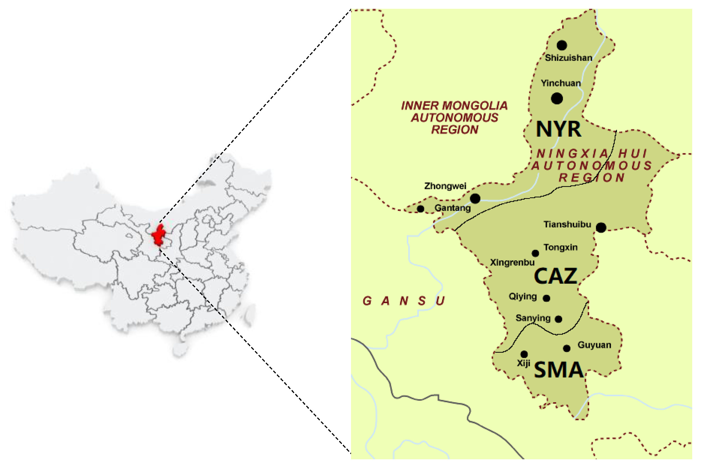
Ningxia is located in northwestern China. It is bordered by Shaanxi, Inner Mongolia, and Gansu. It has five prefecture-level cities, namely, Yinchuan, Shizuishan, Wuzhong, Guyuan, and Zhongwei. Ningxia is far from the ocean and is located inland, forming a more typical continental climate, with the characteristics of long winter coldness, short summer heat, warm spring, and early autumn; drought and little rainfall, sufficient sunshine, strong evaporation, wind, and sand; cool south and warm north, wet and dry south, and more meteorological disasters. The geographical location of the Ningxia Hui Autonomous Region on the map of China and the distribution of sites in the Ningxia area are shown in Figure 1. The red area on the left shows the geographical location of the Ningxia Hui Autonomous Region in China, and on the right is the distribution map of topographic and meteorological stations in the Ningxia Hui Autonomous Region.in the map. NYR represents the northern Yellow River, CAZ represents the central arid zone, and SMA represents the southern mountainous area. The three cities of Shizuishan, Yinchuan, and Zhongwei are distributed in NYR District, Wuzhong City is distributed in CAZ District, and Guyuan City is distributed in SMA District.
2.2. Sources and Data Presentation
This article uses day-to-day data of PM2.5, PM10, NO2, SO2, O3, and CO from 1 January 2018 to 31 December 2020 in five municipal districts of Ningxia from the website of the National Center for Environmental Information of the National Oceanic and Atmospheric Administration (NOAA—National Centers for Environmental Information, https://www.ncei.noaa.gov/ (accessed on 5 April 2021)). Day-by-day data are the result of arithmetic averaging based on hourly data. Near-surface conventional meteorological data are derived from the Copernicus Atmosphere Monitoring Service (EAC4-Copernicus Atmosphere Monitoring Service, https://ads.atmosphere.copernicus.eu/ (accessed on 10 April 2021)) global atmospheric composition reanalysis dataset, which includes the monitoring results of five stations in Ningxia, namely, Tongxin, Yinchuan, Zhongwei, Taole, and Guyuan. Table 1 shows the basic information of the five selected meteorological monitoring stations.
2.2.1. Statistical Analysis of Data
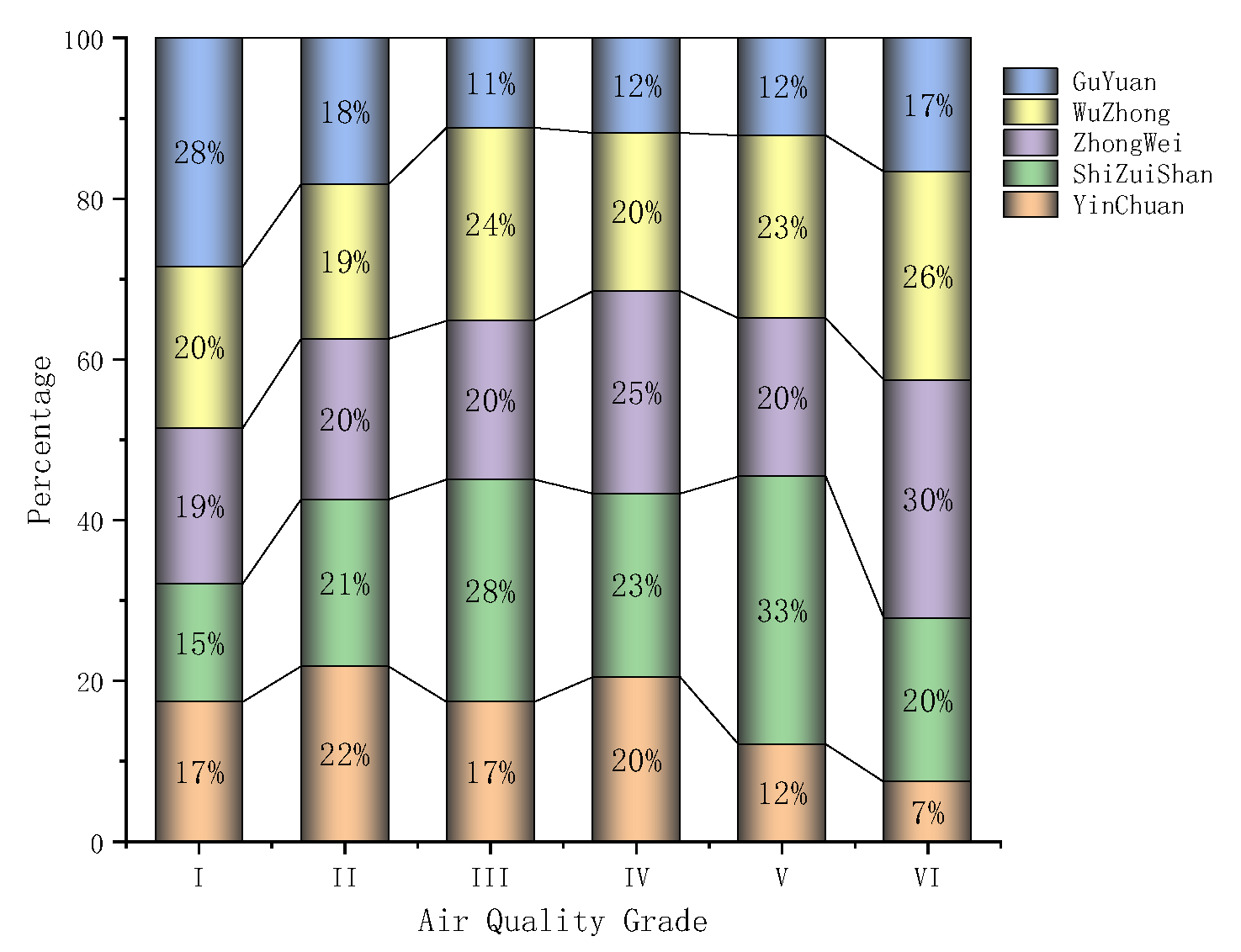
According to the new air quality standard of the PM2.5 testing network, the air quality is divided into six levels: excellent, good, light pollution, moderate pollution, heavy pollution, and serious pollution, by using the daily average concentration of PM2.5. The data were integrated, the proportion of air quality grades in five municipal areas were first counted, and the results shown in Figure 2 show that the concentration of Guyuan PM2.5 in 0–35 accounted for the largest proportion of 28.47%, followed by Wuzhong accounting for 20.1%, Zhongwei accounting for 19%, Yinchuan accounting for 17%, and Shizuishan accounting for the smallest 14.7%. The PM2.5 dataset was then statistically analyzed, and the results are shown in Table 2. The results showed that among the five cities, the average value of Shizuishan City was 40.26, followed by Wuzhong City at 35.39, Zhongwei City at 35.02, Yinchuan City at 33.90, and Guyuan City at 28.29; the minimum value of Guyuan City was 2, the maximum value was 169, and the standard deviation was 18.79. After a comprehensive comparison, the four statistical indicators of Guyuan City are significantly lower than those of the other four cities. In summary, the overall indicators of Guyuan are better than those of the other four cities, Shizuishan City is the worst, which has a clear correlation with the geographical location of the municipal area, and the overall air quality in the southern mountainous area is better than that in the northern Yellow River irrigation district.
2.2.2. Time Dimension Analysis of PM2.5 Concentration
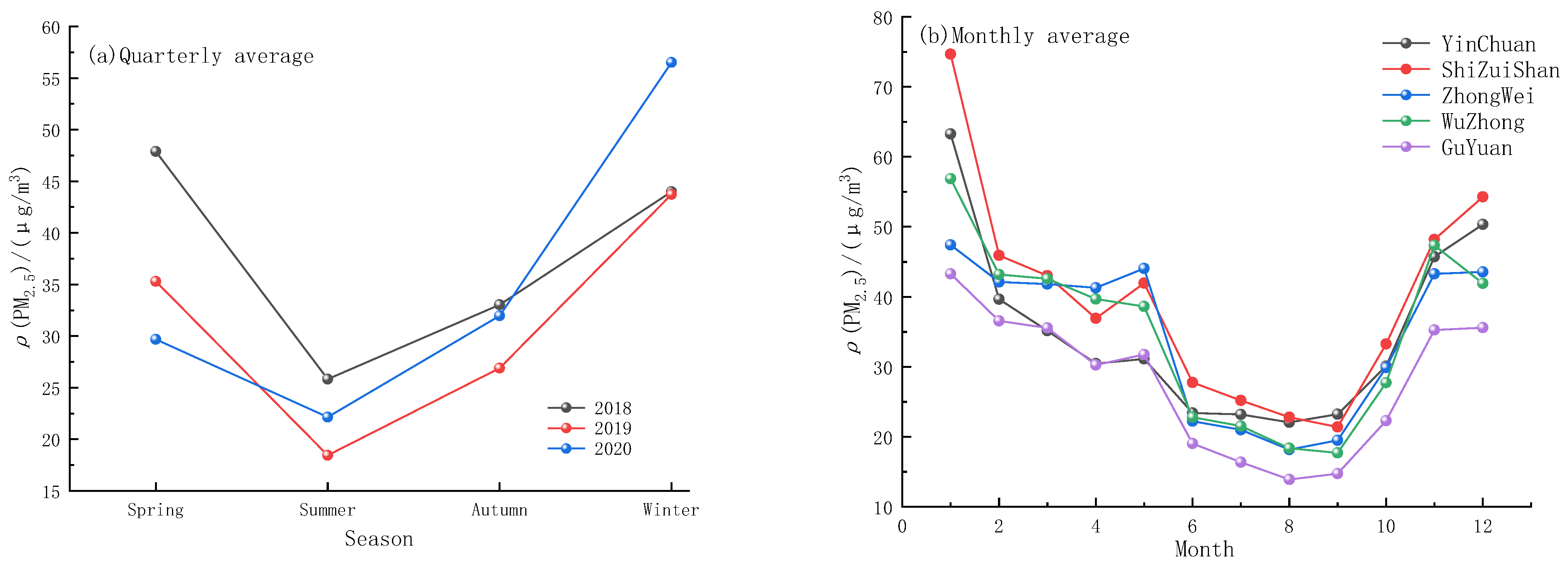
Based on the dataset from 2018 to 2020, the three-year data of the five cities are divided according to the four seasons of spring, summer, autumn, and winter. The three-year PM2.5 concentration data are divided into seasonal means and statistics, and the statistical results are shown in Figure 3a. It can be seen that PM2.5 concentration is the lowest in summer and the highest in winter. This suggests that the concentration of PM2.5 is affected by seasonal changes and may have some correlation with meteorological elements. Therefore, the addition of meteorological factor data can better predict the concentration of PM2.5.
The monthly statistics of PM2.5 concentration data in five cities from 2018 to 2020 were carried out. The average value of PM2.5 in each city in three years was calculated according to the month, and the statistical data were drawn as the line graph of Figure 3b. It was found that the monthly variation trend of PM2.5 concentration was obvious. A monthly downward trend began in January until the lowest in June–September, followed by a monthly upward trend from September. It further illustrates the seasonal variation of PM2.5 concentrations, with the lowest in summer and the highest in winter. First, since coal burning in winter is the main method of household heating and energy supply, this has a strong correlation with the soot emitted by coal and gas or fuel oil during the winter heating process in Ningxia. Secondly, the spring and winter periods in Ningxia have greater wind and sandstorms, and wind disasters and sandstorms are affected by the terrain; generally, there are more Yellow River irrigation areas in the north and fewer mountainous areas in the south. Wind and sand will increase the concentration of PM2.5 in the atmosphere and make the air quality worse.
2.2.3. Variable Correlation Analysis
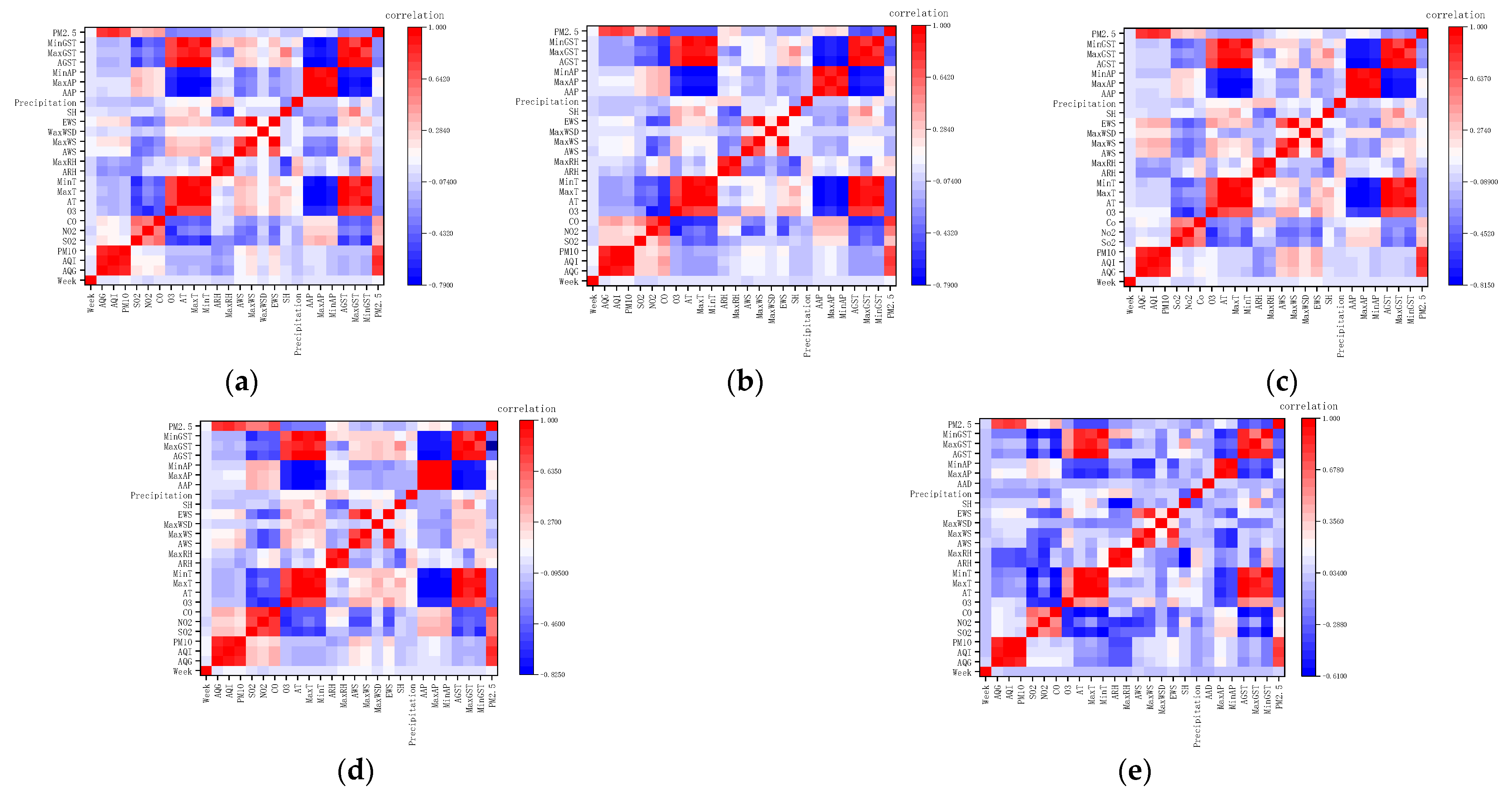
Variable correlation analysis was performed on the data of five municipal districts to obtain a heat map of the correlation coefficient shown in Figure 4. The results showed a strong positive correlation between air pollution level and PM2.5 concentration, and the correlation coefficient was 0.78. Four atmospheric pollutants, PM10, NO2, SO2, and CO, also had a strong positive correlation with PM2.5 concentrations, with correlation coefficients of 0.37 to 0.74. O3 was inversely correlated with PM2.5 concentrations, with a correlation coefficient of −0.32. In addition, there was an obvious negative correlation between surface air temperature and PM2.5 concentration among meteorological factors, and the correlation coefficient was −0.3~−0.35. There is a strong correlation between some input variables, and to eliminate the correlation effect between the variables, the experimental data need to be reduced by principal component analysis (PCA).
2.3. Data Preprocessing
2.3.1. Data Quality Control
The collected air pollutant data and meteorological factor data of the five cities are subjected to quality control; each feature is checked, and first of all, all data for that day need to be excluded for outliers that are not within the range of a feature value. Second, for the treatment of a feature missing value, it needs to be filled with the average of the two data values adjacent to the missing value. If the value adjacent to it does not exist, all data for that day need to be excluded. Through the quality control of the original 1095 days of data from 2018 to 2020 in five municipal areas, the data of 45 days were deleted and the remaining 1050 days of data were used for research. A total of 26 data on atmospheric pollutants and meteorological elements are available per day. Influencing factors are stated as follows: week, air quality grade (AQG), air quality index (AQI), average temperature (AT), maximum temperature (MaxT), minimum temperature (MinT), average relative humidity (ARH), maximum relative humidity (MaxRH), average wind speed (AWS), maximum wind speed (MaxWS), maximum wind speed (MaxWSD), maximum wind speed (EWS), hours of sunshine (SH), precipitation, average air pressure (AAP), maximum air pressure (MaxAP), minimum air pressure (MinAP), average surface temperature (AGST), maximum surface temperature (MaxGST), and minimum surface temperature (MinGST).
2.3.2. Data Normalization and Data Segmentation
In order to avoid dimensional differences between various factors, this paper uses min–max normalization for data normalization, and the specific functions are as follows:
where is the maximum number in the data series and is the smallest number in the data series. The dataset is then divided into 850 days of data to train the model as a training set and 200 days of data to test the model as a test set.
3. Research Methodology
3.1. Experimental Process and Evaluation Method
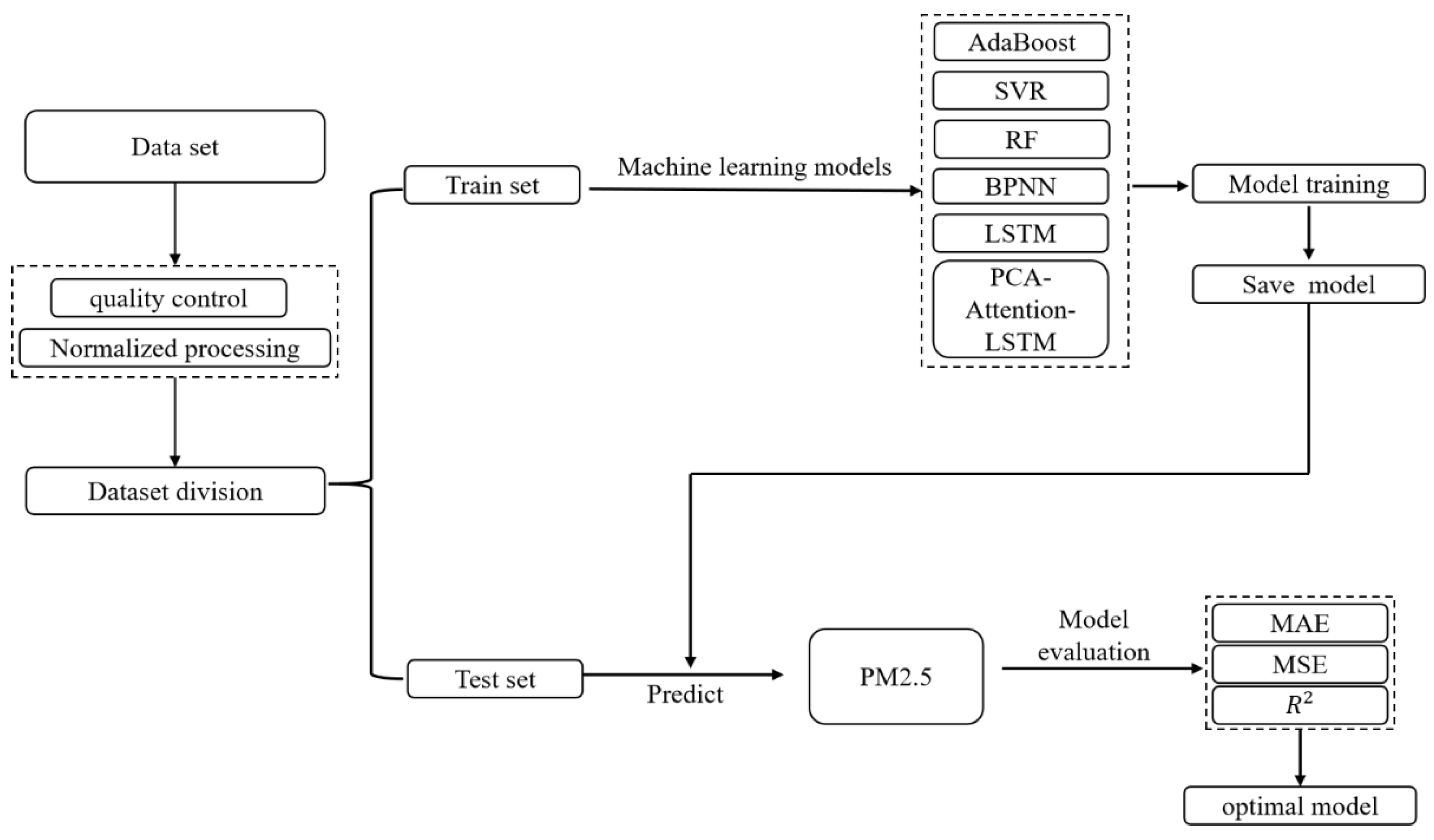
The experimental process of predicting PM2.5 concentration is shown in Figure 5, including data preprocessing, model construction, model prediction, and analysis. Firstly, the experimental data are preprocessed and normalized, and the data are divided into training set and test set. Secondly, the training set is used to train multiple machine learning models and save them. Finally, the prediction values of each model for PM2.5 concentration are obtained by the test set, and the experimental results are compared and analyzed by the evaluation method. The specific process is as follows:
In this paper, three model evaluation methods were adopted for the statistical testing index: correlation coefficient (), mean absolute error (MAE), and mean squared error (MSE). The calculation method of each indicator is as follows:
where is the simulated value, is the observed value, and is the observed mean.
3.2. Machine Learning Methods
The random forest model (RF) is a bagging method, which draws multiple samples from the dataset randomly placed back at a set feature ratio, then trains each sample by returning to the tree, and finally adopts a combined strategy for the prediction results obtained by each tree, then obtains the prediction results of the final random forest model [17,18,19].
The support vector machine (SVM) uses the SMO or gradient descent method to solve the parameters in the Lagrange dual function, and then finds the optimal classification decision boundary. Generalized support vector regression (SVR) models can be used to solve regression problems; SVR models find a regression plane so that the data sample is closest to the regression plane, thereby obtaining the predicted value [20,21,22,23].
The AdaBoost model improves model accuracy by automatically adjusting the weights of each round. The model learns a weak classifier at a time by iterating and changing the weights of each data in each iteration. The weak classifiers are then linearly combined to obtain a strong classifier.
The BP neural network model (BPNN) is an iterative form, first using the forward propagation of the signal to obtain the results of the first training, and then, according to the error of the ideal and actual output, the signal is backpropagation, so that the process of learning and training is learned and trained through continuous propagation and adjustment of model parameters [24,25]. The input layer of the neural network in this paper is the air pollutant data and meteorological feature data, the activation function of the implicit layer is the sigmoid function, and the output layer is the predicted value of PM2.5.
3.3. PCA-Attention-LSTM
3.3.1. Principal Component Analysis (PCA)
PCA transforms multiple indexes into several comprehensive indexes, and the transformed comprehensive indexes are transformed into principal components. The principal components are not correlated with each other, which simplifies the research problem and improves the analysis efficiency.
The total number of indicators studied in this paper is , which are represented by , each prefecture-level city has samples, and the jth indicator of the ith sample takes the value of , converting into a standardized indicator ,
where , , i.e., and are the sample mean and standard deviation of the jth indicator, respectively. Correspondingly, is called a standardized indicator variable.
Correlation coefficient matrix , where is the correlation coefficient between the ith indicator and the jth indicator. We calculate the eigenvalue of the correlation coefficient matrix R, and the corresponding eigenvector , where , consists of a new indicator variable m by the eigenvectors
where is the 1st principal component, is the 2nd principal component, and is the m principal component. Calculate the information contribution rate and cumulative contribution rate of the eigenvalue . is the information contribution rate of the jth principal component; is the cumulative contribution rate of the principal component , AP = 85~90% is selected, the number of p main components is selected, and the p comprehensive variable replaces the original m initial index. We bring p synthesis metrics into the BP neural network model. We bring p synthesis metrics into the long short-term memory neural networks that incorporate attention mechanisms.
3.3.2. Long Short-Term Memory Neural Network (LSTM)
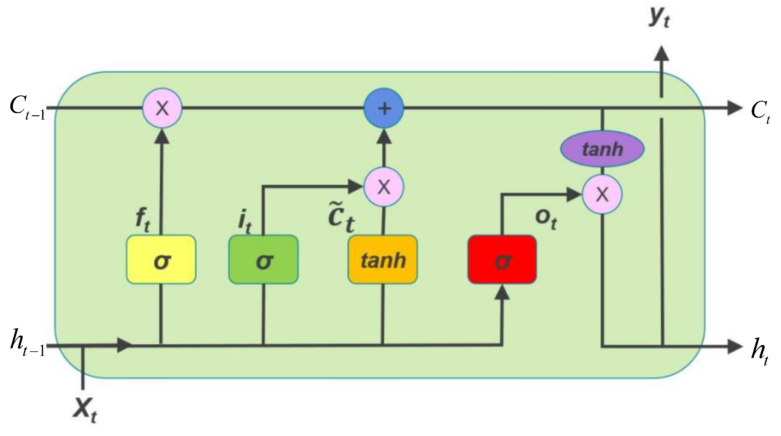
Recurrent neural network (RNN) is a neural network for processing sequence data, and long short-term memory neural network (LSTM) is a special kind of RNN, mainly used to solve the gradient disappearance and gradient explosion problems in the long sequence training process. Compared to ordinary RNNs, in longer sequence, LSTM has better performance. On the basis of the original RNN, LSTM adds an additional unit that can save the long-term state in the hidden layer, and the internal structure of the LSTM unit is shown in Figure 6. LSTM and GRU are special RNN architectures used to solve the gradient vanishing problem. GRU can be considered a simplified version of LSTM. The performances of GRU and LSTM are indistinguishable in many tasks. The fewer GRU parameters make it easier to converge, but LSTM has better expression performance when the dataset is large. After comprehensive consideration, LSTM is selected as the main algorithm for predicting PM2.5 concentration in this paper. At the top of Figure 6 is a long-term memory C line that runs horizontally to achieve the purpose of sequence learning. Three neural network layers represent three doors.
The forgetting gate determines the retention of past information by judging the importance of the current input information, the gate reads ht−1, Xt−1, outputs a value between 0 and 1 to each number in the cell state Ct−1, 1 means complete retention, 0 means complete discard.
The input gate determines the retention of the input information by judging the importance of the current input information, which determines how much new information is added to the cell state, a sigmoid layer determines that the information needs to be updated, and a tanh layer generates a vector, that is, the alternative content used to update, merging the two parts to update the cell state. The output gate runs a sigmoid layer to determine the part of the cell state that will be exported, and then the cell state is processed by tanh to obtain a value between −1 and 1, and it is multiplied by the output of the sigmoid gate to obtain the output result. The symbols in the figure are calculated as follows:
where ht−1 represents the output of the previous cell; xt represents the input of the current cell; σ represents sigmod function; ct−1 is the output of the previous moment; ct is the output of the current moment; ft is the output of forgetting gate; ot is the output of the output gate; is an alternative content for updating; it is the update degree of input gate; ht is the current cell output.
3.3.3. Attention Mechanism
The essence of the attention mechanism is the mental activity of the brain when people observe things. When the brain sees something important that often appears in one part of a scene, it will learn and then focus on this part when it sees a similar scene. In the actual application process, the standard LSTM cannot be handled well in the face of multidimensional and multivariable datasets, and some important time series information may be ignored during the model training process, which will affect the accuracy of the model. Therefore, attention mechanism is added on the basis of LSTM in order to better judge the importance of information at each input moment. Attention mechanism gives different weights to the input characteristics of LSTM, highlights the key influencing factors, and improves the prediction accuracy of the model without increasing the calculation and storage space of the model.
The attention model uses the attention mechanism to dynamically generate the weights of different connections between the input and output of the same layer of network to obtain the output model of the network. The self-attention model can be used as a layer of the neural network, it can also be used to replace the convolution layer or loop layer, or it can be cross-stacked with the convolution layer or loop layer. The mathematical formula is used to express the self-attention mechanism. Assuming that the input sequence in a nerve layer is , and the output sequence is with the same length, three groups of vector sequences are obtained through linear transformation. is the query vector sequence, is the key vector sequence, and is the value vector sequence.
where ,, are learnable parameter matrices. We calculate the output vector:
where is the position of the output and input vector sequence, the connection weight is dynamically generated by the attention mechanism.
3.3.4. PCA-Attention-LSTM Forecasting Model
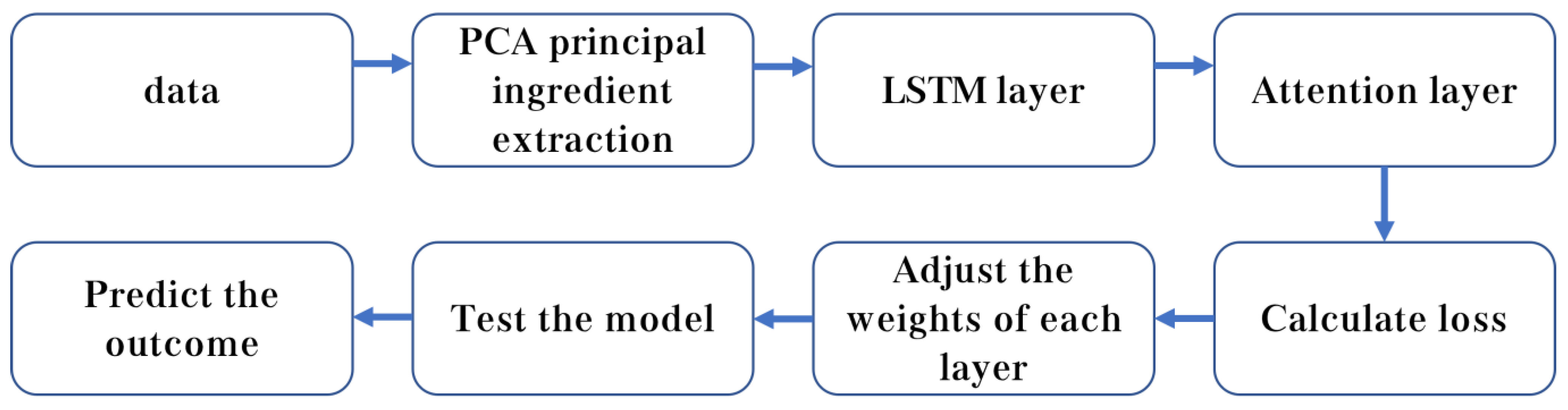
LSTM solves the problem of gradient disappearance and gradient explosion during long sequence training very well. PCA is used to reduce the dimensionality of the data to speed up the training speed of the model with the smallest amount of lost information. Adding the attention mechanism can better capture important features of long time series data. The model adopts the keras deep learning framework architecture network model, integrates the three algorithms of PCA, attention mechanism, and LSTM, and establishes an LSTM model based on PCA and attention mechanism; the model framework is shown in Figure 7.
4. Experimental Results and Analysis
4.1. PCA-Attention-LSTM Model Building Results
According to the cumulative contribution rate of 85% to 90%, the number of principal components corresponding to the data of the five prefecture-level cities in Ningxia was determined, and the results are shown in Table 3. Wuzhong and Gu Yuan selected eight main components, and Yinchuan, Zhongwei, and Shizuishan selected seven main components. This turns the original 26 indicators into seven or eight comprehensive indicators, so that while eliminating the influence of correlation between variables, the complexity of the model can be reduced and the operation speed of the model can be improved. In the process of the simulation experiment, the principal components are input into the LSTM neural network based on the attention mechanism to build a PCA-attention-LSTM model. The number of principal components selected in the five regions of this paper is seven or eight, and the specific results are shown in Table 3.
4.2. Model Parameter Selection
Adaboost model parameters are base_estimator = None, n_estimators = 56, learning_rate = 0.1, algorithm = SAMME.R, random_state = None. SVR model parameters are kernel = rbf, gamma = scale, tol = 0.001, C = 1.1, epsilon = 0.08, shrinking = True, cache_size = 200, verbose = False, max_iter = −1. RF model parameters estimator = rf, n_iter = 100, score = “neg_mean_absolute_error”, cv = 3, random_state = 42, n_jobs = −1, param_distribution = random_grid. The parameters of BPNN model are num_iterations = 1000, learning_rate = 0.01, n_h = 6, correct = 0.1. LSTM model parameters are time_step = 20, rnn_unit = 10, batch_size = 60, input_size = 26, output_size = 1, lr = 0.006. In the PCA-attention-LSTM model, the LSTM layer activation function is sigmoid, full connection layer node number is 4, full connection layer node learning rate is 0.005, and full connection layer activation function is sigmoid.
4.3. Model Prediction Results and Comparisons
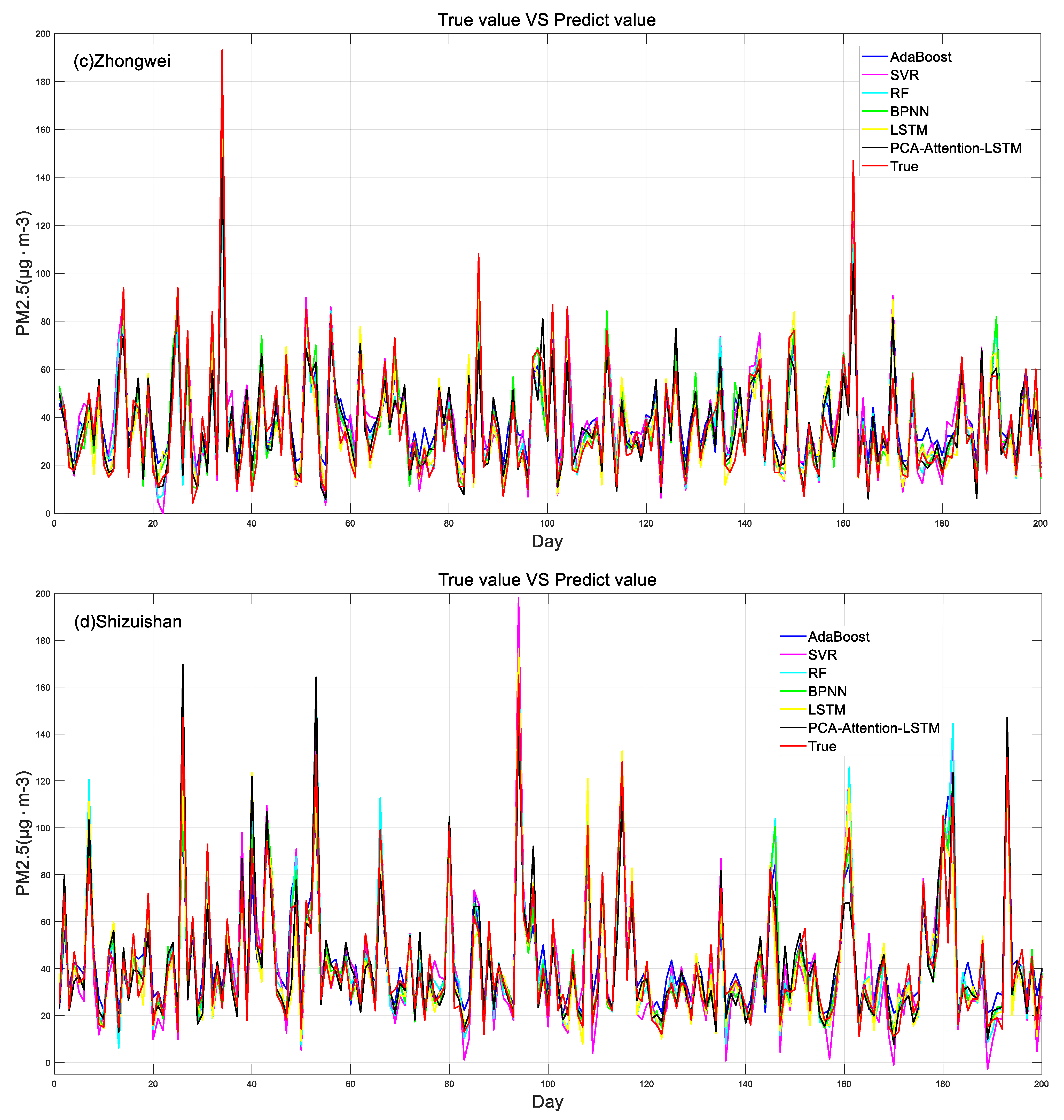
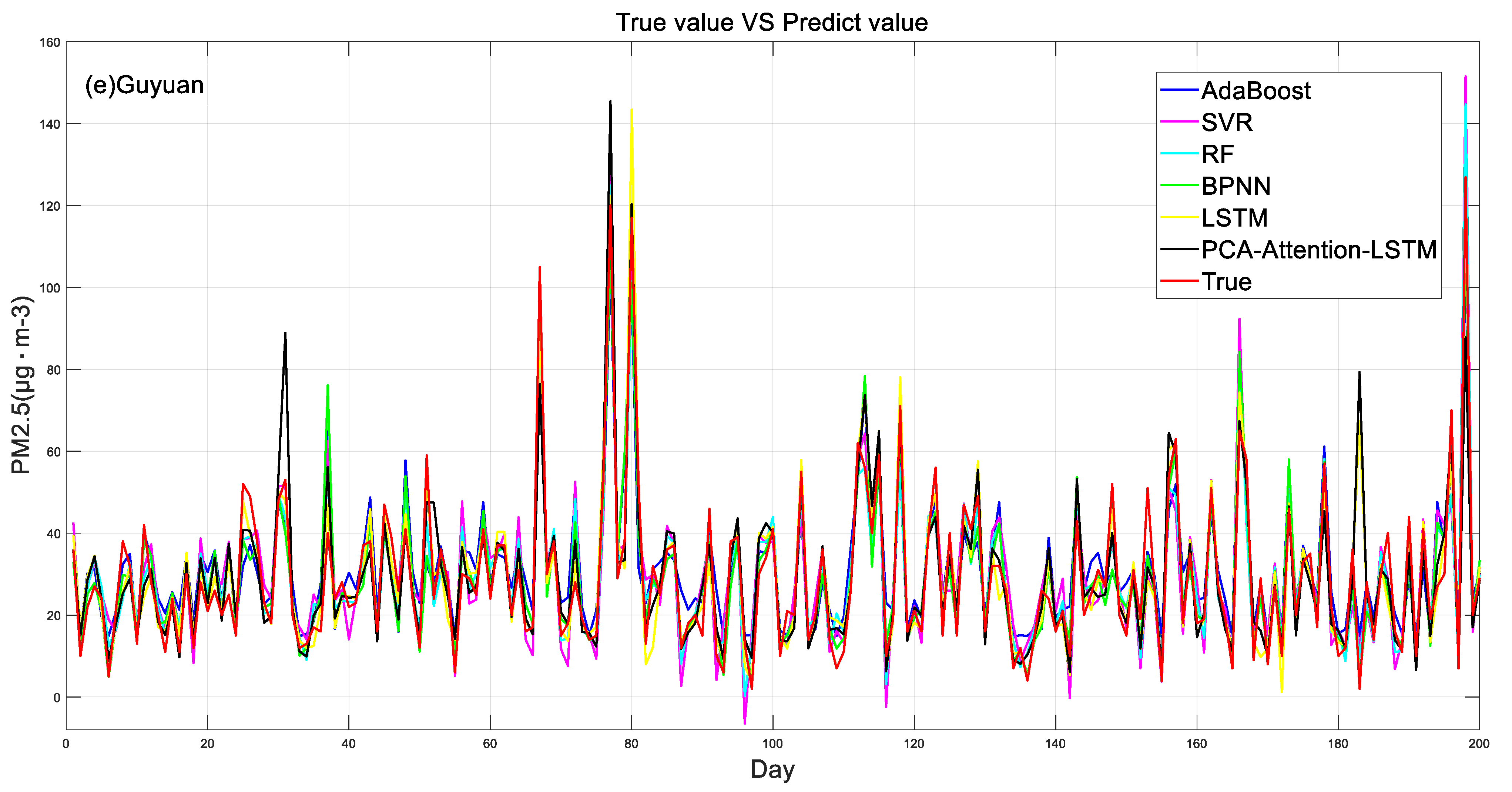
Experiments were conducted using data of the five municipal districts to obtain a line chart of the measured and predicted values of PM2.5 in the five municipal areas, as shown in Figure 8. Three model evaluation methods, R2, MAE, and MSE, were used to analyze the prediction accuracy of the models. The results are shown in Table 4. The correlation coefficient (R2) values for the six models ranged from 0.75 to 0.93. The results showed that Wuzhong, Yinchuan, Zhongwei, Shizuishan, and Guyuan all adopted the PCA-attention-LSTM model as the best, and the correlation coefficients R2 were 0.91, 0.93, 0.91, 0.91, and 0.90, respectively, followed by the LSTM model, with the correlation coefficients R2 of 0.87, 0.91, 0.99, 0.99, 0.99, and 0.87, respectively, and the SVR model was the worst, with the correlation coefficients R2 of 0.75, 0.79, 0.83, and 0.79, respectively.
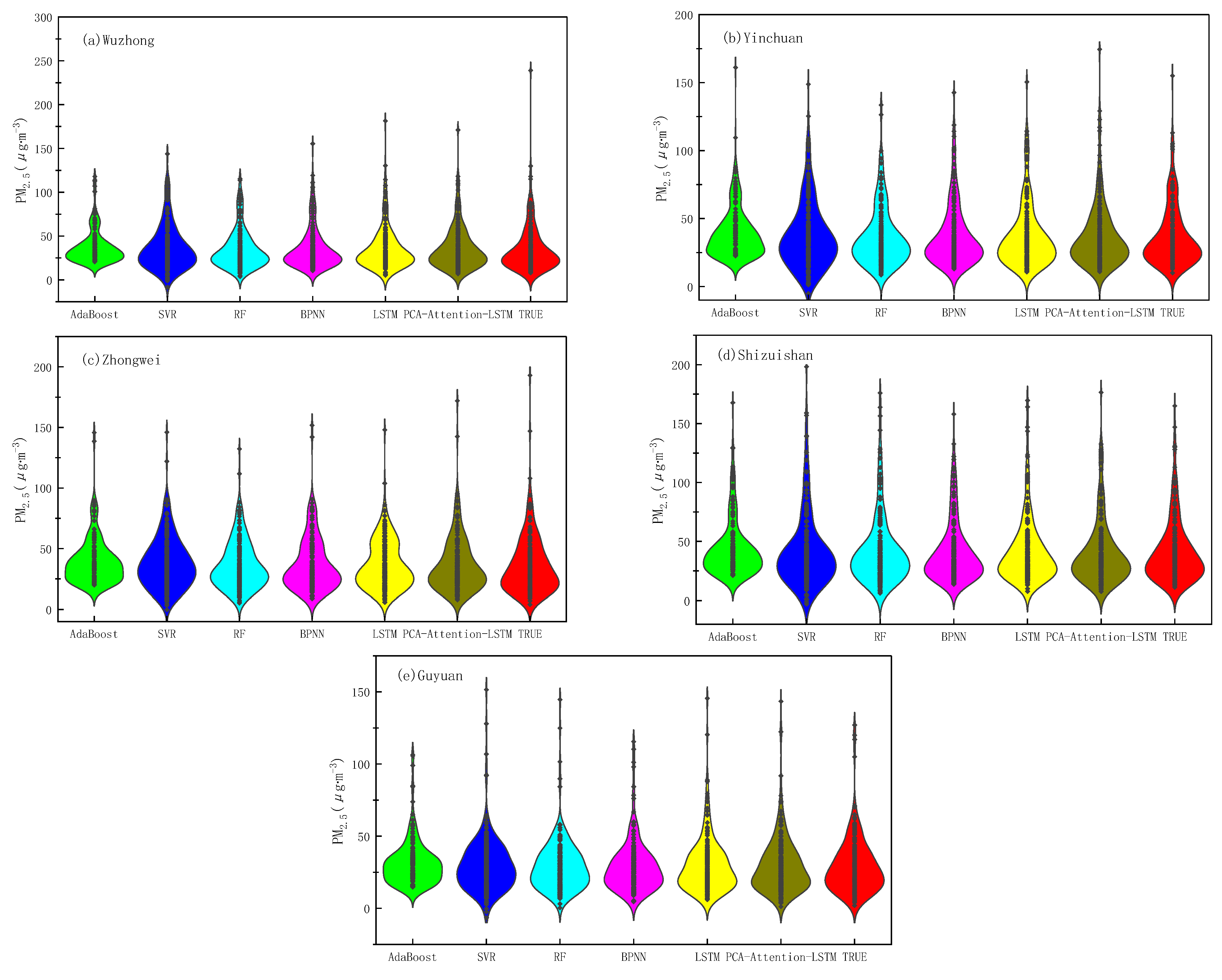
In order to further compare the relationship between the predicted values and the measured values of the six models, Figure 9 compares the true values of PM2.5 concentrations in five municipal areas with the predicted values of the models. It can be seen from Figure 9 that the AdaBoost model in the Wuzhong area as a whole shows an overestimation phenomenon, SVR and RF show an underestimation phenomenon, and the distribution of the PCA-attention-LSTM model and true values is the closest, but the peak is underestimated. The AdaBoost model in Yinchuan showed an overall overestimation phenomenon, the SVR showed an underestimation phenomenon, and the PCA-attention-LSTM model and the LSTM model were close to the distribution of the measured values. The LSTM model, BPNN model, and AdaBoost model in Zhongwei area showed an overall overestimation phenomenon, the RF model showed an underestimation phenomenon, and the PCA-attention-LSTM model was close to the overall distribution of the measured values but the peak was underestimated. The Shizuishan area and the AdaBoost model as a whole showed an overestimation phenomenon, the SVR and RF models showed an underestimation phenomenon, and the range of predicted values became larger, and the PCA-attention-LSTM model and LSTM model were close to the overall distribution of the measured values. The AdaBoost model in the Guyuan area showed an overall overestimation phenomenon, and the PCA-attention-LSTM model was closest to the overall distribution of the measured values.
5. Conclusions and Discussions
- (1)
- Statistical analysis of the data shows that the overall indicators of Guyuan are better than those of the other four cities, and the worst is Shizuishan City, which has a clear correlation with the geographical location of the municipal areas, and the overall air quality in the southern mountainous areas is better than that of the Yellow River irrigation area in the north.
- (2)
- The three-year data of five cities in Ningxia were integrated and divided into four seasons and month by month. The results showed that the PM2.5 concentration showed an obvious seasonal change trend, which was the lowest in summer and the highest in winter. This was mainly related to the dust emission from coal combustion and gas or fuel during winter heating in Ningxia.
- (3)
- Through the analysis of variable importance, the results show that PM10 is the most important, followed by air quality index, air quality grade, and CO having equal importance, and precipitation in meteorological elements is also a relatively important variable. For future studies of PM2.5 concentration prediction, the week can also be used as an input variable, indicating that PM2.5 concentration generation is also affected by weekdays and non-working days.
- (4)
- The concentration of PM2.5 was predicted by using six models, and the results showed that the PCA-attention-LSTM model had the best prediction accuracy, and its correlation coefficient was 0.91~0.93. The prediction accuracy of the SVR model was poor, and its correlation coefficient was 0.75~0.83. The LSTM model and the BPNN model also predicted better results.
- (5)
- Experimental results show that the training evaluation results of the PCA-attention-LSTM model are better than those of the LSTM model, which shows that the cumulative variance contribution rate of the selected principal components reaches 85–90%, which reduces the data dimension and reduces the time complexity and spatial complexity of the model. At the same time, the attention mechanism can better capture important information.
Author Contributions
Conceptualization, methodology, resources, writing—review and editing, supervision, project administration, funding acquisition, W.D. software, validation, formal analysis, investigation, data curation, writing—original draft preparation, visualization, Y.Z. All authors have read and agreed to the published version of the manuscript.
Funding
This work was supported by the Ningxia Natural Science Foundation under Grant no. 2021AAC03223, the National Natural Science Foundation of China under Grant no. 11761002, First Class Disciplines Foundation of Ningxia under Grant NXYLXK2017B09, Western light project of Chinese Academy of Sciences: Application of big data analysis technology in air pollution assessment.
Institutional Review Board Statement
Not applicable.
Informed Consent Statement
Not applicable.
Data Availability Statement
Not applicable.
Conflicts of Interest
The authors declare no conflict of interest.
References
- Liu, Y.; Zhou, Y.; Lu, J. Exploring the relationship between air pollution and meteorological conditions in China under environ-mental governance. Nat. Res. Sci. Rep. 2020, 10, 14518. [Google Scholar] [CrossRef] [PubMed]
- Ding, W.; Zhang, J.; Leung, Y. A hierarchical Bayesian model for the analysis of space-time air pollutant concentrations and an application to air pollution analysis in Northern China. Stoch. Environ. Res. Risk Assess. 2021, 35, 2237–2271. [Google Scholar] [CrossRef]
- Ding, W.; Zhang, J. Prediction of Air Pollutants Concentration Based on an Extreme Learning Machine: The Case of Hong Kong. Int. J. Environ. Res. Public Health 2017, 14, 114. [Google Scholar]
- Ding, W.; Zhang, J.; Leung, Y. Prediction of air pollutant concentration based on sparse response back-propagation training feedforward neural networks. Environ. Sci. Pollut. Res. 2016, 23, 19481–19494. [Google Scholar] [CrossRef]
- Bell, M.; Ebisu, K.; Dominici, F. Spatial and temporal variation in PM2.5 chemical composition in the United States. Palaeontology 2006, 58, 133–140. [Google Scholar] [CrossRef]
- Qin, W.; Zhang, Y.; Chen, J.; Yu, Q.; Cheng, S.; Li, W.; Liu, X.; Tian, H. Variation, sources and historical trend of black carbon in Beijing, China based on ground observation and MERRA-2reanalysis data. Environ. Pollut. 2019, 245, 853–863. [Google Scholar] [CrossRef]
- Liag, M.; Wang, L.; Liu, J.; Gao, W.; Song, T.; Sun, Y.; Li, L.; Li, X.; Wang, Y.; Liu, L.; et al. Exploring the regional pollution characteristics and meteorological formation mechanism of PM2.5 in North China during 2013–2017. Environ. Int. 2020, 134, 105283. [Google Scholar]
- Jin, J.; Du, Y.; Xu, L.; Chen, Z.; Chen, J.; Wu, Y.; Ou, C. Using Bayesian spatio-temporal model to determine the socio-economic and meteorological factors influencing ambient PM2.5 levels in 109 Chinese cities. Environ. Pollut. 2019, 254, 113023. [Google Scholar] [CrossRef]
- Chen, B.; Lin, Y.; Deng, J.; Li, Z.; Dong, L.; Huang, Y.; Wang, K. Spatiotemporal dynamics and exposure analysis of daily PM2.5 using a remote sensing-based machine learning model and multi-time meteorological parameters. Atmos. Pollut. Res. 2021, 12, 23–31. [Google Scholar] [CrossRef]
- Rybarczyk, Y.; Zalakeviciute, R. Machine learning approach to forecasting urban pollution: A case study of Quito. In Proceedings of the IEEE Ecuador Technical Chapters Meeting, (ETCM’16), Guayaquil, Ecuador, 12–14 October 2016. [Google Scholar]
- Wang, J.; Ogawa, S. Effects of meteorological conditions on PM2.5 concentrations in Nagasaki, Japan. Int. J. Environ. Res. Public Health 2015, 12, 9089–9101. [Google Scholar] [CrossRef]
- Jimenez, P.A.; Dudhia, J. Improving the representation of resolved and unresolved topographic effects on surface wind in the WRF model. J. Appl. Meteorol. Climatol. 2012, 51, 300–316. [Google Scholar] [CrossRef]
- Ni, X.; Huang, H.; Du, W. Relevance analysis and short-term prediction of PM2.5 concentrations in Beijing based on multi-source data. Atmos. Environ. 2017, 150, 146–161. [Google Scholar] [CrossRef]
- Brokamp, C.; Jandarov, R.; Hossain, M.; Ryan, P. Predicting daily urban fine particulate matter Concentrations using a random forest model. Environ. Sci. Technol. 2018, 52, 4173–4179. [Google Scholar] [CrossRef]
- Zhao, R.; Gu, X.X.; Xue, B.; Zhang, J.Q.; Ren, W.X. Short period PM2.5 prediction based on multivariate linear regression model. PLoS ONE 2018, 13, e0201011. [Google Scholar] [CrossRef]
- Akbal, Y.; Ünlü, K.D. A deep learning approach to model daily particular matter of Ankara: Key features and forecasting. Int. J. Environ. Sci. Technol. 2021, 19, 5911–5927. [Google Scholar] [CrossRef]
- Brokamp, C.; Jandarov, R.; Rao, M.B.; LeMasters, G.; Ryan, P. Exposure assessment models for elemental components of particulate matter in an urban environment: A comparison of regression and random forest approaches. Atmos. Environ. 2017, 151, 1–11. [Google Scholar] [CrossRef]
- Russo, A.; Raischel, F.; Lind, P.G. Air quality prediction using optimal neural networks with stochastic variables. Atmos. Environ. 2013, 79, 822–830. [Google Scholar] [CrossRef]
- Singh, K.P.; Gupta, S.; Rai, P. Identifying pollution sources and predicting urban air quality using ensemble learning methods. Atmos. Environ. 2013, 80, 426–437. [Google Scholar] [CrossRef]
- Karimian, H.; Li, Q.; Wu, C.; Qi, Y.; Mo, Y.; Chen, G.; Zhang, X.; Sachdeva, S. Evaluation of different machine learning approaches to forecasting PM2.5 mass concentrations. Aerosol Air Qual. Res. 2019, 19, 1400–1410. [Google Scholar] [CrossRef]
- Osowski, S.; Garanty, K. Engineering Applications of Artificial Intelligence. Eng. Appl. Artif. Intell. 2007, 20, 745–755. [Google Scholar] [CrossRef]
- Yoon, H.; Jun, S.-C.; Hyun, Y.; Bae, G.-O.; Lee, K.-K. A comparative study of artificial neural networks and support vector machines for predicting groundwater levels in a coastal aquifer. J. Hydrol. 2011, 396, 128–138. [Google Scholar] [CrossRef]
- Song, L.; Pang, S.; Longley, I.; Olivares, G.; Sarrafzadeh, A. Spatio-temporal PM 2.5 prediction by spatial data aided incremental support vector regression. In Proceedings of the IEEE International Joint Conference on Neural Networks (IJCNN), Beijing, China, 6–11 July 2014; pp. 623–630. [Google Scholar]
- Arhami, M.; Kamali, N.; Rajabi, M.M. Predicting hourly air pollutant levels using artificial neural networks coupled with uncertainty analysis by Monte Carlo simulations. Environ. Sci. Pollut. Res. 2013, 20, 4777–4789. [Google Scholar] [CrossRef]
- Zheng, H.; Shang, X. Study on prediction of atmospheric PM2.5 based on RBF neural network. In Proceedings of the IEEE Fourth International Conference on Digital Manufacturing and Automation (ICDMA), Qindao, China, 29–30 June 2013; pp. 1287–1289. [Google Scholar]
Figure 1.
China Ningxia regional division and site distribution.

Figure 2.
Five cities’ AQI grade percentage stacked chart.

Figure 3.
Statistics of seasonal and monthly mean value of PM2.5 concentration. (a) Seasonal mean statistics of PM2.5 concentration from 2018 to 2020; (b) Monthly mean statistics of PM2.5 concentration in 5 cities.
Figure 3.
Statistics of seasonal and monthly mean value of PM2.5 concentration. (a) Seasonal mean statistics of PM2.5 concentration from 2018 to 2020; (b) Monthly mean statistics of PM2.5 concentration in 5 cities.

Figure 4.
Correlation coefficient heat plot. (a) Wuzhong; (b) Yinchuan; (c) Zhongwei; (d) Shizuishan; (e) Guyuan.
Figure 4.
Correlation coefficient heat plot. (a) Wuzhong; (b) Yinchuan; (c) Zhongwei; (d) Shizuishan; (e) Guyuan.

Figure 5.
Experimental flow chart.

Figure 6.
LSTM unit internal structure diagram.

Figure 7.
PCA-attention-LSTM model technical roadmap.

Figure 8.
True value versus predicted value.


Figure 9.
A plot of the distribution of predicted and true values.


Table 1.
Basic information of each monitoring station in Ningxia.
| Site Number | Monitor the Site Name | Municipal Level | Longitude | Latitude | Elevation (m) |
|---|---|---|---|---|---|
| 53614 | Yinchuan | Yinchuan City | 106°12′ | 38°28′ | 1110.9 |
| 53615 | Taole | Shizuishan City | 106°42′ | 38°48′ | 1101.6 |
| 53704 | Zhongwei | Zhongwei City | 105°11′ | 37°32′ | 1226.7 |
| 53810 | Tongxin | Wuzhong City | 105°54′ | 36°58′ | 1336.4 |
| 53817 | Guyuan | Guyuan City | 106°16′ | 36°00′ | 1752.8 |
Table 2.
The main statistical indicators of PM2.5 in air quality monitoring stations.
| Statistical Indicators | Yinchuan | Shizuishan | Zhongwei | Wuzhong | Guyuan |
|---|---|---|---|---|---|
| Minimum (µg m−3) | 9 | 8 | 4 | 4 | 2 |
| Maximum (µg m−3) | 240 | 207 | 217 | 239 | 169 |
| average value (µg m−3) | 33.90 | 40.26 | 35.02 | 35.39 | 28.29 |
| standard deviation | 20.90 | 28.03 | 24.61 | 26.16 | 18.79 |
Table 3.
Principal component analysis.
| City | Principal Component | Eigenvalue | Contribution Rate % | Cumulative Contribution Rate % |
|---|---|---|---|---|
| Wuzhong | 1 | 3.0824 | 0.3800 | 0.3800 |
| 2 | 1.8978 | 0.1441 | 0.5241 | |
| 3 | 1.6590 | 0.1101 | 0.6342 | |
| 4 | 1.4086 | 0.0794 | 0.7136 | |
| 5 | 1.1236 | 0.0505 | 0.7640 | |
| 6 | 1.0012 | 0.0401 | 0.8041 | |
| 7 | 0.9901 | 0.0392 | 0.8434 | |
| 8 | 0.9293 | 0.0345 | 0.8779 | |
| Yinchuan | 1 | 3.1003 | 0.3845 | 0.3845 |
| 2 | 1.8770 | 0.1409 | 0.5254 | |
| 3 | 1.6928 | 0.1146 | 0.6400 | |
| 4 | 1.4783 | 0.0874 | 0.7274 | |
| 5 | 1.0550 | 0.0445 | 0.7720 | |
| 6 | 1.0200 | 0.0416 | 0.8136 | |
| 7 | 0.9766 | 0.0381 | 0.8518 | |
| Zhongwei | 1 | 3.0270 | 0.3665 | 0.3665 |
| 2 | 2.0319 | 0.1651 | 0.5317 | |
| 3 | 1.6637 | 0.1107 | 0.6424 | |
| 4 | 1.4807 | 0.0877 | 0.7301 | |
| 5 | 1.1071 | 0.0490 | 0.7791 | |
| 6 | 0.9926 | 0.0394 | 0.8185 | |
| 7 | 0.9313 | 0.0347 | 0.8532 | |
| Shizuishan | 1 | 3.1661 | 0.4010 | 0.4010 |
| 2 | 1.9037 | 0.1450 | 0.5460 | |
| 3 | 1.6964 | 0.1151 | 0.6611 | |
| 4 | 1.5811 | 0.1000 | 0.7610 | |
| 5 | 1.0097 | 0.0408 | 0.8018 | |
| 6 | 0.9549 | 0.0365 | 0.8383 | |
| 7 | 0.9472 | 0.0359 | 0.8742 | |
| Guyuan | 1 | 2.7533 | 0.3032 | 0.3032 |
| 2 | 1.9831 | 0.1573 | 0.4605 | |
| 3 | 1.8137 | 0.1316 | 0.5921 | |
| 4 | 1.4256 | 0.0813 | 0.6734 | |
| 5 | 1.1952 | 0.0571 | 0.7305 | |
| 6 | 1.0271 | 0.0422 | 0.7727 | |
| 7 | 1.0165 | 0.0413 | 0.8141 | |
| 8 | 0.9750 | 0.0380 | 0.8521 |
Table 4.
Model evaluation results.
| City | Evaluation Methods | BPNN | SVR | RF | AdaBoost | LSTM | PCA-Attention-LSTM |
|---|---|---|---|---|---|---|---|
| Wuzhong | R2 | 0.81 | 0.75 | 0.78 | 0.77 | 0.87 | 0.91 |
| MAE | 6.47 | 9.61 | 6.67 | 8.32 | 5.79 | 5.57 | |
| MSE | 140.61 | 181.92 | 157.82 | 167.86 | 97.17 | 78.49 | |
| Yinchuan | R2 | 0.90 | 0.79 | 0.89 | 0.87 | 0.91 | 0.93 |
| MAE | 4.85 | 8.12 | 5.10 | 6.50 | 4.35 | 4.07 | |
| MSE | 54.15 | 107,34 | 56.01 | 64.15 | 43.57 | 39.59 | |
| Zhongwei | R2 | 0.88 | 0.81 | 0.84 | 0.84 | 0.89 | 0.91 |
| MAE | 6.52 | 7.77 | 6.67 | 7.86 | 5.64 | 5.40 | |
| MSE | 96.12 | 111.58 | 97.41 | 93.45 | 68.02 | 54.64 | |
| Shizuishan | R2 | 0.89 | 0.83 | 0.89 | 0.87 | 0.90 | 0.91 |
| MAE | 5.98 | 8.11 | 6.08 | 6.95 | 5.28 | 4.92 | |
| MSE | 86.96 | 101.03 | 89.42 | 96.84 | 64.30 | 67.81 | |
| Guyuan | R2 | 0.87 | 0.79 | 0.85 | 0.81 | 0.87 | 0. 90 |
| MAE | 5.23 | 6.35 | 5.29 | 7.05 | 4.89 | 4.72 | |
| MSE | 59.31 | 69.91 | 62.01 | 78.32 | 57.81 | 50.22 |
Publisher’s Note: MDPI stays neutral with regard to jurisdictional claims in published maps and institutional affiliations. |
© 2022 by the authors. Licensee MDPI, Basel, Switzerland. This article is an open access article distributed under the terms and conditions of the Creative Commons Attribution (CC BY) license (https://creativecommons.org/licenses/by/4.0/).
Share and Cite
MDPI and ACS Style
Ding, W.; Zhu, Y. Prediction of PM2.5 Concentration in Ningxia Hui Autonomous Region Based on PCA-Attention-LSTM. Atmosphere 2022, 13, 1444. https://doi.org/10.3390/atmos13091444
AMA Style
Ding W, Zhu Y. Prediction of PM2.5 Concentration in Ningxia Hui Autonomous Region Based on PCA-Attention-LSTM. Atmosphere. 2022; 13(9):1444. https://doi.org/10.3390/atmos13091444
Chicago/Turabian StyleDing, Weifu, and Yaqian Zhu. 2022. "Prediction of PM2.5 Concentration in Ningxia Hui Autonomous Region Based on PCA-Attention-LSTM" Atmosphere 13, no. 9: 1444. https://doi.org/10.3390/atmos13091444
Note that from the first issue of 2016, this journal uses article numbers instead of page numbers. See further details here.