1. Introduction
Atmospheric aerosol is a fundamental component governing the Earth’s climate system. It can be produced by both natural and anthropogenic processes and is suspended in the air as solid or liquid microscopic particles. This results in a direct effect (absorption and scattering of solar radiation) and several indirect climate effects (impact on cloud evolution) [
1,
2,
3,
4]. While the former is relatively well understood in the scope of Mie scattering theory [
5,
6], indirect effects are still a subject of ongoing studies in light of global warming.
A mixture of different aerosols type is usually observed in the atmosphere and their physical and chemical properties often exhibit significant variability, depending on aerosol composition, and source of origin [
7,
8]. The exact nature and magnitude of aerosol effects depend also on their particle concentrations, size distribution and altitude at which they reside [
9,
10]. Therefore aerosols often exhibit significant spatial and temporal variability and hence make identification and quantification of individual aerosol populations a difficult task, e.g., [
11,
12].
Most of the anthropogenic activities affect the planetary boundary layer (PBL) which forms a pollutant sink as it involves accumulation, dispersion, and transport of aerosol pollution. The persistence of the aerosols results in the formation of a tropospheric aerosol layer that can attenuate harmful surface Ultra-Violet (UV) radiation, depending on the aerosol visibility and air mass type [
13,
14]. The atmospheric layers undergo photochemical and thermal reactions in the PBL thus modifying atmospheric chemistry and the new particle formation process [
15,
16,
17,
18]. In general, aerosol induces changes in the atmospheric temperature profile as well as latent and sensible surface heat fluxes that significantly affect the evolution of the PBL [
19,
20]. Moreover, aerosols affect the near-surface air quality and therefore directly influence the well-being and health status of the human population, e.g., [
21,
22,
23]. This issue becomes especially important in regions suffering from recurring, prolonged episodes of high near-surface atmospheric pollution as is the case in Central Europe [
24].
To estimate the distribution of aerosol in the atmosphere, measurements are usually performed in-situ at ground level, or passive optical instruments are used to retrieve integrated parameters in the column of the atmosphere. The vertical profile of aerosol concentration and atmospheric thermodynamic parameters (pressure, temperature, density, etc.) in PBL impact weather, air quality, and climate [
25,
26,
27,
28]. However, surface sensors (in-situ measurements) and satellite observations provide insufficient information on the high temporal variability and strong vertical gradients that occur in the PBL. Thus, the PBL is a vital but under-sampled part of the atmosphere. This gap in the observations and measurements inhibits the prediction of weather, air quality forecasting, and climate assessment [
29,
30]. With the modern, sophisticated technological and methodological advances, ground-based remote sensing instruments can now provide high-quality profiles of PBL parameters such as temperature, aerosol, and cloud properties. However, even though state-of-the-art PBL profilers are deployed at numerous sites in Europe, efficient science and technology networking and coordination remain required to explore the data more efficiently. The current absence of data and procedure harmonization often reduces the potential benefits of the existing PBL profiling data.
Measurements at high atmospheric altitudes with the use of airborne instruments, are found in the literature (Citations). These include both in-situ (cyt) and remote (cyt) measurements. These methods usually constitute individual passes (radiosondes and aircraft remote sensing) that cannot provide sufficient daily measurements and hence are not feasible for our study. Remote sensing uses visible and near-visible light to measure so-called optical aerosol parameters. These may be integrated over a column of air (sunphotometers, passive satellite detectors) or provided as vertical profiles with the use of laser light emitting LIDARs (Light Detection And Ranging) [
31]. The measurement range of a LIDAR system is limited by both geometric compression factor (overlap function) and signal-to-noise ratio (SNR) [
32]. LIDARs vary significantly in design and laser power but a typical system may retrieve aerosol backscattering and extinction coefficient profiles between approximately 0.5 km and 15 km [
33]. While the connection between optical and physical aerosol parameters is well understood, additional assumptions are required for the calculations [
34,
35]. Moreover, the retrieval of aerosol microphysical properties based on their optical parameters is an ill-posed inverse problem [
36]. Consequently, it is often impossible or impractical to obtain continuous information on aerosols above ground level, in the first few hundred meters of the atmosphere. This region is strongly influenced by the vicinity of the ground resulting in the vertical variability of aerosol content. A usual approach is to assume averaged aerosol parameters based on columnar measurements. However, this often leads to a significant mismatch between concentrations and size distributions assumed above the surface and those measured with in-situ instruments at the ground level [
37]. Information on aerosol profiles can be obtained with LIDAR systems but most commonly used designs do not allow for measurements in the lowermost few hundred meters of the atmosphere [
38].
In this paper, we developed a method for reconstructing complete profiles of aerosol optical properties with high vertical resolution in the lowermost layer of the atmosphere that remains in direct interaction with the surface, where most aerosol sources are located especially during winter smog events. The profiles were calculated based on in-situ measurements (at ground level and with the use of instruments installed on a remotely controlled unmanned aerial vehicle, UAV) combined with retrievals based on optical measurements employing LIDARs and sunphotometers. The missing near-surface parts of vertical profiles were reconstructed analytically with the use of merging functions chosen based on the measured aerosol parameters as well as meteorological conditions. Our work should prove useful, among others, for atmospheric modelling, especially in the scope of aerosol concentration and evolution near the surface. It can also allow for improvements in pollution forecasting that is strongly dependent on aerosol distribution in this region.
2. Instruments and Methods
2.1. The Observatory
The instrumental setup used for this study is installed at the Belsk observatory (51°50′10″ N; 20°47′34″ E) which is located about 50 km south of Warsaw, in an agricultural area away from urban and industrial developments. This site functions as a background station, a representative of typical Central European rural conditions. It is situated on the edge of the Modrzewina nature reserve on an area of about 10 hectares, approximately 2 km away from the village of Belsk Duży. This observatory serves as a semi-rural station conducting continuous measurements in various geophysical fields and is being maintained by the Institute of Geophysics of the Polish Academy of Sciences. The sources of aerosol in this region are identified to be coming from biomass burning aerosol from the Belarusian-Ukrainian border, urban/industrial aerosols from Slovakia and northern Hungary, continental aerosols from Western Poland and eastern Germany, and maritime aerosols from Baltic and Northern Atlantic sea [
39,
40].
2.2. Remote Sensing Equipment
2.2.1. Sun-Photometer
The Cimel sunphotometer in Belsk has been a part of the AERONET (AErosol RObotic NETwork) [
34,
41,
42,
43] network since 2002. The sunphotometer is an automatic instrument for passive remote sensing of aerosols. It measures the direct beam of solar irradiance, which is used to retrieve sky radiance, aerosol optical depth (AOD), and several aerosol parameters at wavelengths of 440, 675, 870, and 1020 nm. The retrieved aerosol parameters are averaged over a column of air, from the ground to the top of the atmosphere. The sky radiance is measured along the almucantar plane (solar zenith angle, SZA) for several air masses. The radiances are measured for each almucantar scan i.e., clockwise and counter-clockwise at angles: ±2° to 180° with respect to the sun [
44].
The AERONET data set used for this analysis is level 1.5 for AOD (Version 3 Direct Sun Algorithm) and ALM (Version 3 Direct Sun and Inversion Algorithm). Level 1.5 data are cloud screened and have been chosen instead of quality assurance level 2.0 data due to the near-real-time availability of these data, which can be used to calculate also other products in near-real time. AERONET is an international project consociating ground-based photometers around the world. Collaboration with the network assures valid calibration of the instrument and standardization of data processing. Moreover, the network provides standardized inversion algorithms for retrieving microphysical parameters of aerosols, e.g., bimodal size distribution, complex refractive index, and single scattering albedo (SSA). The AERONET retrieval algorithm uses spectral AODs along with the wavelength-specific sky radiances to generate columnar values of aerosol size distribution and complex refractive index.
2.2.2. LIDAR
LIDAR is an active remote sensing instrument that emits electromagnetic radiation and registers signals backscattered from aerosol particles and air molecules. Typical aerosol LIDAR generates an aerosol backscattering profile. The Belsk’s system is a custom design based on Nd: YAG laser emitting three wavelengths, at 1064, 532, and 355 nm with a repetition rate of 10 Hz. The energy of a laser pulse greater than 350 mJ combined with 20 cm of the diameter of receiving a Newtonian telescope is enough to register signals up to 15 km. The telescope is fibre coupled with a separation unit based on dichroic mirrors and interference filters. Analogue registration of the signals allows for a 15 m spatial resolution of the LIDAR signal. The bi-axial configuration of the system results in the full overlap between the laser beam and the telescope field of view at around 300 m above the telescope. Belsk’s LIDAR has been operational since 2000 in different configurations. It was used in different studies, including long-range transport of aerosols [
45,
46], studies of volcanic ash [
47,
48,
49], biomass burning in eastern Europe [
8], and validation of satellite products [
50,
51], proving its usefulness. Belsk station is a part of ACTRIS/EARLINET (Aerosol, Clouds, and Trace Gases Research Infrastructure/European Aerosol Research Lidar Network) and PolandAOD [
52] networks.
2.2.3. Synergy of LIDAR and Sunphotometer
We used collocated measurements of the sunphotometer and Lidar to utilize a synergy of both instruments. The Generalized Retrieval of Aerosol and Surface Properties (GRASP) software package was used for this purpose. The GRASP is a versatile algorithm used to retrieve optical and microphysical aerosol properties for both fine and coarse modes from multiple data inputs, such as satellite, nephelometer, sun/sky photometer, and LIDAR data [
38,
53].
The algorithm consists of two parts, the forward and the inversion model. The forward model is used to simulate measured signals based on the considered aerosol model. The numerical inversion model is used to find the best fitting aerosol model to the measured signals, e.g., LIDAR and sunphotometer. In this study, we used range corrected LIDAR signals at three Nd: YAG laser wavelengths, sunphotometer almucantar radiances at 440, 675, 870, and 1020 nm as well as corresponding AOD as inputs of the algorithm. LIDAR signals were centred around the time of almucantar measurement. The time width of the window was set to obtain the best possible signal-to-noise ratio (SNR) of cloud screened LIDAR signal. As the GRASP operates on a logarithmic scale, likewise the LIDAR measurements have been interpolated onto a logarithmic scale with the highest linear resolution near the ground. The minimum altitude of the signal was set to 300 m which corresponds to full overlap altitude whiles the maximum altitude was set to 10 km.
The instrumental and AERONET data was used as input for the GRASP algorithm to retrieve aerosol profiles of separate coarse and fine modes. Each mode is characterized by its size distribution, complex refractive index, and vertically resolved concentration. Moreover, profiles of aerosol extinction, scattering, and SSA, as well as their columnar equivalents e.g., AOD and columnar SSA were calculated by the algorithm.
It should be noted that the algorithm adjusts the extinction profile calculated from (vertically incomplete) LIDAR data to the columnar value of the AOD calculated base on the values measured by the sunphotometer. This leads to the assumption that some aerosols are present at altitudes outside of the LIDAR’s operational range, i.e., in the stratosphere and the first few hundred meters above ground (approximately 300 m in the case of our LIDAR system). It can lead to high numerical instability of the recovered profiles in their highest and lowest parts, at the minimum of the operating height of LIDAR, e.g., [
38,
54,
55]. Typical stratospheric aerosol concentrations are negligibly low except for rare episodes of advection of volcanic ash. Such episodes can be screened out at the stage of preliminary LIDAR signal analysis. The majority of aerosols reside in the troposphere which usually tops between 9 km and 12 km over Belsk, depending mostly on temperature. These altitudes are similar to or slightly above the range of GRASP profiles and therefore most of the high-altitude aerosols should be observable directly. Moreover, concentrations of stratospheric aerosols are mostly stable with time for a given altitude as vertical air movements in this layer are strongly inhibited by a large positive gradient of potential temperature. We, therefore, assume the stratospheric aerosol concentrations to be small in the scope of this study and GRASP enforces near-zero concentrations in the stratosphere in GRASP retrievals. The GRASP algorithm was widely used in similar configurations [
31,
56,
57,
58,
59].
2.3. Aerosol Size Distribution
A set of collocated aerosol size spectrometers is used to retrieve particle size distribution over a wide spectrum, from 10 nm to 20 µm. An SMPS (scanning mobility particle sizer) calculates particles’ Stokes radius by measuring the speed at which ionized aerosol particles drift in a constant electric field. The instrument is comprised of two main components: a differential mobility analyzer (DMA) that classifies particles by discretely modifying the electric field resulting in up to 54 size channels, and a condensation particle counter (CPC) that uses supersaturated butanol vapours to condense and grow particulates allowing for their optical detection. Our TSI Model 3034 SMPS provides aerosol size distribution in the 10–500 nm range during a 180-s long scan This instrument is collocated with an APS (aerodynamic particle sizer) that uses a laser-based, dual optical axis, detection method to measure individual particle’s time-of-flight under aerodynamic acceleration in a laminar flow as well as light scattering intensity. The TSI Model 3321 APS used in this study can obtain particle size distribution in the 0.5–20 μm range with a resolution of 52 channels. Although our APS allows for high temporal resolution of up to a single second we set the base averaging time to 180 s to retain a direct correspondence with the collocated SMPS. Both spectrometers employ respective state-of-the-art techniques to obtain reliable, high-quality data.
These instruments are usually operated in the laboratory building with our aerosol sampling setup. For this study the spectrometers were disconnected from the usual sampling route and moved to ambient conditions, i.e., the sample flow was not dried nor heated.
2.4. UAV Platform
The incorporation of rotor-driven drone measurements has become a go-to strategy for low tropospheric profiling in recent years. The pros of such an approach include full control of the vehicle’s position and bearing (unlike in the case of balloon measurements) and the ability to perform hovered, single-point observations (not possible for fixed-wing payload carriers). The downsides include limited flight time, which remains below one hour for most drone models, a strong dependence of the operation time on the mass of the payload, and the necessity of employing trained staff for operations. Currently, the biggest limitation however is legal as high-altitude drone operations require special, difficult-to-obtain permissions in most European countries. All the measurements performed in this work were capped to 120 m above ground. On the other hand, such a limitation meant that light and low-cost DJI Mavic Pro UAVs proved to have sufficient flight endurance to perform observations presented in this manuscript. These UAVs have been successfully employed in a wide range of previous studies [
60].
To increase the amount of information available on the vertical variation of aerosols in the lowest part atmosphere, each of the two such platforms used was equipped with an Alphasense OPC N3 particle counter coupled with a Sparv Embedded “SparvIO” data logger with a primary as well as an auxiliary set of pressure, humidity and temperature sensors. An OPC is a small and simple measuring device that allows for an approximate measurement of aerosol concentration at different size ranges. It operates by illuminating aerosol particles with a single wavelength laser diode before measuring the side scattered light (at 90° angle) with a photodiode. Our instrument was configured and pre-calibrated (by the supplier with the use of calibration aerosol) to record PM
10, PM
2.5, and PM
1 values. The PM
x value is defined as the mass concentration (in µm/m
3) of all the particles with the aerodynamic diameter below the x (also in µm). The airflow through the OPC is driven by a small fan creating underpressure at the inlet. Its rate of flow is not monitored or controlled however which is a source of significant uncertainty [
61]. Therefore, before each flight, the OPC was calibrated for at least 10 min against the ground-based spectrometer set up (APS + SMPS).
The obtained profiles were very noisy, which is partly caused by the pressure variability at the aerodynamic inlet due to the vertical movement of the drone. This problem was successfully solved by stopping the drone for approximately 90 s at different altitudes (every 15 m in the default most desirable case) and taking measurements without vertical speed. The number of hover altitudes and the residence time at each of them were limited by the available battery charge. The values of 15 m and 90 s were chosen as an acceptable compromise between measurement times and vertical resolution, following a series of tests. However, the profiles obtained were still subject to considerable noise.
2.5. Aerosol Optical Extinction Profiles
Aerosol extinction (α) is an optical parameter that quantifies the combined effect of scattering and absorption of light by particulate matter. It is dependent on concentration, size distribution as well as the chemical and microphysical composition of the aerosols. The vertical profile of α in the atmosphere (hereinafter referred to as the α-profile) can be integrated with respect to height to obtain AOD. This integration can be done for the individual layers to obtain partial AOD characterizing a selected part of the profile or from the ground to the top of the atmosphere to obtain the total columnar value of AOD. As GRASP assumes a very small amount of aerosols at high altitudes (see
Section 2.2.3) we can equate the AOD measured by the sunphotometer with an integral of the α-profile calculated from the surface to the top of the GRASP retrieval (10 km).
A sudden change of the extinction value at the lowermost point of the recovered profiles is often observed, as mentioned above. The algorithm interprets the lowest bin as representative of all of the atmospheres below this lowest profile level (i.e., that is below the LIDAR operating height). This effectively equates to the assumption of constant aerosol extinction below the profile. Even though such an approach is often found in literature it can introduce significant uncertainty.
In this study, we included ground-based and UAV measurements to obtain additional information on the values and the variability of the α-profile in the near-surface region. Aerosol in this lowermost part of the atmosphere is significantly affected by the vicinity of the surface where most of the sources are located. Convection and wind shear also often influence the movement of aerosol particles in this region. We investigated how meteorological conditions (i.e., wind speed) affect the differences between ground-based and remotely measured extinction retrievals.
We use the following approach to translate aerosol size distribution measured by the ground-based spectrometers and the particulate matter mass concentrations (PMx) obtained by the OPCs on UAVs into α. Firstly, we divide the size distribution into two parts, representing fine and coarse populations (modes) of the particles. The boundary between the modes is set at a diameter of 1 µm. Secondly, we apply the Mie theory to calculate α for each mode. This calculation requires the knowledge of a complex value of a refractive index. We use respective values calculated by GRASP for each mode. The methodology of this calculation is given by [Torres]. Finally, we calibrate OPC values at the ground (before or after flight) to the Mie-derived α values, effectively obtaining mass to extinction conversion parameters for fine (PM1) and coarse (PM10–PM1) modes. We assume that the particle density (unlike concentration) does not change significantly between the ground and topmost UAV measurement altitude of 120 m and thus the values of extinction are predominantly influenced by the changes in concentration.
A significant mismatch between the lowermost GRASP profile and the surface observation was often found. This made it difficult to choose an interpolation approach that would allow for smooth merging of the in-situ, UAV, and GRASP data into a single α-profile normalized to AOD. In this study, we developed an analysis scheme to merge all the measurement and interpolation data into a single normalized aerosol extinction profile. We employ polynomial functions to approximate the missing parts of the profiles. We enforce the continuity of the values and first derivatives of the signal at the boundaries of the different parts of the α-profile. Moreover, we constrain the value of the integral of the interpolated part of the profile so that the reconstructed α-profile remains normalized to AOD. The choice of the polynomial’s order depends on the data sources used in a given retrieval. Detailed information on interpolation functions is given in
Section 3.
In some cases the aforementioned mismatch between lowermost GRASP and ground α values resulted in high variability in the interpolation region, sometimes leading to unphysical negative values of α. To solve this problem we introduced renormalization of the GRASP profile to better match it with the near-ground values. An iterative approach was developed to fine-tune the renormalization of the GRASP retrieval and the parameters of the interpolation polynomial so that the integrated α-profile remains in agreement with the measured AOD while the variability of the interpolation function is minimized.
3. Results
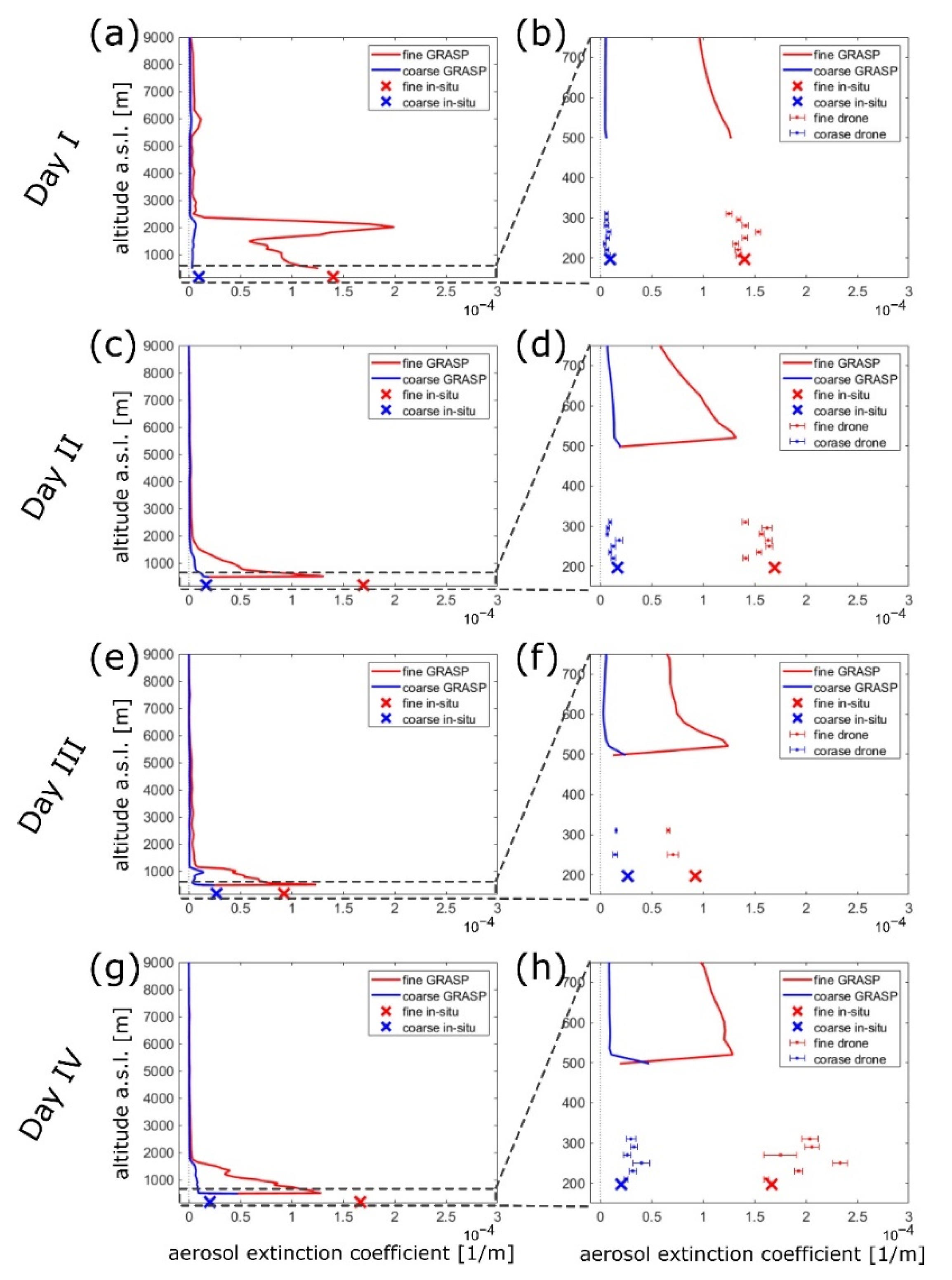
The measurement campaign, comprised of six observation days during fair weather conditions, was performed in September 2021 at the Belsk observatory. After excluding cases from two days during which a very thin layer of cirrus clouds was present (hindering credibility of high altitude retrievals with GRASP), four cases were chosen for detailed analysis, each being representative of aerosol conditions during the corresponding day.
Figure 1 shows GRASP retrievals obtained for each day in addition to extinction calculated from in-situ measurements at the ground level, and near-ground profiles from particle counters installed on UAVs.
The measurements in cases I and II were performed during low wind conditions. The calculated standard deviations of the mean values obtained from OPCs at each altitude are relatively low and allow for analysis of the distribution of aerosols within the UAV’s operation range. The wind velocities during days III and IV were much higher, up to and occasionally exceeding 5 m/s (at 2 m above ground). We observed increased battery use and overall platform instability (sudden rotations in pitch and roll axes of the drone, combined with rotor speed variability) while the UAVs struggled to maintain position over the ground against the gusts of wind. These conditions limited the available flight time while simultaneously increasing the variability of OPC measurements (possibly due to sudden changes in airspeed at the sample air intake). On day III we chose to limit the vertical resolution of the retrievals while increasing the hover times to 2 levels and 180 sec, respectively. This resulted in low standard deviations but limited the available information on the vertical structure of the aerosol layering. In contrast, during day IV we tried to perform as many 90 sec hovers as possible which resulted in six measurement points every 20 m but the standard deviations of the averaged values were much higher, on the order of magnitude of the variability between consecutive points.
In three of the studied cases, i.e., II, III, and IV, a significant mismatch between extinction at the lowermost GRASP profile point and on the ground was observed. This point represents the whole atmosphere below the profile, thus a sudden change in the value is often observed. As mentioned in
Section 2.2.3, this is a known and somewhat expected behaviour as the algorithm tries to normalize the whole α-profile to the AOD measured by the sunphotometer.
3.1. Analytical Interpolation—Closing the Extinction Profiles
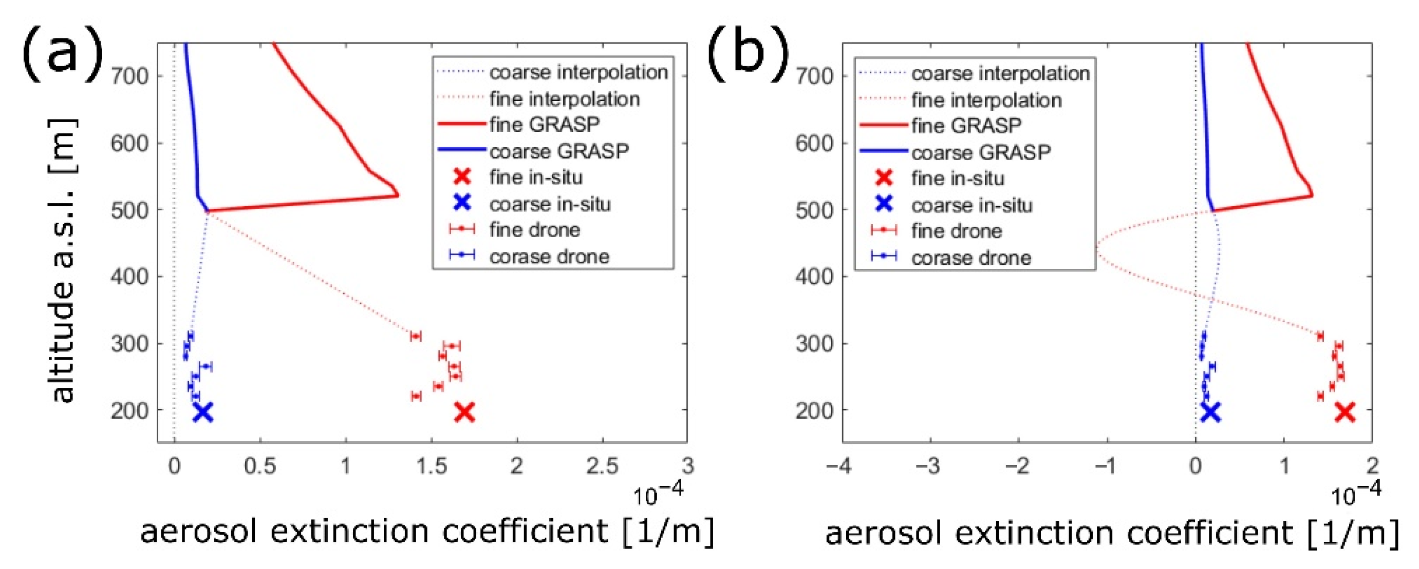
To obtain the complete profile of aerosol extinction, from the ground up to the top of the troposphere, we had to reconstruct the missing data at altitudes above the UAV operational ceiling (120 m) and below the GRASP profile (approximately 300 m above ground). The standard approach of linear interpolation has two main drawbacks. Firstly, it does not take into account rates of change (derivatives with respect to height) of the profile in regions directly neighbouring the interpolation range. This often leads to very sudden and sharp changes in the extinction values with heights that are likely not physical (see
Figure 2a). Secondly, simple linear interpolation to the values measured at or near the ground will result in the closed profile not being normalized to the columnar parameters, most importantly AOD.
To overcome the two aforementioned issues we have developed an interpolation approach based on polynomial functions. We enforce the continuity of values and first derivatives (with respect to height) at the boundaries of the interpolation region. The respective top and bottom derivatives are calculated based on the two nearest values of the GRASP and UAV profiles. This sets the total of four constraints for the interpolation function thus we use third order polynomial (defined by four free parameters) to achieve a unique solution. This method provides a smooth interpolation but is still susceptible to high variance of extinction values at the range boundaries that can often lead to unphysical negative extinction values (see
Figure 2b).
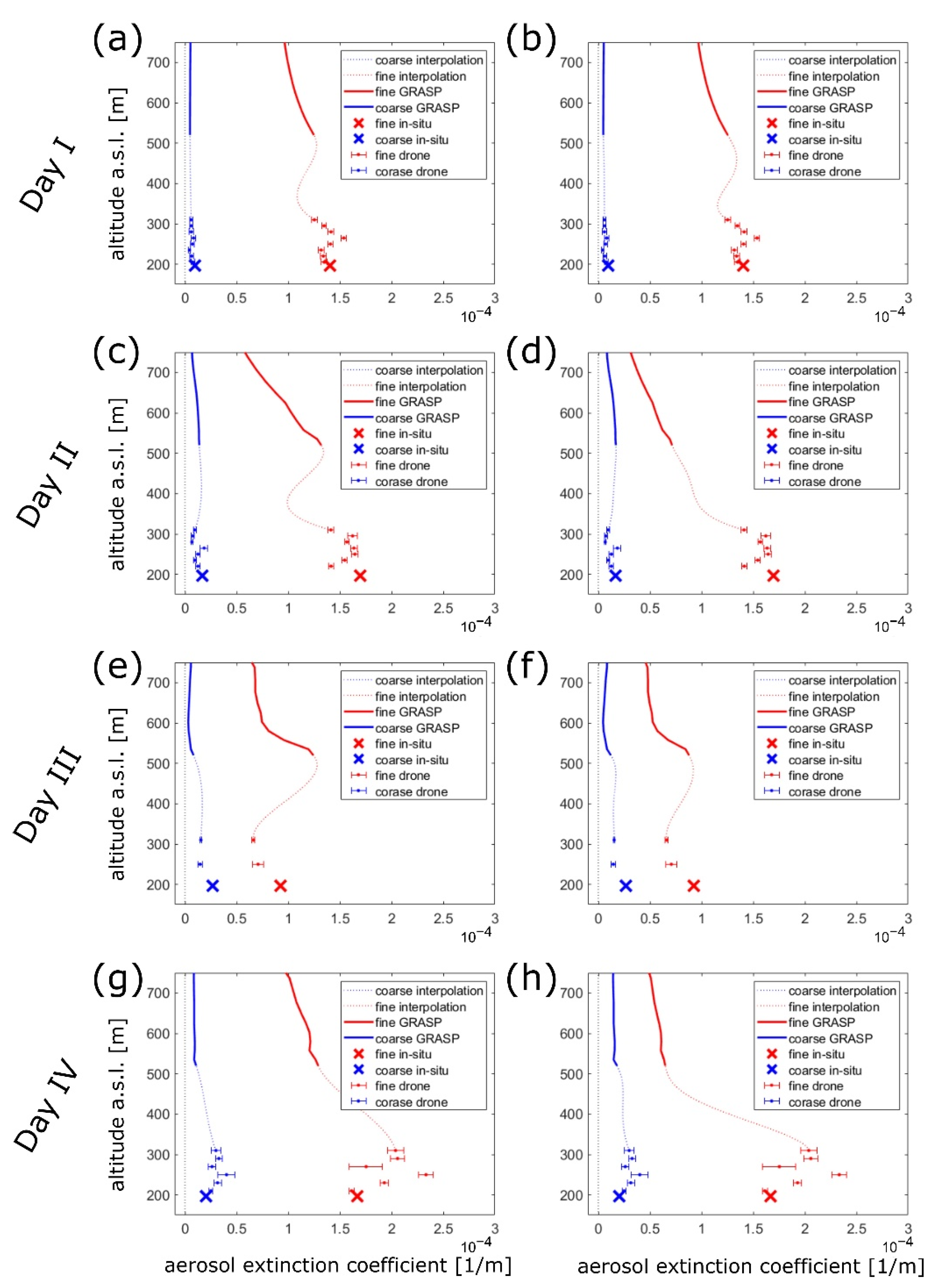
In the course of our analysis, we have formulated two possible solutions to the aforementioned issues, both of which depend on removing the lowermost value from the GRASP profile. To reiterate, this lower edge value is representative of the total content of aerosol down to the surface and is often significantly different from the values found immediately above it. It is the direct result of the algorithm’s attempt to match the extinction profile to the measured AOD. By cutting this point from the profile we can achieve much smoother interpolation at the cost of the profile no longer being normalized to the columnar optical parameters. The results of such an approach are depicted in
Figure 3 on the left-hand-side subplots.
To achieve a complete correspondence between profile and columnar values we have added additional constraints to the interpolation, namely the value of the integral of the extinction profile in the interpolation range, which can be understood as the AOD of the aerosol layer in this range. It is worth noting that optical depth is additive, thus optical depths corresponding to UAV, interpolation, and GRASP altitudes can be calculated separately (by integrating extinction) and added to obtain the total columnar AOD. This can be directly compared to the value calculated by GRASP for the LIDAR’s wavelengths based on sun-photometer observations. Such a composite approach to retrieving AOD prohibits us from excluding the lowermost GRASP value, however, as this would ensure the reconstructed profiles are no longer normalized.
We propose the following solution. Firstly, we cut the lowermost value from the GRASP profile. Secondly, we calculate partial AODs for drones and cut GRASP profiles. We subtract these two values from the total AOD to obtain the remaining AOD that should correspond to the interpolation region. Thirdly, we define five constraints: two values and two derivatives at the boundaries and an integral of the interpolated curve (equal to the layer’s AOD). Finally, we introduce an iterative approach in which we renormalize the GRASP profile and calculate corresponding interpolation functions until we arrive at a set of parameters that minimize variance (defined through standard deviation) of the interpolation curve. The results of this analysis are given on the right-hand-side subplots in
Figure 3.
3.2. Exclusion of UAV Measurements—Data Denial Experiment
To assess the advantage of utilizing UAV platforms for the reconstruction of complete extinction profiles we performed a data denial analysis where drone profile data were excluded. As there was now only a single point (at the ground) below the interpolation range the number of constraints was reduced by one (no derivative at the bottom boundary). The remaining constraints, i.e., values at both the boundaries of the interpolation range, the integral, and the derivative at the top, were used in tandem with the iterative approach to calculate the least varied (lowest standard deviation) normalized profiles. The results of such reduction in the dataset, compared with full set retrievals, are depicted in
Figure 4.
4. Discussion and Conclusions
The presented results show that the reconstruction of closed (complete) and normalized profiles of fine and coarse aerosol extinction, based on the synergy of remote, in-situ, and airborne measurement platforms, is feasible. The proposed utilization of analytical functions (in this case polynomials) coupled with the incorporation of not only values but also respective trends (derivatives with respect to altitude) at the boundaries of the interpolation region, provides smooth and stable solutions. The differences between GRASP profiles before and after the renormalization have proven to be significant (up to a factor of 1.8) in three of the investigated cases, i.e., days II, III, and IV. This is the result of a mismatch between the lowest GRASP value (representative for the lowermost part of the atmosphere, down to the surface) and the values obtained near the ground with in-situ and UAV measurements. This can be a result of prohibiting the algorithm from allocating aerosol load in the stratosphere (one of the assumptions we made in our GRASP retrievals) resulting in an overestimation of extinction in the LIDAR operational range. Such an overestimation would automatically result in an underestimation of aerosol load near the ground as the integral of the complete extinction profile is normalized to AOD. Fortunately, the method proposed in this work can overcome this problem by renormalizing the GRASP profile and thus restoring the correspondence between high and low-altitude extinction retrievals. On the day I the lowermost value in the GRASP profile was not significantly different from the neighbouring values and was similar to the values obtained near the ground, thus the renormalization did not change the profile significantly (see
Figure 3a,b).
It is worth noting that the proposed approach can in principle be utilized in a reduced form for LIDAR-derived extinction when no sunphotometric data (including AOD) is available. This is often the case when high-altitude cirrus clouds are present, creating conditions that allow for active (LIDAR) but not passive (sunphotometer) remote measurements. The comparison depicted in
Figure 3 indicates that approximate interpolation can be obtained even if the renormalization is not applied. Note however that this may lead to increased variability in the interpolation region or even produce an additional artefact layer as can be seen for day II at approximately 500 m.
The influence of wind velocity on the UAV measurements may diminish the advantage of these labour-intensive observations. Even though the manuscript presents a limited number of cases some general conclusions can be drawn nevertheless. We have found that the standard deviation of comparable drone-based OPC measurements was significantly higher on days with more windy conditions. Even though the OPC uses a small fan to drive the flow through the detector, it does not control the flow rate. It is probable that the increased motions of the UAV struggling to keep the position over the ground against the wind, combined with significant air speed in the vicinity of the aerosol inlet result in a non-constant air flow through the instrument and consequently increased measurement uncertainties.
The data denial experiment was included in this analysis to study how the additional information provided by UAV measurements enhances the overall extinction retrievals. When compared to ground-based in-situ observations alone, the utilization of airborne OPCs provides not only information on the approximate structure of aerosol extinction in the lowermost 120 m of the atmosphere but also allows for calculating a profile’s derivative at the lower boundary of the interpolation region. The results presented in
Figure 4 suggest that without drone data the extinction profiles tend to fall rapidly with height approximately within the first 100 m of the atmosphere while larger values are present higher in the GRASP profile range. The addition of UAV data results in more aerosols being represented close to the ground while the profile is renormalized to lower values in the higher troposphere. Our method exhibits slightly different behaviour in the case of day I, where the GRASP profile seems to be in better agreement with the surface values before the normalization. Although the high altitude values do not vary significantly in this case, more aerosol layers are visible thus giving additional information on the aerosol structure. In the combined regions of UAV and interpolation, there are two distinct aerosol layers visible (at approximately 250 m and 450 m) while there is rather constant aerosol extinction visible in the solution without OPC data. The results of this data denial analysis indicate that UAV data is important, if not crucial, for studying the structure of aerosol extinction near the ground, where the highest variability is often found.
To summarize, we show the profiles obtained from GRASP may be renormalized when combined with surface and near-ground measurements, in a way that preserves both smoothness of the solution and the correspondence to the columnar AOD values. Although the analysis is limited to a small number of test cases the addition of UAV-based measurements seems to enhance the quantity and quality of information on aerosol content in the vicinity of the surface. It is worth mentioning that this lowermost region of the atmosphere directly influences aerosol pollution affecting the living conditions of the human population, thus a large number of aerosol studies concentrate on this area. Such conditions are regrettably often found in the Central European industrialized regions where they pose a significant social health issue while the development of pollution mitigation strategies requires enhanced knowledge of aerosol evolution in the near-surface region of the atmosphere.
The important limitation of the presented study is the lack of independent validation of the method. This is a direct result of our efforts to incorporate all the available data into the extinction profile reconstruction scheme. Further studies are required for proper validation of the proposed approach. These may include: collocated measurements with ceilometers capable of qualitative observations of low altitude aerosol layers and thus direct comparisons with the reconstructed profiles, multi-point observations with duplicated sets of equipment allowing for direct tests of the stability of the method, and incorporation of more advanced instruments for in-situ aerosol measurements carried on larger UAVs. These ideas will be further investigated during the upcoming series of measurement campaigns.


