Prediction of Monthly PM_2.5 Concentration in Liaocheng in China Employing Artificial Neural Network

Abstract

Fine particulate matter (PM_2.5) affects climate change and human health. Therefore, the prediction of PM_2.5 level is particularly important for regulatory planning. The main objective of the study is to predict PM_2.5 concentration employing an artificial neural network (ANN). The annual change in PM_2.5 in Liaocheng from 2014 to 2021 shows a gradual decreasing trend. The air quality in Liaocheng during lockdown and after lockdown periods in 2020 was obviously improved compared with the same periods of 2019. The ANN employed in the study contains a hidden layer with 6 neurons, an input layer with 11 parameters, and an output layer. First, the ANN is used with 80% of data for training, then with 10% of data for verification. The value of correlation coefficient (R) for the training and validation data is 0.9472 and 0.9834, respectively. In the forecast period, it is demonstrated that the ANN model with Bayesian regularization (BR) algorithm (trainbr) obtained the best forecasting performance in terms of R (0.9570), mean absolute error (4.6 μg/m³), and root mean square error (6.6 μg/m³), respectively. The ANN model has produced accurate results. These results prove that the ANN is effective in monthly PM_2.5 concentration predicting due to the fact that it can identify nonlinear relationships between the input and output variables.

1. Introduction

Air pollution has a significant impact on climate change, ecosystems, and human health. Exposure to air pollution in 2019 caused 7 million premature deaths worldwide and led to the loss of millions of healthy life years [1]. In 2019, a PM_2.5 exposure level of 86% of the global urban population exceeded the world health organization (WHO) standard, resulting in 1.8 million deaths [2]. The risk of premature death attributable to PM_2.5 in China increased from 1.73 million in 2002 to 2.26 million in 2012, and then decreased slightly to 2.12 million in 2017. From 2002 to 2017, PM_2.5 in China caused an increase in deaths of more than 0.39 million. However, emission control policies and technologies prevented 0.87 million premature deaths during the same period [3]. PM_2.5 inhalation may increase the risk of premature death due to cardiovascular diseases, respiratory diseases, lung cancer, lower respiratory tract infections, brain diseases, and nervous system damage [4]. Therefore, it is necessary to accurately predict air pollution to provide people with travel patterns.

Artificial intelligence (AI) is widely used in air pollution prediction [5]. The Backwards Propagation (BP) neural network algorithm is used to predict the quality of PM_2.5 in Chongqing, which indicates that it is feasible to use a neural network to predict air quality [6]. The artificial neural network (ANN) is used to forecast PM_2.5 concentration with 80% of data for training then with 90% of data for training in Ahvaz. The value of R for the data validation of these two networks was 0.80 and 0.83, respectively [7]. A backpropagation artificial neural network (BPANN) combined with an adaptive multi-objective particle swarm optimizer (AMOPSO) algorithm based on computational fluid dynamics (CFD) is used to predict indoor PM_2.5 concentrations. The proposed optimization algorithm reduces PM_2.5 concentrations by as much as 77.1% [8]. Four modeling techniques, including time-integrated activity, Monte Carlo simulation, ANN, and principal component analysis (PCA), are utilized to predict exposure values of PM_2.5. The results of a time-weighted activity model display the lowest correlation with measured values. For Monte Carlo simulation, high correlation is obtained. Compared with the simple ANN models, the PCA-ANN exports the most accurate results [9]. To summarize, numerous studies show that ANN can be used to define functional relationships between dependent and independent variables.

Deep learning displays prodigious potential in fitting nonlinear complex relationships between the influencing factors and the pollution concentrations [10], and includes the convolutional neural network (CNN) [11] and recurrent neural network (RNN) [12]. A convolutional neural network (CNN) can learn the characteristics of data by directly inputting the original image, which has been widely used in recent years. A deep learning-based response surface model (deepRSM) is established based on the deep learning method, which uses artificial intelligence to achieve more accurate response surface fitting, solves the problem of rapid prediction of pollution control effects, and significantly improves the applicability and effectiveness of the response surface model (RSM) for decision-making assistance [10]. The CNN model on the air quality dataset is utilized to detect patterns for future prediction modeling in India [11]. Nonetheless, the accuracy of the CNN model is measured to determine the applicability of algorithm. The multi-directional temporal convolutional artificial neural network (MTCAN) model maintains the temporal correlation within the features’ measurement and meteorological and pollutant variables to impute and forecast PM_2.5 missing values [13]. A novel machine learning-based model (MCNN-BP) is proposed by multiple convolutional neural networks (MCNN) and backpropagation neural networks for making spatiotemporal PM_2.5 prediction at 74 stations in Taiwan [14].

A long short-term memory (LSTM) neural network is a RNN with long-term and short-term memory. The LSTM approach is also used for predicting O₃, PM_2.5, NO_x, and CO concentrations at a location in NCT-Delhi [15]. Geo-LSTM for predicting PM_2.5 has an RMSE of 0.0437, and performs almost 60.13% better than IDW [16]. The LSTM model outperformed random forest (RF) and Cubist approaches for predicting PM_2.5 because of its RNN structure that can capture time dependence and nonlinear relationships among PM_2.5 concentrations and other independent variables, and exhibited a stable accuracy with an R² of 0.83 [17]. A workflow of future PM_2.5 concentrations prediction was developed based on an LSTM model. Using ground-based station PM_2.5 data in 2014–2018, the 1 km MAIAC AOD product and other auxiliary data were used to predict PM_2.5 concentrations in the next year and generate a national PM_2.5 spatial map in China [17]. A novel hybrid prediction model was constructed by combining the empirical mode decomposition (EMD), sample entropy (SE), and bidirectional long- and short-term memory neural network (LSTM) to predict PM_2.5 concentrations [18]. A new PM_2.5 prediction method based on a hybrid model of complete ensemble empirical mode decomposition with adaptive noise (CEEMDAN) and bi-directional long short-term memory (BiLSTM) is presented. The CEEMDAN-FE can effectively reduce the instability and high volatility of the original PM_2.5 data, overcome data noise, and prominently enhance the model’s performance in forecasting PM_2.5 concentration [19]. The CNN-LSTM model is also proposed to predict air quality, and both the CNN-LSTM and the LSTM generally have better performance than the CNN and the BPNN [20]. The advanced deep predictive convolutional LSTM (ConvLSTM) model paired with the cutting-edge graph convolutional network (GCN) architecture is used to predict hourly PM_2.5 in the Los Angeles area. The RMSE and NRMSE of the model show significant improvement over existing research in predicting PM_2.5 concentration [21]. Although the deep learning model can improve the prediction ability to some extent, it requires massive data for training, and it has its scope of application, which leads to different prediction performance of PM_2.5 concentration time series in different ranges.

The sudden outbreak of COVID-19 has not only seriously impacted global economic activities, but also profoundly affected people’s living patterns [22]. Up to 30 June 2022 globally, over 6,332,963 people have died, and 544,324,069 have been infected with COVID-19 (WHO). In response to the epidemic, large measures such as shutdown and home isolation have been taken all over the world, with unprecedented intensity and duration, which provides a unique natural experimental condition for exploring the potential of global air pollution reduction. This scenario provides an opportunity to understand and study air pollution control and emission reduction measures. During COVID-19, the NO concentrations decreased by 58–70% in two towns in Paraiba Valley: São José dos Campos and Guaratinguetá, Brazil [23]. PM_2.5, NO₂, and CO were reduced during COVID-19 in 2020 in Chicago, IL, USA [24]. Brazil’s air quality improved due to mobility restrictions imposed by COVID-19 [25]. After the lockdown, the PM_2.5 pollution load throughout the whole area in Lodz, Poland, and across its central parts in particular, decreased dramatically [26]. Car transportation was limited due to the COVID-19 lockdown in Poland. Car transportation in Krakow is responsible for up to 20% of the PM₁₀ carbon fraction concentration [27]. During the lockdown period, CO, NO, NO₂, SO₂, and PM_2.5 decreased by 64%, 1.5%, 75%, 24%, and 54%, respectively, compared to concentrations of these pollutants in 2019 in Bishkek, Kyrgyz Republic [28]. NO_x emission in China in the lockdown period was 53.4% lower than the same period in 2019 [29]. The concentrations of atmospheric components in many countries and regions have also experienced a process of sharp decline, low-level maintenance, and slow recovery. Air pollution mainly comes from traffic, industry, and power plant emissions. Therefore, the change in air pollution can well reflect the change in social and economic activities during the epidemic. By studying the air pollution observation data, the spatial and temporal change pattern of air pollution during the COVID-19 epidemic was revealed [29].

Many artificial intelligence techniques have been utilized to forecast PM_2.5 concentration. Nevertheless, there are many challenges for precise prediction by diverse methods. It is very difficult to cultivate precise artificial intelligence techniques with small PM_2.5 datasets. Deep learning methods are successful owing to big training data which can be used to predict PM_2.5 concentration. It is difficult to pitch appropriate architectures and parameters for deep learning methods with small PM_2.5 datasets.

An artificial neural network (ANN) has the advantage of processing small data. Therefore, we use an ANN to predict the monthly air pollution in Liaocheng City. Liaocheng is a typical air pollution city in northern China. In this article, PM_2.5 in Liaocheng in Shandong Province, China, from 2014 to 2022 was investigated. Moreover, seasonal and annual changes in PM_2.5 concentration have been analyzed in this study. If the PM_2.5 time series to be modeled is sufficiently auto-correlated, the time series prediction model is developed using an artificial neural network, and then the performance of the different algorithms is tested. For different combinations of input variables, the different parameters are compared, including input variables, hidden layer neurons, and transfer functions. We also calculate the periodicity of the PM_2.5 time series and evaluate the generalization ability and the parameter uncertainty of the model development model. Overall, despite the limited PM_2.5 data used in this study, the developed ANN model is capable of predicting monthly PM_2.5 concentration over the study area reasonably well.

The remainder of this paper is as follows. Section 2 is devoted to artificial neural network and air pollution data in Liaocheng. In Section 3, we analyze long-term changes in the air quality in Liaocheng, predict the PM_2.5 concentration in Liaocheng, and compare with existing models. We discuss the topologies of the ANN. In Section 4, we summarize the paper and put forward the future prospects of air pollution prediction.

2. Materials and Methods

Liaocheng City is located in the west of Shandong Province in China (Figure 1), facing Handan City and Xingtai City in Hebei Province across the Zhangwei River in the west, and adjacent to Tai’an City and Jinan City and Henan Province across the Jindi River and the Yellow River in the south and southeast. Liaocheng is on a Yellow River alluvial plain, high in the southwest and low in the northeast, with an altitude of 22.6–49.0 m. Liaocheng covers a total area of 8628 square kilometers. By the end of 2021, Liaocheng had a permanent population of 5.9279 million. In 2021, Liaocheng achieved a regional GDP of CNY 264.252 billion. It has a semi-arid continental climate. The annual average temperature of Liaocheng City is 13.5 °C, the average temperature of January is −1.8 °C, and the average temperature of July is 26.8 °C. The annual average precipitation is 540.4 mm, and the annual mean wind speed is 2.3 m/s.

As shown in

Table 1. Chinese ambient air quality standards.

Air Pollutants	Index	Grade I Value	Grade II Value
PM2.5 (μg/m3)	Annual average	15	35
	24 h average	35	75
PM10 (μg/m3)	Annual average	40	70
	24 h average	50	150
O3 (μg/m3)	Maximum of daily 8 h moving average	100	160
NO2 (μg/m3)	Annual average	40	40
	24 h average	80	80
SO2 (μg/m3)	Annual average	20	60
	24 h average	50	150
CO (mg/m3)	24 h average	4	4

, the most recent Chinese ambient air quality standards (CAAQS) (GB3095-2012) were published in 2012, when PM_2.5 and O₃-8h were added for the first time [30]. In 2012, a ‘Technical Regulation on Ambient Air Quality Index’ (HJ 633-2012) released by the Chinese Ministry of Ecology and Environment (MEE) (https://www.mee.gov.cn/, accessed on 1 January 2021) replaced the air pollution index (API) with AQI and divided air quality into six levels (

Table 2. AQI scope and air quality category.

AQI Value	Level	Category	Color Indication
0–50	I	Excellent	Green
51–100	II	Good	Yellow
101–150	III	Mild pollution	Orange
151–200	IV	Moderate pollution	Red
201–300	V	Heavy pollution	Purple
>300	VI	Serious pollution	Maroon

) [30].

CO is measured utilizing the non-dispersive infrared absorption method, PM_2.5 and PM₁₀ are measured utilizing the micro-oscillating balance method and the β absorption method, and SO₂, NO₂, and O₃ are measured by the fluorescence method, the chemiluminescence method, and the UV-spectrophotometry method, respectively [31].

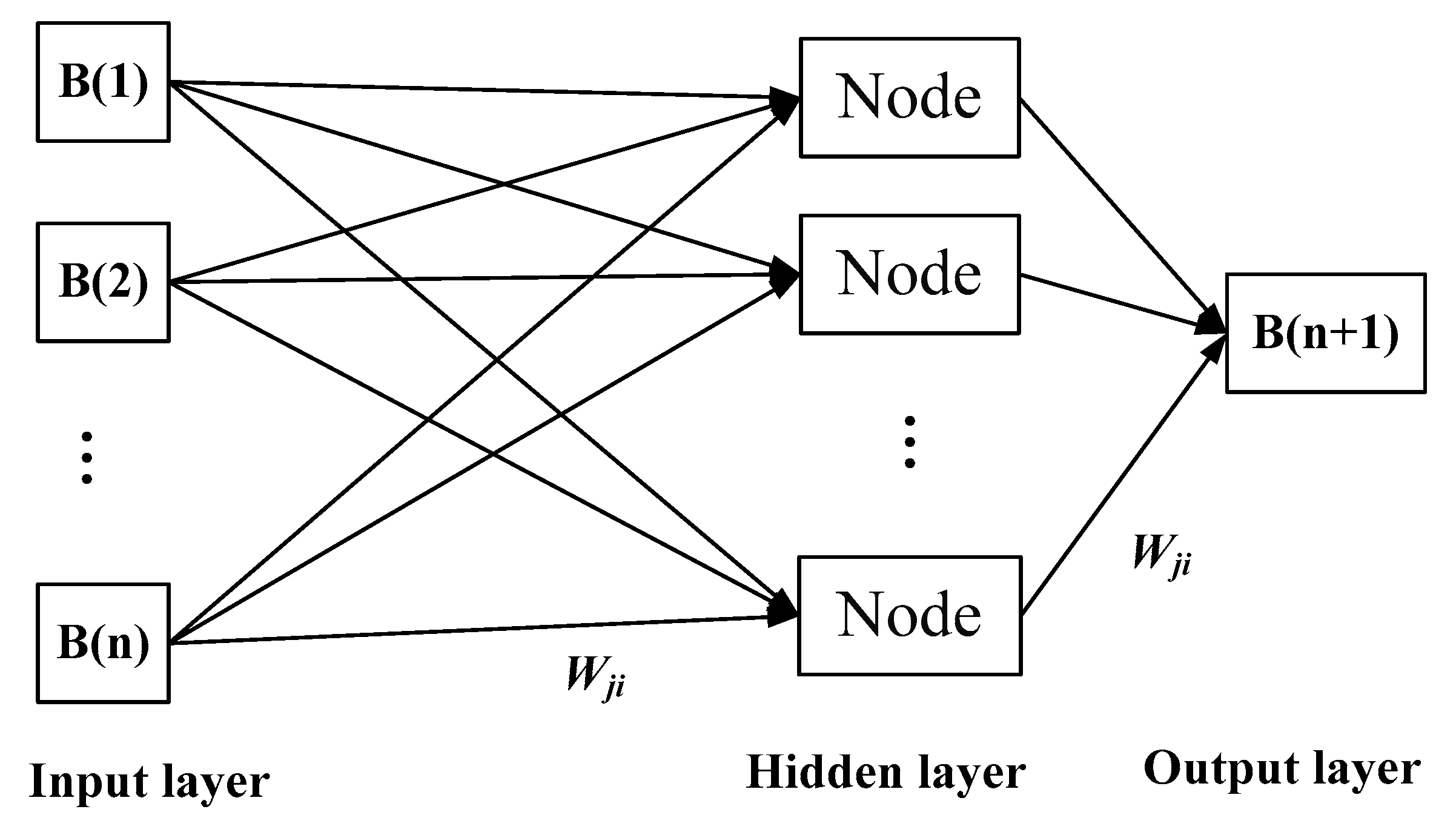
Backpropagation artificial neural network (BPANN) model topology includes an input layer, an output layer, and a hidden layer. Each layer for BPANN has a particular number of nodes depending on the complexity of the question. Each node in the input and hidden layer is connected to each of the nodes in the coming layer (hidden or output) by a weight factor and a bias value. The BPANN is a training algorithm and its learning rule is to utilize the steepest descent method to continuously adjust the weights and bias of the neural network by utilizing the backpropagation of the error [32]. To avoid overfitting and to validate the stability of the ANN model, we use 80% of the data for training and 10% of the data for examining. B(1)…B(n) are the data of monthly PM_2.5 concentration as the input variable, and B(n + 1) is PM_2.5 predicted for +1 month (Figure 2). B_i is the node input, s expresses the node output, and W_ji expresses the weight, where P expresses the node excitation threshold, and a and t express the basic and activation functions, respectively. A node assesses the weighted summation of the inputs as:

$$\mathrm{a}=(W_{ji}{B}_i)+P$$

(1)

The activation function appraises output by:

$$\mathrm{s}=\mathrm{t}(\mathrm{a})$$

(2)

The properties of the ANN model are appraised using three norms containing: correlation coefficient (R), root mean square error (RMSE), and mean absolute error (MAE). The R values are used to determine the model precision, and the RMSE values are used to determine the residuals between predictions and actual PM_2.5 values [33].

$$RMSE=\sqrt{\frac{{\displaystyle \sum {(F_k-H_k)}^2}}{Q}}$$

(3)

$$R=\frac{{\displaystyle \sum (F_k-\stackrel{-}{F})(H_k-\stackrel{-}{H})}}{\sqrt{{\displaystyle \sum {(F_k-\stackrel{-}{F})}^2{(H_k-\stackrel{-}{H})}^2}}}$$

(4)

$$MAE=\frac{1}{Q}{\displaystyle \sum \left|F_k-H_k\right|}$$

(5)

$F_k$ denotes the actual PM_2.5 concentration, $H_k$ denotes the predicted PM_2.5 concentration, $\stackrel{-}{F}$ is the mean of the actual PM_2.5 concentration, and $\stackrel{-}{H}$ is the mean of the predicted PM_2.5 concentration.

The software we use is matlabR2010a, which was created by Little J. and Moler C., and it is from MathWorks Inc, Natick, MA, USA [34]. The values of air quality index (AQI), PM₁₀, PM_2.5, NO₂, SO₂, CO, and O₃ in Liaocheng from January 2014 to May 2022 are investigated (http://www.aqistudy.cn/, accessed on 1 June 2022), and these data are divided into three parts: training period (January 2014 to September 2020); verification period (October 2020 to July 2021); prediction period (August 2021 to May 2022) (Figure 3).

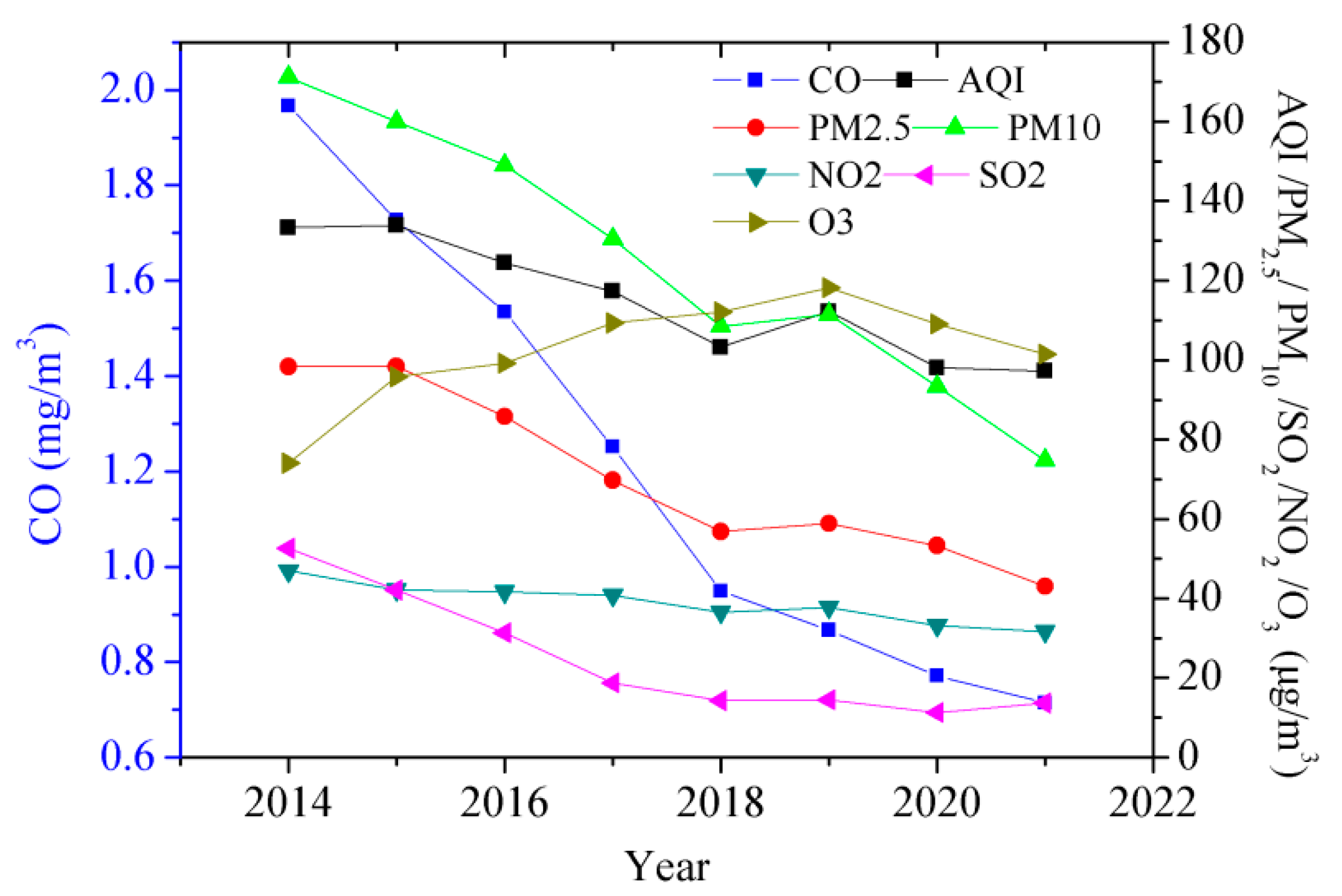
The average concentrations of the air pollutants during 2014–2021 in Liaocheng are analyzed. SO₂ (2014–2021) and NO₂ (2019–2021) concentrations in Liaocheng meet the national Grade I or Grade II for annual mean ambient air quality. NO₂ (2014–2018), PM_2.5 (2014–2021), and PM₁₀ (2014–2021) concentrations in Liaocheng exceed the national Grade II for annual mean ambient air quality. AQI values (2020–2021) meet national Level II, but AQI values (2014–2019) exceed national Level II.

3. Results and Discussion

In this section, we analyze the research results and discuss the structure of the artificial neural network. Firstly, the air quality in Liaocheng from 2014 to 2021 is analyzed, and the effects of the almost complete lockdown on air quality are analyzed. Finally, PM_2.5 concentrations from January 2014 to May 2022, are simulated and predicted using the artificial neural network.

3.1. Long-Term Changes in the Air Quality in Liaocheng

As shown in Figure 3, the air quality in Liaocheng gradually improved year by year. The formula for calculating the reduction rate of air quality is as follows:

$$D=\frac{\left(A_{\mathrm{i}}-A_{\mathrm{j}}\right)}{A_{\mathrm{i}}}\times 100\%$$

(6)

D is the reduction rate of air quality, and A_i and A_j are air quality.

Therefore, the reduction rates of AQI, PM_2.5, PM₁₀, SO₂, CO, NO₂, and O₃ from 2014 to 2021 in Liaocheng were 27.1%, 56.2%, 56.3%, 74.0%, 63.7%, 32.5%, and −37.2%, respectively. Air quality in 2021 was sharply better than that in 2014. However, the concentration of O₃ increased by 37.2%, and its change trend was different from that of other pollutants. Although the concentration of PM_2.5 in Liaocheng has decreased significantly in recent years, there is still a big gap from the World Health Organization guidelines, and the ozone problem is becoming increasingly prominent. Clean air policies play an important role in reducing air pollution, and these policies include the action plan for the prevention and control of air pollution, the three-year action plan for the defense of the blue sky, the program for tackling key problems of air pollution in autumn and winter in key areas, and the “one city, one policy” for coordinated prevention and control of fine particulate matter and ozone pollution.

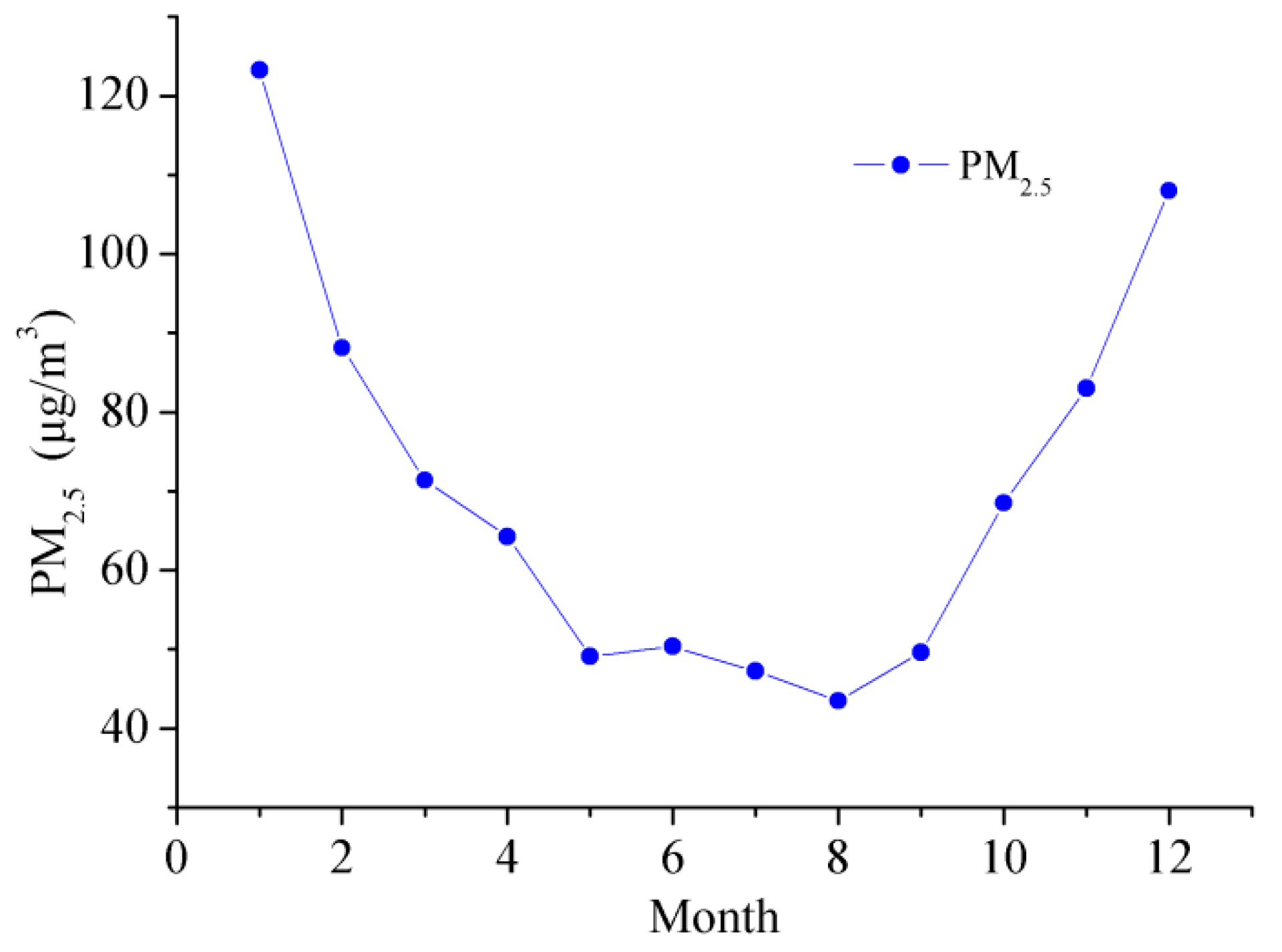
The concentration of PM_2.5 in Liaocheng from 2014 to 2021 has obvious seasonal variation characteristics. The average concentration of PM_2.5 in spring, summer, autumn, and winter was 61.6, 47.0, 67.0, and 106.5 (μg/m³), respectively. The seasonal average concentration of PM_2.5 in Liaocheng is the lowest in summer and the highest in winter. The variation trend of the average concentration of PM_2.5 in Liaocheng over four seasons is: summer < autumn < spring < winter.

As shown in Figure 4, the monthly average concentration of PM_2.5 in Liaocheng from 2014 to 2021 also has obvious characteristics of monthly variation, and the average concentration of PM_2.5 shows a “U” shape. For example, the concentration of PM_2.5 in January is calculated by calculating PM_2.5 concentration in January from January 2014 to January 2021. The average concentration of PM_2.5 was the highest in January and the lowest in August.

3.2. Air Quality Changes before, during, and after the Lockdown Period

These data are divided into three parts: period I (before the lockdown) (1 January to 26 January 2019 and 2020); period II (during the lockdown) (27 January to 30 April 2020); period III (after the lockdown) (1 May to 20 July 2020). First, we make statistical analysis for air quality in Liaocheng, from 1 January to 20 July in 2020, and these results are shown in Figure 5. The reduction rates of AQI, PM_2.5, PM₁₀, SO₂, CO, NO₂, and O₃ from period I to period II in Liaocheng were 53.9%, 64.1%, 51.1%, 26.0%, 61.6%, 52.7%, and −106.4%, respectively. Those from period II to period III in Liaocheng were, respectively, 21.9%, −30.3%, −11.3%, −6.2%, −8.5%, −12.8%, and 52.1%. These results indicate that the air quality during lockdown was obviously improved compared with before and after lockdown periods.

In the same period (before lockdown) of 2019, the average values of AQI, PM_2.5, PM₁₀, SO₂, CO, NO₂, and O₃ were, respectively, 150.2, 112.1, 183.6, 25.6, 1.42, 63.4, and 49.8 (μg/m³ (CO (mg/m³))), which was a decline of 20.4%, 24.3%, −3.0%, −44.7%, 20.9%, − 11.1%, and 0.2%, compared with that of before lockdown 2020. However, in the same period (during lockdown) of 2019, those were, respectively, 110.7, 74.0, 134.8, 15.4, 0.89, 36.7, 106.3 (μg/m³ (CO (mg/m³))), which is a decline of −24.7%, −32.3%, −35.4%, −32.2%, −25.8%, −27.5%, and −3.2%, compared with that of during lockdown in 2020. Those were, respectively, 124.6, 35.1, 86.9, 14.7, 0.65, 26.4, and 184.6 (μg/m³ (CO (mg/m³))) in the same period (after lockdown) of 2019, which is a decline of −18.5%, −0.6%, −11.0%, −32.9%, −6.9%, −11.9%, and −15.2% compared with that of after lockdown in 2020. It is also worth noting that all the changes in air pollution during the lockdown period and after lockdown (2019–2020) are consistent. These results also indicate that the air quality in Liaocheng during lockdown and after lockdown periods in 2020 was obviously improved compared with the same periods of 2019. However, air quality in Liaocheng before lockdown in 2020 was worse than that of the same period of 2019.

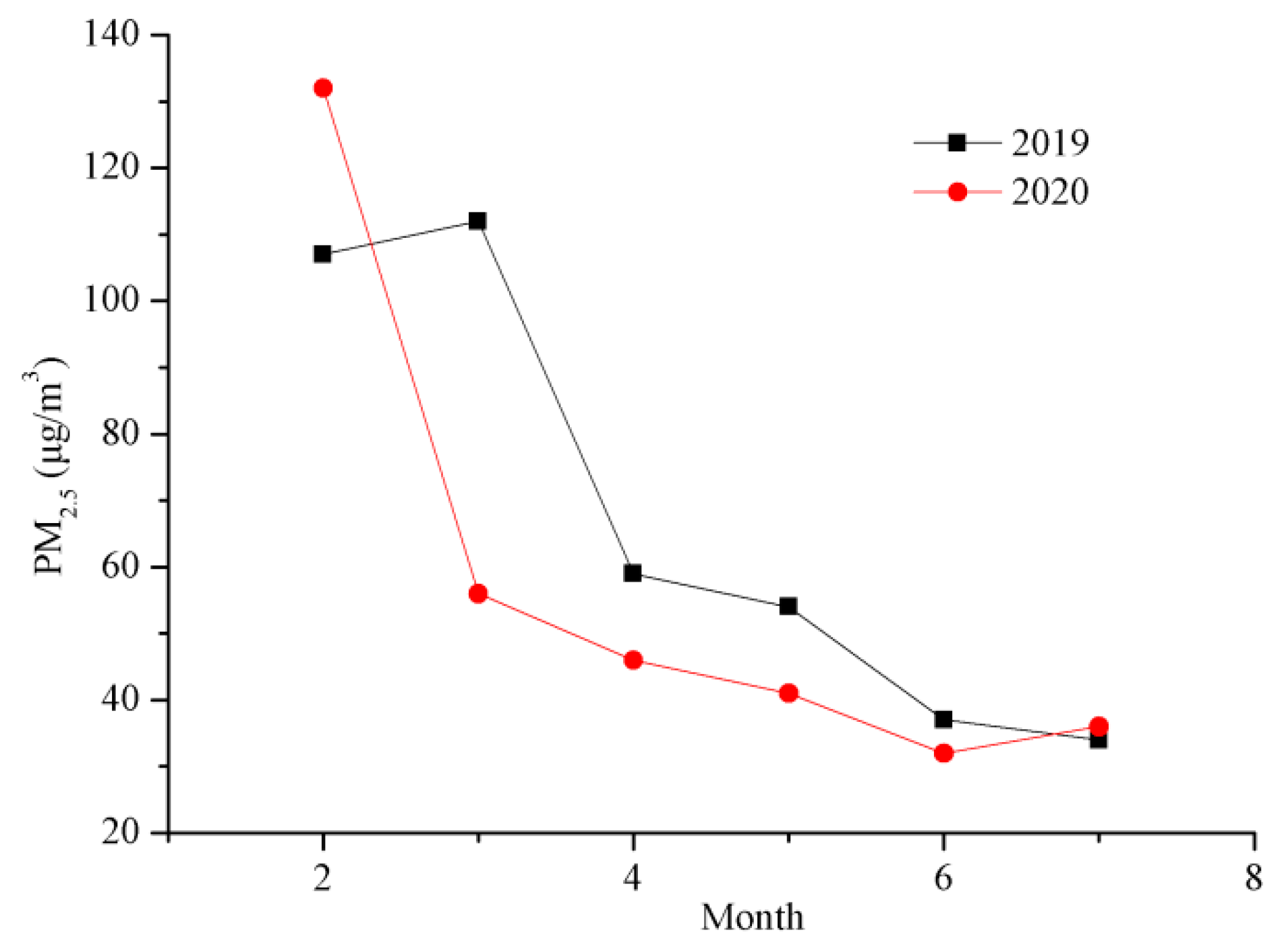
As shown in Figure 6, in Liaocheng during January–June 2019, the monthly average PM_2.5 concentrations were 107, 112, 59, 54, 37, and 34 (μg/m³), respectively, while those during January–June 2020 were 132, 56, 46, 41, 32, and 36 (μg/m³), respectively, which were 23.4%, −50.0%, −22.0%, −24.1%, −13.5%, and 5.9% higher than those during January–June 2019, respectively.

3.3. Model Design Employing the Artificial Neural Network Modal

The cycles of monthly PM_2.5 concentration in Liaocheng were calculated using wavelet analysis (Figure 7). The wavelet variance can reflect the distribution of wave energy of a time series. It can be used to determine the main periods of monthly PM_2.5 concentration. There are three obvious peaks in the wavelet variance chart, which correspond to the time scales of 10 months, 21 months, and 33 months (Figure 7). These are the cycles of monthly PM_2.5 concentration. Among them, the maximum peak value corresponds to the 10 months, which means that the period oscillation of about 10 months is the strongest, and it is the first main cycle; the second peak corresponds to the 21 months, which is the second main cycle; the third peak value corresponds to 33 months. This shows that the fluctuation of the above three periods controls the variation characteristics of monthly PM_2.5 concentration in Liaocheng.

The numbers of nodes in input and hidden layers are tested by trial and error. The performance of different numbers of nodes in the input layer (

Table 3. Comparison of R, RMSE(μg/m³), and MAE (μg/m³) between various input variables.

Variables	R			RMSE			MAE
	Training	Verification	Predicting	Training	Verification	Predicting	Training	Verification	Predicting
1	0.7681	0.6441	0.521	21.3	16.2	20.1	15.8	14.1	14.8
2	0.7929	0.7042	0.5354	20.2	15.4	21.2	14.3	12.5	14.3
3	0.7966	0.7985	0.6318	20.1	13.5	20.0	14.3	10.9	13.8
4	0.7995	0.7693	0.6797	20.0	15.0	19.9	14.2	12.5	13.8
5	0.8408	0.8678	0.6332	18.5	12.8	18.6	12.9	10.7	13.5
6	0.8627	0.8635	0.8844	17.3	12.1	12.7	12.0	9.8	10.4
7	0.8115	0.8815	0.8571	22.7	16.7	15.4	14.1	14.9	12.7
8	0.8166	0.8962	0.8651	21.1	19.2	18.3	14.2	16.9	15.7
9	0.7395	0.786	0.7721	29.3	15.2	14.8	18.2	13.3	11.2
10	0.8612	0.8433	0.8146	19.0	12.5	13.2	12.1	10.6	10.4
11	0.9472	0.9834	0.957	10.9	4.4	6.6	7.7	3.5	4.6
12	0.9055	0.9716	0.8691	14.4	7.3	11.1	9.3	5.8	9.5
13	0.9012	0.9709	0.8725	15.5	5.7	11.0	9.2	4.5	9.3
14	0.8534	0.7204	0.8474	19.9	15.5	16.8	12.0	12.0	13.0
15	0.839	0.9314	0.8224	20.7	11.8	20.3	12.5	9.3	16.4
16	0.8632	0.8927	0.849	19.6	11.9	17.7	11.5	8.0	14.1

) and hidden layer (

Table 4. Comparison of R, RMSE(μg/m³), and MAE (μg/m³) between different nodes in the hidden layer.

Nodes	R			RMSE			MAE
	Training	Verification	Predicting	Training	Verification	Predicting	Training	Verification	Predicting
1	0.9036	0.9202	0.692	14.5	8.6	15.4	10.2	7.6	12.3
2	0.904	0.9214	0.6925	14.4	8.6	15.4	10.1	7.6	12.3
3	0.9209	0.9478	0.811	13.1	7.5	12.6	8.7	5.9	9.4
4	0.9256	0.9351	0.8176	12.8	9.4	12.5	8.8	7.8	9.0
5	0.9167	0.9537	0.9106	14.2	8.3	9.1	9.6	7.3	7.4
6	0.9472	0.9834	0.957	10.9	4.4	6.6	7.7	3.5	4.6
7	0.8387	0.9573	0.7978	22.5	13.9	19.8	14.8	13.2	16.9
8	0.7771	0.8386	0.782	27.6	12.0	15.9	18.3	9.3	13.6
9	0.8252	0.8355	0.8441	23.4	19.5	19.4	16.1	17.1	16.9
10	0.8621	0.8802	0.844	21.8	15.7	19.3	14.2	13.3	17.3
11	0.7772	0.8657	0.7922	29.8	14.2	15.5	19.5	12.8	12.8
12	0.8136	0.8148	0.8137	28.5	15.2	15.5	18.6	13.6	12.9
13	0.7768	0.8949	0.712	27.9	13.2	17.7	18.0	12.4	14.2
14	0.8399	0.9616	0.8523	24.6	14.8	18.5	16.6	14.1	17.1
15	0.7105	0.8186	0.7954	33.1	14.0	16.6	21.7	11.4	13.0
16	0.8028	0.8966	0.8283	28.5	11.5	16.1	19.2	10.5	14.2

) is contrasted. Table 3 indicates the various input variables and Table 4 indicates different nodes in the hidden layer. Table 3 and Table 4 show simulation of PM_2.5 during the training, verification, and predicting periods. Eleven variables were selected for the model input. We used the most recent 11 months from September 2020 to July 2021 during the predicting period. Furthermore, the number of neurons of the hidden layer was similarly six. Finally, network topologies of the ANN (11-6-1) were the best.

Training algorithms of the ANN are also selected by trial and error.

Table 5. Comparison of R, RMSE(μg/m³), and MAE (μg/m³) between various training algorithms.

Training Functions	R			RMSE			MAE
	Training	Verification	Predicting	Training	Verification	Predicting	Training	Verification	Predicting
trainbr	0.9472	0.9834	0.9570	10.9	4.4	6.6	7.7	3.5	4.6
trainlm	0.9158	0.9094	0.6952	13.5	9.3	15.3	9.3	6.9	11.8
traingdx	0.7385	0.7806	0.6020	23.3	23.2	25.4	18.0	19.6	21.4
traingd	0.6446	0.8103	0.7158	26.4	21.5	27.0	18.8	17.1	22.5
traingdm	0.6469	0.8017	0.6042	26.1	19.0	25.6	19.6	15.0	19.7
trainrp	0.4024	0.4660	0.6717	31.1	22.4	25.5	23.4	18.3	20.9
traincgp	0.8072	0.7114	0.7576	20.5	21.6	24.6	14.6	16.0	19.7
traincgf	0.7026	0.7686	0.4458	24.4	18.6	28.8	18.9	16.5	25.3
traincgb	0.6722	0.5321	0.7767	25.6	28.8	22.3	19.0	24.7	17.7
trainscg	0.8615	0.9518	0.8442	20.0	12.4	14.6	11.7	10.8	11.2
trainbfg	0.6573	0.8805	0.7233	26.0	17.3	28.7	19.8	14.5	24.3
trainoss	0.6198	0.6442	0.7081	26.8	22.4	24.3	20.6	18.4	21.3

indicates the performances of training algorithms for forecasting PM_2.5 concentration. Trainbr is an algorithm of Bayesian regularization (BR) backpropagation, and it is a network training function that updates weights and deviation values on the basis of Levenberg Marquardt optimization. It minimizes the combination of squared errors and weight values, and then defines the correct combination to generate a network with good generalization. Trainbr is the algorithm that best predicted the PM_2.5 concentration. It showed the best performance in simulating PM_2.5 during the training period, the verification period, and the prediction period. The simulated PM_2.5 concentration was very close to the actual PM_2.5 concentration. To avoid overfitting problems, a test experiment wad conducted. The ANN model has analogous R values, so consequently there were no overfitting problems with the ANN model. The RMSE value for the ANN employing trainbr for the training period is 10.9 μg/m³, and that for the verification period is 4.4 μg/m³. The R values for the ANN employing trainbr during the training and verification periods were 0.9472 and 0.9834, respectively. The MAE for the ANN using trainbr were 7.7 μg/m³ and 3.5 μg/m³, respectively.

Transfer functions of the ANN are picked by trial and error.

Table 6. Comparison of R, RMSE(μg/m³), and MAE (μg/m³) between various transfer functions.

Transfer Function	R			RMSE			MAE
	Training	Verification	Predicting	Training	Verification	Predicting	Training	Verification	Predicting
tansig-purelin	0.8240	0.8996	0.7771	22.7	13.0	20.0	13.9	10.0	16.2
tansig-logsig	0.7326	0.8685	0.7129	31.0	12.6	16.1	20.2	10.7	11.9
tansig-tansig	0.7431	0.8821	0.7247	30.5	11.3	15.2	19.6	9.3	11.0
logsig-purelin	0.8343	0.9089	0.8501	22.9	11.5	16.4	14.2	9.6	14.9
logsig-tansig	0.6720	0.7507	0.5837	36.9	15.4	18.1	25.0	11.9	13.7
logsig-logsig	0.8166	0.9096	0.8943	24.2	12.7	13.2	15.2	10.6	11.1
purelin-tansig	0.6712	0.7809	0.6515	37.3	16.3	18.4	25.7	13.1	14.7
purelin-logsig	0.9042	0.9219	0.6969	14.4	8.6	15.3	10.1	7.5	12.1
purelin-purelin	0.8980	0.9741	0.7115	14.8	5.2	15.2	10.3	4.4	12.2
tansig-poslin	0.8664	0.9645	0.9338	21.5	5.2	7.8	12.1	4.5	6.1
logsig-poslin	0.9472	0.9834	0.9570	10.9	4.4	6.6	7.7	3.5	4.6
poslin-poslin	0.8980	0.9741	0.7115	14.8	5.2	15.2	10.4	4.5	12.2
purelin-poslin	0.8936	0.9784	0.7210	25.9	12.7	20.3	19.8	11.2	14.9

indicates that the transfer function logsig-poslin is better than others during training, verification, and predicting stages. Purelin is a linear transfer function and poslin is a positive linear transfer function. Tansig is a hyperbolic tangent sigmoid transfer function and logsig is a logarithmic sigmoid transfer function.

3.4. Prediction of the PM_2.5 Concentration in Liaocheng and Comparison with Existing Models

In the forecast period, PM_2.5 concentration in the next month is predicted employing the previous months’ PM_2.5 concentration. Table 6 indicates the predicting performance employing trainbr for the designed ANN model. For PM_2.5 concentration in Liaocheng during the predicting period, the R, RMSE, and MAE are 0.9570, 6.6 μg/m³, 4.6 μg/m³, respectively.

Figure 8 makes clear predicted PM_2.5 concentration. The training and verification values are from January 2014 to July 2021. Then, we began to predict from August 2021 to May 2022. In both the training stage and the verification stage, the simulated values and the observed values are very close, especially in the simulated minimum value. In the 10 months, the forecasting PM_2.5 concentration is similar to the actual PM_2.5 concentration.

Different models for predicting PM_2.5 concentration are evaluated in

Table 7. The difference between existing PM_2.5 models and the proposed ANN model.

Literature	Model	Area	R2	RMSE (μg/m3)	MAE (μg/m3)
[7]	ANN	Ahvaz, Iran	0.74
[35]	BRNN/FFS	Kaohsiung, Taiwan, China	0.95	2.7381	2.3292
[36]	MLP	Eastern China, China		41.97	31.11
[37]	Aggregated LSTM	Taiwan, China		3.94	2.94
[38]	LSTM	Kathmandu valley, Nepal		13.04	10.81
[39]	WBBNN	Beijing, China	0.8371	33.812	34.515
[40]	BPNN	Beijing, China		24.06
[41]	ANN	Delhi, India	0.86
[42]	ANN	Addis Ababa, Ethiopia	0.943
[43]	LSTME	Beijing, China		12.6	5.46
[44]	CNN-LSTM	Beijing, China	0.921573	24.22874	14.63446
[45]	CNN	United States	0.84	2.55	1.56
[46]	3D CNN-GRU	The great Tehran	0.78	6.44	8.89
[47]	CEEMDAN-DeepTCN	Beijing, China		1.1064	0.6561
[48]	CNN-GBM	Shanghai, China	0.85	10.02	3.56
[49]	LSTM	Santiago, Chile	0.87
[50]	DNN	China	0.93
[51]	DBN-BP	Chengdu, China		14.06
[52]	LSTM-Bayes	Tianjin, China	0.94	13.06	8.61
[53]	CNN-BP	Taiwan, China	0.89	4.98
[54]	Lag-FLSTM	Wayne County in Michigan		3.482	1.85
[55]	STWC-DNN	China	0.92	12.7	8.36
[56]	WPD-SE-VMD-Q-GRU	Harbin, Nanjing, Shijiazhuang		2.9437	2.2342
[57]	CNN-SPP-LSTM	Shanghai, China	0.961	9.485	6.009
[58]	ANN	California, United States	0.984	0.027
[59]	CNN-BiLSTM-Attention	Beijing, China	0.96	3.095	2.366
This paper	ANN	Liaocheng, China	0.9159	6.631	4.6245

. In recent years, artificial neural networks have provided many applications for PM_2.5 predicting. Moreover, researchers have begun using hybrid techniques to address complex air pollution problems for urban environments. Ten hidden neurons are used in the Bayesian regularized neural network (BRNN) and forward feature selection (FFS) (BRNN/FFS) estimation system to estimate PM_2.5 concentration. MSE, RMSE, and MAE and R² of the BRNN/FFS model are 7.4972 μg/m³, 2.7381 μg/m³, 2.3292 μg/m³, and 0.95 [35]. The backpropagation neural network of prediction of PM_2.5 concentrations seems to perform better in southern China, achieving the best results in the Pearl River Delta (PRD) region. Compared with the cities in northern China, the cities in the PRD have smaller MAE (12–20 μg/m³ vs. 25–40 μg/m³) and RMSE (15–25 μg/m³ vs. 35–60 μg/m³) for different prediction time steps [36]. It is better to predict PM_2.5 concentrations through ALSTM than to predict PM_2.5 through LSTM, SVR, and GBTR. The ALSTM learns the weight of air pollutants in different areas more accurately. At the first hour in the future, the RMSE of all stations will be 3.94 μg/m³ and the MAE will be 2.94 μg/m³ [37]. The deep LSTM model 2 is a multivariate model using Dew alongside PM_2.5 concentration in the Kathmandu valley. Model 2 with single-step prediction is the best-performing model, with RMSE of 13.04 μg/m³ and MAE of 10.81 μg/m³ [38]. The performance of the weighted bagging-based neural network (WBBNN) trained by fuzzy features is the best in the 12 cases, and its RMSE, R², and MAE are 33.812 μg/m³, 0.8371, and 34.515 μg/m³, respectively [39]. As shown in Table 7, the R-square (R²), RMSE, and MAE ranges of different models are 0.74–0.961, 1.1064–24.22874 μg/m³, and 0.6561–34.515 μg/m³. Compared with the results of other models, our model is at the upper middle level. This is because our data volume is relatively small.

4. Conclusions

The time series prediction methods of PM_2.5 concentration have the task of predicting future PM_2.5 concentration based on historical PM_2.5 data. The PM_2.5 time series in Liaocheng shows regular upward and downward cyclic changes. There is autocorrelation in PM_2.5 time series, which refers to the correlation between the current PM_2.5 values and its previous PM_2.5 values. Moreover, the relationship between inputs and PM_2.5 concentration is nonlinear. The artificial neural network is very good at dealing with this nonlinear relationship. Table 3 shows the R, RMSE, and MAE between various input variables. The number of nodes of the input layer rises from 1 to 16 in the PM_2.5 prediction model. The following observations can be made with raising the number of nodes of the input layer during the training, verification, and predicting period: the R values slowly increase and then decrease, but the RMSE and MAE values slowly descend and then rise. The change characteristics of the number of neurons in the hidden layer are similar to the above results (Table 4). Therefore, the best topology of the pattern for PM_2.5 concentration prediction is identified as 11-6-1 for ANN.

The COVID-19 epidemic had a significant influence on the air pollution of Liaocheng in unprecedented ways. Air quality in Liaocheng during lockdown was obviously better than before lockdown and after lockdown. The possible reason is that during COVID-19 epidemic prevention, industrial production and transportation activities were prodigiously reduced, resulting in a quick reduction in air pollutant emissions.

We investigated the practicability of hiring AI with past months’ PM_2.5 concentration as input variables to predict the coming month’s PM_2.5 concentration. The performance of the ANN model was evaluated with three statistical indicators. A simple ANN model with the 11 past months’ PM_2.5 concentration as input variables was distinguished. The precise forecasting capability of the ANN model was also demonstrated. These results prove that the ANN can grasp the complex nonlinear relationship between input and output variables. Since air pollution in Liaocheng is still very serious, we will further strengthen the research on PM_2.5 prediction models. The prediction results of the ANN model can provide scientific basis for the prevention and control of air pollution.

The Chinese government has put forward the goals of carbon peaking and carbon neutralization, and formulated the implementation plan for the synergy of pollution reduction and carbon reduction. In this study, we only use artificial neural network for prediction, and consider the past PM_2.5 data for time series analysis. In the future, in order to further improve PM_2.5 prediction accuracy, we will use deep learning to predict the daily or hourly PM_2.5 concentration, such as long short-term memory (LSTM), gated recurrent unit (GRU), convolutional neural network (CNN), deep Boltzmann machine (DBM), deep belief network (DBN), CNN-LSTM, and graph convolutional network (GCN), and consider climate change and air pollutant emissions.