Article

Daily Weather Forecasting Based on Deep Learning Model: A Case Study of Shenzhen City, China

1
College of Science, Wuhan University of Science and Technology, Wuhan 430081, China
2
Hubei Province Key Laboratory of Process System Science for Metallurgical Industry, Wuhan University of Science and Technology, Wuhan 430081, China
3
College of Statistics and Mathematics, Zhongnan University of Economics and Law, Wuhan 430073, China
*
Author to whom correspondence should be addressed.
Atmosphere 2022, 13(8), 1208; https://doi.org/10.3390/atmos13081208
Submission received: 15 June 2022 / Revised: 23 July 2022 / Accepted: 28 July 2022 / Published: 1 August 2022
(This article belongs to the Special Issue Industrial Air Pollution Control in China)

Abstract

:
Daily weather conditions are closely related to every field of production and life, and the forecasting of weather conditions plays an important role in social development. Based on the data characteristics of urban weather conditions, a deep learning network was designed to forecast urban weather conditions, and its feasibility was proved by experiments. In view of the non-stationary and seasonal fluctuation of the time series of daily weather conditions in Shenzhen from 2015 to 2019, empirical mode decomposition (EMD) was used to carry out the stationary processing for the daily minimum humidity, minimum pressure, maximum temperature, maximum pressure, maximum wind speed and minimum temperature. The decomposed components, residual sequence and original sequence were reconstructed according to the degree of relevance. On this basis, a long short-term memory (LSTM) neural network for the Shenzhen daily weather forecast was used, using the advantages of the LSTM model in time-series data processing, using the grid search algorithm to find the optimal combination of the above parameters and combining with the gradient descent optimization algorithm to find optimal weights and bias, so as to improve the prediction accuracy of Shenzhen weather characteristics. The experimental results show that our design of the EMD-LSTM model has higher forecasting precision and efficiency than traditional models, which provides new ideas for the weather forecast.

1. Introduction

The weather forecast refers to the comprehensive use of modern science and technology for a region in the future for a period of time to forecast the temperature, humidity, wind, etc. In today’s society, the weather forecast has a significant influence on people’s production and living, and daily travel, agricultural production, natural disaster prevention and other fields are an integral part of the normal operation of modern society. In recent years, Shenzhen has been affected by typhoon [1] and flood disasters, and accurate prediction of weather conditions can prevent flood disasters [2]. The results of forecast weather conditions are used to assist weather warning systems and provide reasonable information for emergency response and contingency planning [3]. Therefore, the Shenzhen daily weather forecast is of great significance in preventing natural disasters. Air pollutants can threaten human health by causing respiratory and cardiovascular diseases and even death [4], while previous studies have shown that meteorology [5] is an important determinant of atmospheric pollutant concentration. Among meteorological parameters, land surface temperature has a strong and lasting positive correlation with the concentration of air pollutants [6]. One study showed [7] that the concentration of atmospheric particulate matter is related to the daily wind speed, daily temperature and daily humidity. Therefore, accurate prediction of the maximum temperature, minimum humidity, wind speed and other meteorological indicators of the daily weather conditions of Shenzhen is of great significance to people’s healthy living in the city and to prevent the high concentration of air pollutants.
With the increasing scale of meteorological data, represented by big data, automatic and intelligent technology began to play an important role in the weather forecast [8]. Therefore, people’s demand for improving the accuracy of future weather forecasts is increasing day by day. To improve the accuracy of forecasting weather conditions, one should make full use of various meteorological history data, since research on weather conditions previously found that most have seasonal trends and the weather forecast error of traditional time-series models, such as the ARIMA model, is bigger [9]. With the rapid development of machine learning and deep learning technology, processing and prediction of massive data using independent methods such as artificial neural networks and the support vector machine has relatively good effects, but it is easy to fall into a local optimum. At present, it is found that the characteristic fluctuations in various data of weather conditions are obvious, and the forecasting of weather conditions has been widely used in academia. Support vector machine (SVM) was used to forecast the short-term wind speed of single wind speed data. The experiment proved that the prediction accuracy of the SVM is higher than that of other traditional combined models [10]. The LSTM model was used to forecast the temperature in Nanjing, and the results show that the LSTM model is more accurate than other models [11]. EMD was used to deal with nonlinear sequence problems and proved to have better performance in data processing than traditional methods [12,13,14,15]. Wind speed was decomposed into several components through the EMD sequence decomposition algorithm [16,17], a certain prediction model was used to predict each component, and the output of each model was aggregated to obtain the final prediction result. It was proved that the prediction model results after EMD decomposition are more accurate. EMD was used to input the decomposed components of short-term wind speed into an LSTM neural network for prediction [18], which fully demonstrated the excellent performance of the EMD-LSTM prediction model. The EMD-LSTM model was used to forecast ammonia concentration, and a comparison experiment was conducted between a single-cycle neural network and the LSTM model. The results show that the EMD-LSTM model has higher forecasting accuracy [19]. However, most of the above combination forecasting methods only consider the mapping relationship between single weather indicators, taking into account neither the long-term correlation of weather indicators nor the related factors of other weather indicators. Therefore, on the basis of previous studies, we added the interrelationship between weather conditions and long-term annual factors and achieved accurate prediction of multivariable weather conditions through experiments.
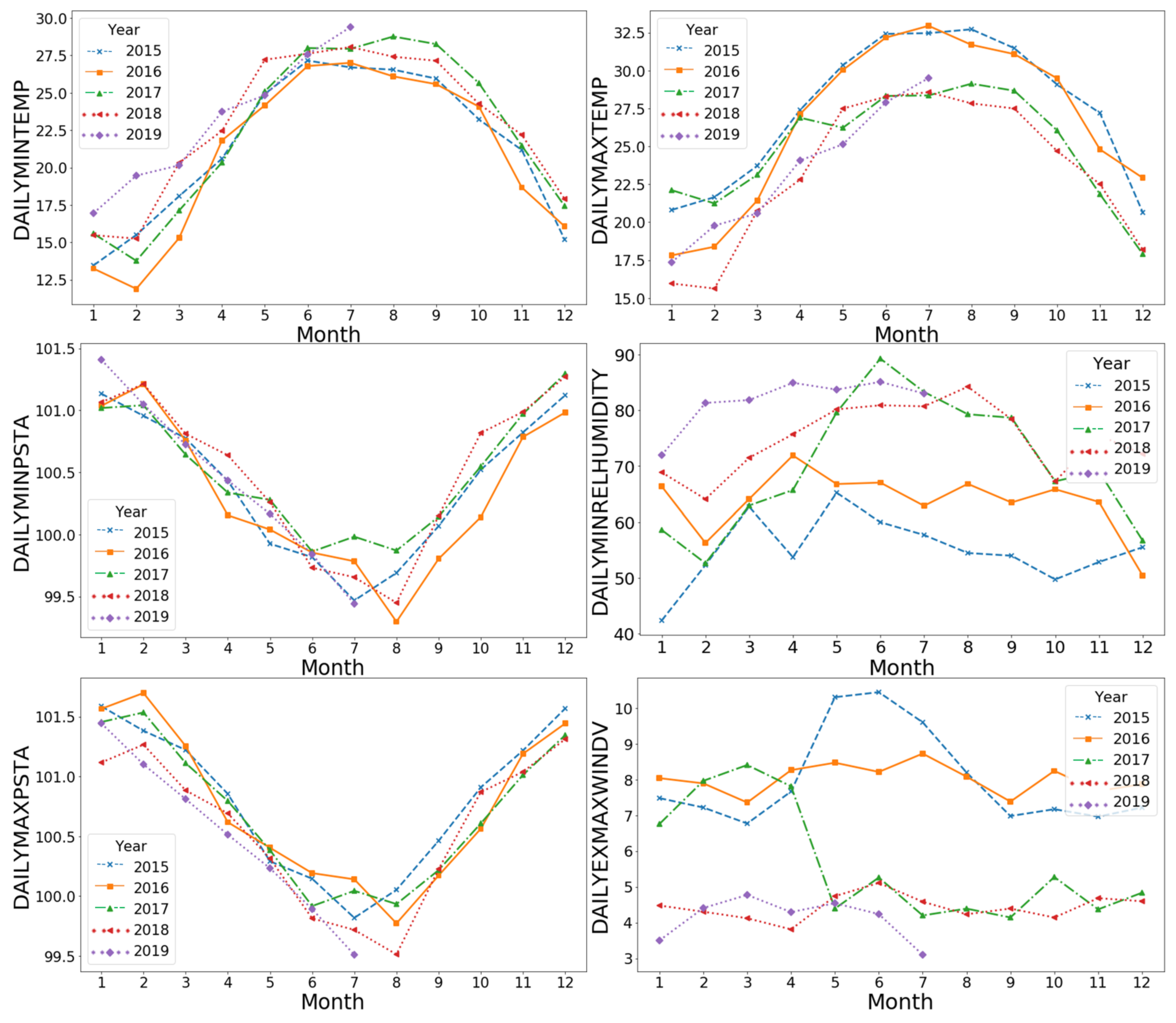
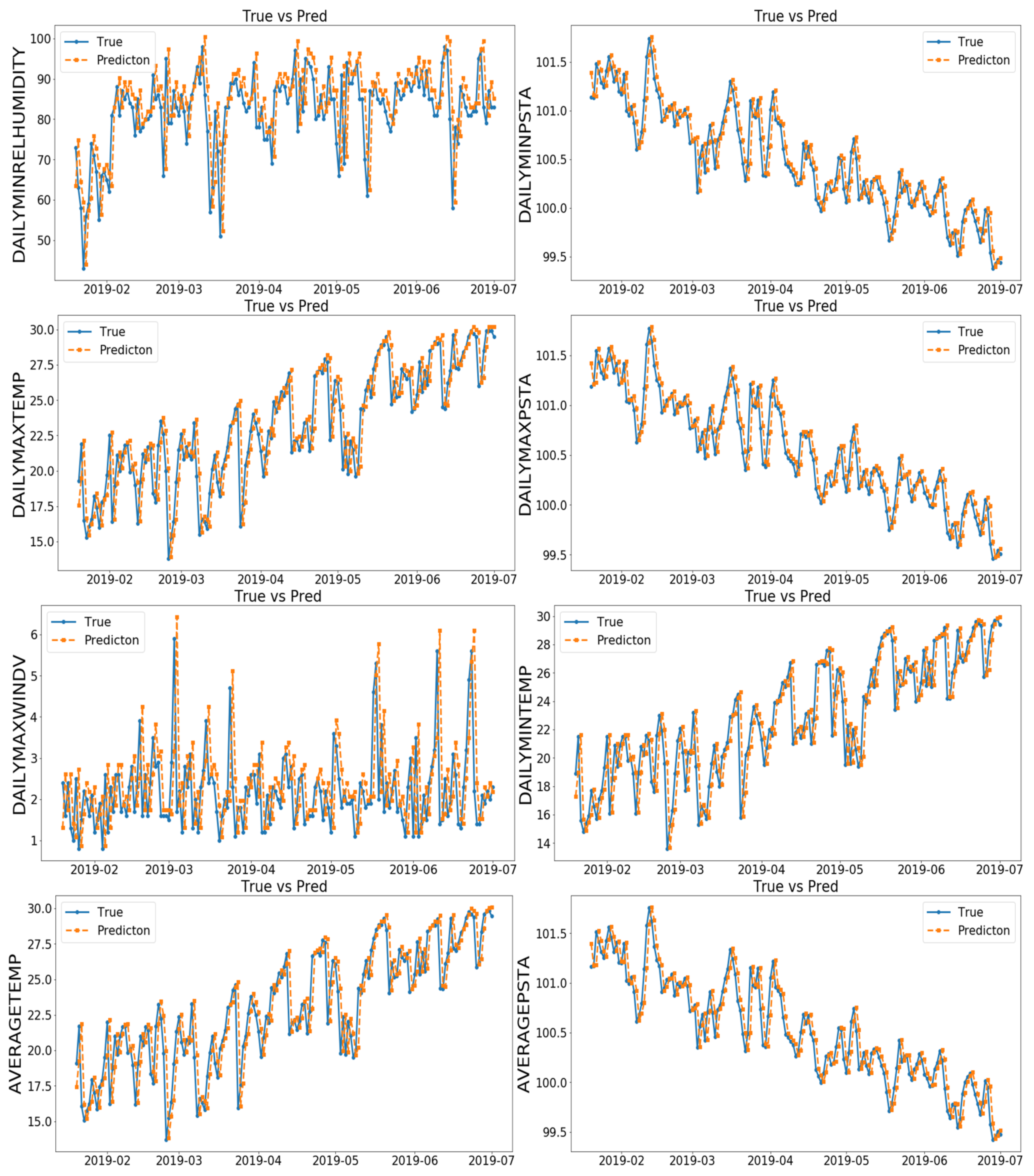
The meteorological conditions of Shenzhen are changeable, often with “sudden warm and cold” weather and a lack of relevant weather research. In this paper, the EMD-LSTM model was used to forecast the daily weather conditions of Shenzhen city by analyzing the historical weather data and related experiments. In order to reduce the use of a single machine learning method to predict the characteristics of a data error, this paper used empirical mode decomposition (EMD) on the various characteristics of weather data noise reduction decomposition, with stability and with different frequencies of multiple components and a residual error sequence, and picked out the greater influence on the characteristics of the original sequence to merge the data. Combined with the long- and short-term memory neural network (LSTM) in deep learning, multivariable forecasting was realized, so as to provide more accurate prediction of the minimum humidity, minimum air pressure, maximum temperature, maximum air pressure, maximum wind speed, minimum temperature, average temperature, average pressure and minimum temperature of daily weather conditions in Shenzhen.

2. Data and Methods

2.1. Data

The data source of this paper is the daily data of Shenzhen published by Shenzhen Meteorological Bureau (https://opendata.sz.gov.cn// accessed on 27 July 2022), the data collection of the statistics from 2015–2019 Shenzhen daily weather conditions of minimum humidity (%), minimum air pressure (Kpa), maximum temperature (°C), maximum air pressure (Kpa), maximum wind speed (0.1 m/s) and minimum temperature (°C). According to the data set, EMD method was used to decompose the weather indicators one by one. After selecting variables by Pearson coefficient, the data were reconstructed and input into LSTM network to achieve multivariable forecasting. Figure 1 shows the monthly data trend of daily meteorological indicators in the past five years. The sequence has obvious correlation and seasonal trend.

2.2. EMD Method

Empirical mode decomposition (EMD) was proposed by Dr. Huang et al. in 1998 [20]. It is an adaptive time-frequency signal processing method, which can eliminate the non-stationarity of sequence and extract the trend of data [21]. This method breaks the limitation of the traditional data method which needs to set the basis function in advance and has more obvious advantages than the traditional smoothing method [22]. Each signal is decomposed into stationary sequences of different feature scales, and each stationary sequence is an intrinsic modal function (IMF) containing different feature scales of the original signal. Among them, each IMF component must meet two conditions at the same time: the number of original signal extreme points crossing zero is equal to or different by one; at any time, the average of the upper and lower envelope of the original signal must be zero. The steps of EMD decomposition for any original time-series signal to be processed are as follows:
(1)
According to the upper and lower extreme value points of the original signal, the upper and lower envelope lines are calculated respectively by using cubic spline interpolation, and the mean value of the upper and lower envelope lines is calculated, as shown in Formula (1).
m 1 ( t ) = 1 / 2 ( U ( t ) + L ( t ) )
(2)
According to Formula (2), the intermediate signal is obtained by subtracting the original signal from the mean envelope.
h 1 ( t ) = X ( t ) m 1 ( t )
(3)
The intermediate signal of h 1 ( t ) is obtained according to Formula (2), denoted as h 11 ( t ) , where m 11 ( t ) is the mean envelope of h 1 ( t ) . Normally, the process iterates k times until the resulting intermediate signal h 1 ( t ) meets the IMF condition. According to Formula (3), SD represents the standard deviation of the intermediate signal of two consecutive iterations where k represents the number of iterations, and h 1 k ( t ) represents the intermediate signal obtained in the Kth iteration. According to Dr. Huang, SD is set to 0.2–0.3.
SD = t = 0 T [ | h 1 ( k 1 ) ( t ) h 1 k ( t ) | 2 h 1 ( k 1 ) 2 ( t ) ]
(4)
Using above method, obtain the first IMF postscript for c 1 ( t ) , then c 1 ( t ) from the original signal; obtain allowance for r 1 ( t ) ; due allowance r 1 ( t ) still contains a large amount of information, thus the r 1 ( t ) as new original signal; repeat the above steps to obtain r n ( t ) = r ( n 1 ) ( t ) c n ( t ) .
When c n ( t ) or r n ( t ) is less than a predetermined value, or R is a monotone function and cannot extract more IMF, the iteration is terminated. The final decomposition result is Formula (4), where r n ( t ) represents the central tendency of the original sequence, and c n ( t ) represents the characteristic performance of the original sequence on different scales.
X ( t ) = i = 1 n c i ( t ) + r n ( t )

2.3. LSTM Method

The model structure of long short-term memory network (LSTM) was proposed by Professor Hochreiter in 1997 [23]. LSTM network structure is a neural network model of recurrent neural network (RNN) formed by adding different gating units in the hidden layer, which has longer short-term memory, stronger memory ability and better processing of long serial number signal data. It enables the recurrent neural network to effectively utilize the training data in a wide range, thus improving the performance of the model. The internal department control structure of LSTM network is shown in Figure 1.
g f = σ ( W f [ h t 1 , x t ] + b f )
Figure 2 shows the structure of an LSTM cell. LSTM uses three gates: input gate, forget gate and output gate to control the flow of internal information. The forget gate acts on the LSTM state vector c t , which represents the input of long-term memory c t 1 and is used to control the influence of the memory of the last time on the current time. The control variable g f of the forget gate is generated by Formula (5) where W f and b f represent weights and bias and which is the activation function.
The input gate is used to control LSTM’s reception of input, and a new input vector c ˜ t is obtained by nonlinear transformation of the input x t at the current time and the output h t 1 at the last time, which is used to control the input range within the range [−1, 1]. The control variable g i of the input gate also comes from input x t and output h t 1 , as shown in Formula (6).
g i = σ ( W i [ h t 1 , x t ] + b i )
Under the control of the forgetting gate and the input gate, LSTM selectively reads the last memory information c t 1 and the new input c ˜ t of the current time. The refreshing mode of state vector c t is shown in Formula (7).
c t = g i c ˜ t + g f c t 1
At this time, the state vector is selectively output under the action of the output gate. In Formula (8), it is determined by the gating variable g 0 of the output gate. The output of LSTM is generated by Formula (9). Since g 0 [ 0 , 1 ] and tanh ( c t ) [ 1 , 1 ] , the output h t [ 1 , 1 ] of LSTM is obtained.
g o = σ ( W o [ h t 1 , x t ] + b o )
h t = g o tanh ( c t )

3. Research Design

3.1. Construction of EMD-LSTM Combined Model

The data collected by the telemetry station of the meteorological station are various, complicated and noisy. To solve this problem, this paper proposes a forecast model combining EMD decomposition and the LSTM network. After data outliers are processed, the characteristic values with a high correlation coefficient with the target value are screened out from the original data set by Pearson’s correlation coefficient. After the combination of components with high correlation with characteristic values is obtained through EMD decomposition, the key sequences that mainly affect the target values are determined and input into the LSTM network for the training model, and the final forecast results are obtained. The EMD-LSTM combined model is shown in Figure 3.

3.2. Design of Forecast Model

Daily weather data of Shenzhen from 1 January 2015 to 1 January 2019 were selected. The data of missing values were supplemented by means of upper and lower data, normalized data were processed, and the target values were decomposed by EMD (here, the minimum temperature was taken as an example, and other meteorological indicators were consistent with the processing process). The decomposed variables were recombined with the original data according to Pearson’s correlation coefficient as the input data set. This paper used a deep learning network and Python software based on the Tensorflow platform. The LSTM model structure of the design in this paper is composed of three layers of an LSTM network layer upon layer overlay, with depth to extract data information, and finally, the forecasted output is connected by a whole structure, the LSTM structure used for extracting features, depth of extraction of the data characteristics of the weather conditions and the connection layer for the final fitting; it combines the LSTM model to extract the characteristics of the forecast, and results are obtained. According to the characteristics of weather conditions, sequence data of seven steps are used to forecast the next sequence. The LSTM network structure has three hidden layers with 50 neurons in each layer. The structure of each node is shown in Figure 1. The learning rate of each layer is 0.1, and the forecasted value of the output layer is output after the fully connected layer.

3.3. Optimization of Forecast Model

When optimizing a model to improve model training efficiency and prediction accuracy, grid search (GS) and cross validation (CV) are used to determine the optimal hyperparameter combination of the model, and the Adam optimization algorithm is used to determine the optimal weight and bias of the model. Too many layers or too many elements of hyperparameter LSTM layers, elements and fully connected layers will result in overfitting, while too small a value will result in underfitting. The value of memory duration will affect the training speed and accuracy of the model. Optimization of hyperparameters by GS-CV was conducted. All possible parameters were randomly and freely combined by grid search, the parameters were optimized by the cross-validation method, and the loss function of each cycle was calculated to obtain the optimal parameters. The loss function selected here was the mean absolute error function, and the model parameter combination with the minimum MAE was selected. Then the training model with optimal parameter combination was determined, and then the model was used to verify the error between the real value and the predicted value.
For the optimization of the model, the Adam algorithm was used to optimize the gradient descent algorithm, which dynamically adjusts the learning rate of each parameter by using the first- and second-moment estimation of the gradient. The weight of the LSTM model and the updated value Δ θ t of bias are calculated by the following formula one by one where G t represents the gradient at time t; μ and ν represent the decay rate of the distance estimate, generally, μ = 0.9 , ν = 0.999 ; and m ^ t and n ^ t are corrections to m t and n t , which can be approximated as unbiased estimates of expectations.
{ m t = μ m t 1 + ( 1 μ ) G t n t = ν n t 1 + ( 1 ν ) G t 2
{ m ^ t = m t 1 μ t n ^ t = m t 1 ν t
Δ θ t = m ^ t n ^ t + ε η
Figure 4 shows the flow chart of the Adam algorithm. Firstly, the first moment and second moment n t of gradient G t are calculated by using Equation (10), and then the first-moment estimation deviation m ^ t and second-moment estimation deviation n ^ t are corrected according to Equation (11). Finally, the bias correction Δ θ t of the weight of the LSTM model is obtained by using Equation (12), where η is the step size and is the small constant of the stable value. Generally, η = 0.001 , ε = 10 8 .

3.4. Evaluation Method of Model Forecast Effect

When different forecast models are used for quantitative analysis and evaluation, the mean square error (MSE), root mean square error (RMSE) and mean absolute error (MAE) of evaluation indexes are used to evaluate the accuracy and stability of the model forecast, and their calculation is shown in Formulas (13)–(15).
MSE = 1 m i = 1 m ( y test i y ^ test i ) 2
RMSE = 1 m i = 1 m ( y test i y ^ test i ) 2
MAE = 1 m i = 1 m | ( y test i y ^ test i ) |
where y i and y ^ i represent the real value and predicted value of a single sequence, respectively. MSE represents the sum of squares of the deviation between the predicted value and the true value. Compared with MSE, RMSE has the same dimension as the original data and represents the square root of the ratio of the deviation between the predicted value and the real value and the number of predicted tests, which reflects the deviation between the real value and the predicted value. MAE represents the average absolute value of the error and represents the actual size of the prediction error. The smaller the three evaluation indexes, the more accurate the model’s predictions are.

4. Experiment and Analysis

4.1. Data Preprocessing

A correlation test between variables can be realized by the KMO test. The closer the KOM statistic is to 1, the stronger the correlation between variables is, and the weaker the partial correlation is. It can be seen from Table 1 that the KMO test values of all variables are greater than 0.6, indicating that there is a high correlation between all-weather variables. Therefore, multivariable prediction has a reliable basis.
Each component of six features was obtained through EMD decomposition, and correlation coefficient analysis was carried out between the decomposed feature and all components decomposed. Taking the minimum temperature as an example, EMD decomposition of the minimum temperature was performed to obtain eight IMF decomposition variables and a residual sequence, as shown in Figure 5.
The Pearson coefficient of each component and the minimum temperature of the original sequence can be calculated by using Formula (16) of decomposed components and the minimum temperature, and the variables highly correlated with the minimum temperature can be screened out.
R = 1 n 1 i = 1 n ( x i x ¯ s x ) ( y i y ¯ s y )
As shown in Table 2, the correlation coefficients between the original sequence of the lowest temperature and IMF6 and IMF5 reached 0.822 and 0.510, indicating that these two components had a great relationship with the original sequence. Therefore, two indexes IMF6 and IMF5 were selected from all the components and then combined with the remaining original indexes and input into the LSTM model to forecast the minimum temperature with multiple variables. All other features are the same as the minimum temperature prediction procedure.

4.2. Effect of Model

In this paper, data from 1 January 2015 to 15 January 2019 were selected as the training set, and data from 16 January 2019 to 7 July 2019 were selected as the verification set. Data from 16 January 2019 to 7 July 2019 were used as validation sets. Based on the optimal parameters obtained from the model optimization above, the superiority of the EMD-LSTM combined model designed in this paper was verified. The LSTM model, CNN model and EMD-LSTM model were used for comparative experiments, and the three models all converged in 20 iterations, among which the EMD-LSTM model had the fastest convergence speed and reached a stable state in the seventh iteration with the smallest error. The LSTM model reached a stable state in the 12th iteration, and the error was smaller than that of the CNN model. The CNN model reached a stable state in the 15th iteration, with the largest error among the three models. Figure 6 visually shows the small error between the predicted value and the real value of each indicator in the validation set of the EMD-LSTM model. It can be seen that the predicted value of the model is close to the real value and the prediction effect is good.
It can be seen from Table 3 that the mean square error, root mean square error and mean absolute error of the EMD-LSTM model are all minimum, which shows that the model designed in this paper is suitable for weather prediction. The mean error MSE, RMSE and MAE of the model designed by us are 0.0435, 0.1216 and 0.0654, respectively. Compared with the original LSTM model and CNN model, The MSE value of the EMD-LSTM model is reduced by 1.92% and 4.12% on average, the RMSE value is reduced by 3.11% and 16.69% on average, and the MAE value is reduced by 6.15% and 16.26% on average. Therefore, among the basic models in deep learning, the EMD-LSTM model has the best effect and the least error.
The comparison between our model and the traditional machine learning models, namely the random forest (RF) and support vector machine (SVM) models, is shown in Table 4. It can be seen from Table 4 that the mean square error, root mean square error and mean absolute error of our model still are all minimum. The daily humidity prediction errors of RF and SVM are both large, while the overall mean error of RF is smaller.
The comparison between our model and regression models, namely the multiple linear regression (MLR), support vector regression (SVR), polynomial regression and ridge regression models, is shown in Table 5 and Table 6. As can be seen from Table 5 and Table 6, the mean square error, root mean square error and mean absolute error of our model are still the smallest. The daily humidity prediction errors of the four regression models are all large, but ridge regression is the best among the four regression models because of its minimum overall mean error.

5. Conclusions

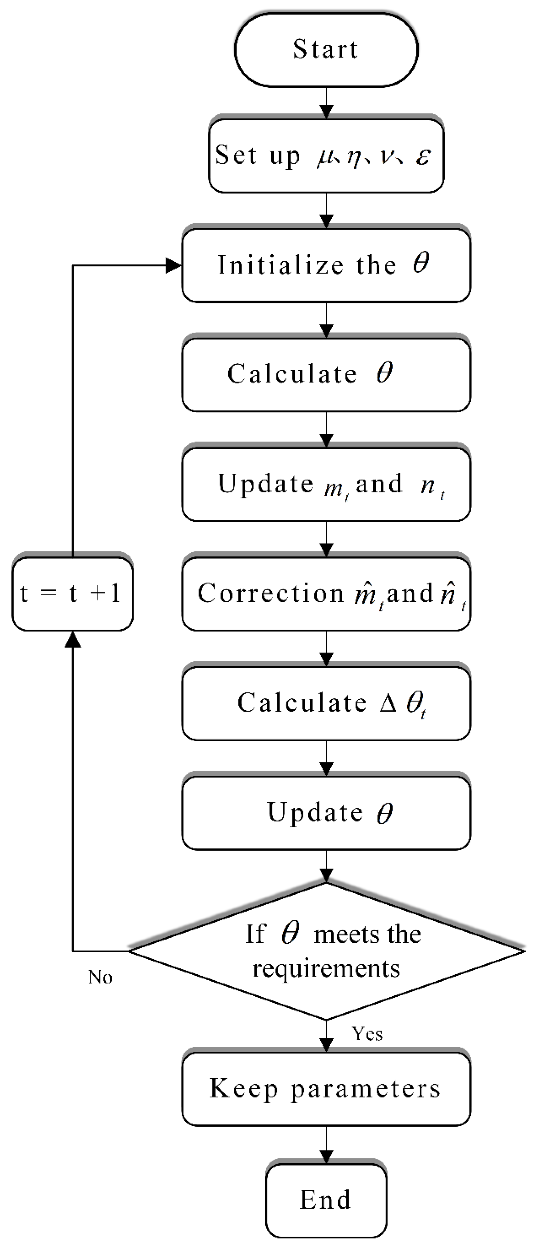
In order to improve the accuracy of weather forecasts, this paper proposes a fusion model based on a deep learning neural network of long and short memory. The minimum humidity, minimum air pressure, maximum temperature, maximum air pressure, maximum wind speed, minimum temperature, average temperature and average pressure were predicted under daily weather conditions in Shenzhen, China. The method of filtering the correlation coefficients of the components of each variable decomposed by EMD and then recombining the data into an LSTM network makes full use of the advantages of EMD in the decomposition of non-stationary data with seasonal trends and reduces the influence of data noise and seasonal fluctuations. Combined with the LSTM model, it has the advantage of “memory ability and forgetting ability” in time-series data processing, the grid search is used to find the optimal combination of hyperparameters, and the gradient descent optimization algorithm is used to find the optimal weight and bias of the model, so as to improve the prediction accuracy of Shenzhen’s weather characteristics. Four kinds of traditional machine learning models and four Kernel regression model experiments fully prove that the EMD-LSTM combined model designed in this paper is a more efficient and accurate model, which is suitable for weather prediction and can provide new ideas for weather prediction.

Author Contributions

Data curation, F.J.; Funding acquisition, G.C.; Investigation, S.L.; Methodology, G.C. and S.L.; Supervision, F.J.; Writing—original draft, S.L.; Writing—review & editing, G.C. All authors have read and agreed to the published version of the manuscript.

Funding

The study was supported by the National Natural Science Foundation of China (11701304) and the Natural Science Foundation of Ningbo City (2019A610041).

Institutional Review Board Statement

Not applicable.

Informed Consent Statement

Not applicable.

Data Availability Statement

Data available in a publicly accessible repository that does not issue DOIs. Publicly available datasets were analyzed in this study. This data can be found here: https://opendata.sz.gov.cn// accession on 27 July 2022.

Conflicts of Interest

The authors declare no conflict of interest.

References

  1. Wei, X.L.; Liu, Y.W.; Liu, Y.B.; Li, L. Numerical study of a local PM2.5 pollution event under the typhoon Neoguri (1408) background over a coastal metropolitan city, Shenzhen, China. Phys. Chem. Earth 2019, 110, 99–108. [Google Scholar] [CrossRef]
  2. Jiang, Z.; Yang, S.; Liu, Z.; Xu, Y.; Xiong, Y.; Qi, S.; Pang, Q.; Xu, J.; Liu, F.; Xu, T. Coupling machine learning and weather forecast to predict farmland flood disaster: A case study in Yangtze River basin. Environ. Model. Softw. 2022, 155, 1364–8152. [Google Scholar] [CrossRef]
  3. Qian, K.; Tian, X.; Bricker, J.; Zhan, T. Urban pluvial flooding prediction by machine learning approaches a case study of Shenzhen city, China. Adv. Water Resour. 2020, 145, 1679–1708. [Google Scholar]
  4. Liu, Z.; Xie, M.; Tian, K. Gao PGIS-based analysis of population exposure to PM25 air pollution—A case study of Beijing. J. Environ. Sci. Clim. Chang. Urban Environ. 2017, 59, 48–53. [Google Scholar]
  5. Cobourn, W.G. An enhanced PM2.5 air quality forecast model based on nonlinear regression and back-trajectory concentrations. Atmos. Environ. 2010, 44, 3015–3023. [Google Scholar] [CrossRef]
  6. Ni, X.Y.; Huang, H.; Du, W.P. Relevance analysis and short-term prediction of PM2.5 concentrations in Beijing based on multi-source data. Atmos. Environ. 2017, 150, 146–161. [Google Scholar] [CrossRef]
  7. Zeng, L.; Hang, J.; Wang, X.; Shao, M. Influence of urban spatial and socioeconomic parameters on PM2.5 at subdistrict level: A land use regression study in Shenzhen, China. J. Environ. Sci. 2022, 114, 485–502. [Google Scholar] [CrossRef]
  8. Chen, J.L.; Chen, P.B.; Tingting, J. Application analysis of meteorological Big data Service in cloud computing Environment. China Sci. Technol. Inf. 2019, 11, 88–90. [Google Scholar]
  9. Huang, J. ARIMA Short-term wind speed Prediction based on Extreme Value migration optimization. Manuf. Autom. 2018, 40, 79–85. [Google Scholar]
  10. Bao, Y.S.; Wu, Z.S.J. Time series short-term wind speed prediction based on SVM. China Electr. Power 2011, 44, 61–64. [Google Scholar]
  11. Tao, Y.; Du, J.L.J. Long-term and short-term memory network temperature prediction based on random forest. Comput. Eng. Des. 2019, 40, 737–743. [Google Scholar]
  12. Gong, B.M.; Wang, W.B.; Zhao, P.J. EMD—FSV prediction for non stationary time series. Comput. Sci. 2014, 41, 57–60. [Google Scholar]
  13. Motin, M.A.; Karmakar, C.K.; Palaniswami, M. Selection of empirical mode decomposition techniques for extracting breathing rate from PPG. IEEE Signal Process. Lett. 2019, 26, 592–596. [Google Scholar] [CrossRef]
  14. Qi, Y.Y.; Yu, M.J. Anti-jamming method for frequency hopping communication based on single channel BSS and EMD. Comput. Sci. 2016, 43, 149–153. [Google Scholar]
  15. Zheng, D.; Cui, G.; Cao, J.; Tanaka, T. Analysis of brain-death EEG data using 2T-EMD algorithm. In Proceedings of the 2015 11th International Conference on Signal-Image Technology & Internet-Based Systems (SITIS), Bangkok, Thailand, 23–27 November 2015. [Google Scholar]
  16. Tian, Z.; Li, H.; Li, F. A combination forecasting model of wind speed based on decomposition. Energy Rep. 2021, 7, 1217–1233. [Google Scholar] [CrossRef]
  17. Zhang, Y.; Pan, G.; Chen, B.; Han, J.; Zhao, Y.; Zhang, C. Short-term wind speed prediction model based on GA-ANN improved by, V.M.D. Renew. Energy 2020, 156, 1373–1388. [Google Scholar] [CrossRef]
  18. Tian, Z.; Chen, H. A novel decomposition-ensemble prediction model for ultra-short-term wind speed. Energy Convers. Manag. 2021, 248, 114775. [Google Scholar] [CrossRef]
  19. Yang, L.; Liu, C.H.; Gou, Y.C.; Deng, H.J.; Li, D.L.; Duan, Q.L. Prediction of ammonia concentration in piggery based on EMD-LSTM. Trans. Chin. Soc. Agric. Mach. 2019, 50, 353–360. [Google Scholar]
  20. Huang, N.E.; Shen, Z.; Long, S.R.; Wu, M.C.; Shih, H.H.; Zheng, Q.; Yen, N.-C.; Tung, C.C.; Liu, H.H. The empirical mode decomposition and the hilbert spectrum for nonlinear and non-stationary time series analysis. Proc. R. Soc. London. Ser. A Math. Phys. Eng. Sci. 1998, 454, 903–995. [Google Scholar] [CrossRef]
  21. Wang, W.B.; Zhang, X.D.; Wang, X.L. Empirical mode decomposition denoising method based on principal component analysis. Acta Electron. Sin. 2013, 41, 1425–1430. [Google Scholar]
  22. Mao, Y.L.; Fan, H.J. Review and prospect of empirical mode decomposition. Comput. Eng. Sci. 2014, 1, 155–162. [Google Scholar]
  23. Hochreiter, S.; Schmidhuber, J. Long Short-Term Memory. Neural Comput. 1997, 9, 1735–1780. [Google Scholar] [CrossRef] [PubMed]
Figure 1. The monthly data trend of daily meteorological indicators in the past five years.
Atmosphere 13 01208 g001
Figure 2. LSTM structure.
Atmosphere 13 01208 g002
Figure 3. EMD-LSTM.
Figure 3. EMD-LSTM.
Atmosphere 13 01208 g003
Figure 4. Adam algorithm flow.
Atmosphere 13 01208 g004
Figure 5. Daily minimum temperature of the EMD decomposition.
Atmosphere 13 01208 g005
Figure 6. The predicted values and the actual value error.
Atmosphere 13 01208 g006
Table 1. KMO test value.
FeatureMinrelhumidityMaxtempMaxpstaExmaxwindvMintempMinpsta
KMO0.8120.8270.7900.6610.8080.606
Table 2. Pearson coefficient.
ComponentPearson Coefficient
IMF10.278
IMF20.278
IMF30.226
IMF40.202
IMF50.510
IMF60.822
IMF70.093
IMF80.031
r0.178
Table 3. Error comparison results of deep learning model.
FeatureMSERMSEMAE
LSTMCNNOURLSTMCNNOURLSTMCNNOUR
Minrel-humidity0.03040.08650.01170.17440.29410.10820.12500.23400.0828
Minpsta0.00010.08540.00000.00410.29220.00330.03080.22880.0036
Maxtemp0.02870.08530.00910.16730.29200.09570.22070.23090.0974
Maxpsta0.00170.08460.00020.00410.29090.01470.00410.22910.0099
Exmaxwindv0.41640.08360.30880.64530.28920.55770.42270.22690.1873
Mintemp0.01170.08700.00930.10830.29500.09630.13290.23120.0702
Averagetemp0.01240.08270.00900.11140.27760.09500.07470.22180.0701
Averagepsta0.00000.08230.00000.00690.27670.00210.00450.22130.0017
Mean error0.06270.08470.04350.15270.28850.12160.12690.22800.0654
Table 4. Error comparison results of traditional machine learning models.
FeatureMSERMSEMAE
RFSVMOURRFSVMOURRFSVMOUR
Minrel-humidity63.1064270.80460.01177.944016.45610.10826.086813.07280.0828
Minpsta0.03690.66650.00000.19220.81640.00330.07120.66190.0036
Maxtemp0.281528.98500.00910.53055.38380.09570.53054.38650.0974
Maxpsta0.03860.48800.00020.19660.69860.01470.15200.57890.0099
Exmaxwindv0.672028.13320.30880.81975.30410.55770.81974.32210.1873
Mintemp0.329729.57610.00930.57425.43840.09630.38254.46700.0702
Averagetemp0.860827.17070.00900.92785.21260.09500.70924.25000.0701
Averagepsta0.10320.43260.00000.32120.65770.00210.25300.55250.0017
Mean error8.180048.28210.04351.43834.99600.12161.12564.03650.0654
Table 5. Error comparison results of regression models (a).
FeatureMSERMSEMAE
MLRSVROURMLRSVROURMLRSVROUR
Minrel-humidity76.6398270.80460.01178.754416.45610.10826.9339813.07280.0828
Minpsta5.40370.66650.00002.32460.81640.00331.81910.66190.0036
Maxtemp0.271828.98500.00910.51375.38380.09570.36264.38650.0974
Maxpsta0.03710.48800.00020.19260.69860.01470.14390.57890.0099
Exmaxwindv1.018228.13320.30881.00915.30410.55770.79164.32210.1873
Mintemp0.278929.57610.00930.52815.43840.09630.35154.46700.0702
Averagetemp1.153827.17070.00901.07415.21260.09500.85714.25000.0701
Averagepsta0.12820.43260.00000.35810.65770.00210.28110.55250.0017
Mean error10.616448.28210.04351.78014.99600.12161.39734.03650.0654
Table 6. Error comparison results of regression models (b).
FeatureMSERMSEMAE
PolynomialRidgeOURPolynomialRidgeOURPolynomialRidgeOUR
Minrel-humidity51.382574.38120.01177.16828.62450.10825.32786.59120.0828
Minpsta33.35864.57630.00005.77572.13920.00333.73701.59690.0036
Maxtemp1.05080.01110.00911.02510.10530.09570.69600.07390.0974
Maxpsta0.00520.04130.00020.07190.20320.01470.05220.15930.0099
Exmaxwindv1.02631.14210.30881.01311.06870.55770.78430.83880.1873
Mintemp1.02630.02280.00931.01310.01510.09630.78430.01100.0702
Averagetemp1.51470.02950.00903.89190.05430.09502.97770.08060.0701
Averagepsta0.04450.00000.00000.21090.00010.00210.16470.00010.0017
Mean error11.176110.02550.04352.52121.52630.12161.81551.16900.0654
Publisher’s Note: MDPI stays neutral with regard to jurisdictional claims in published maps and institutional affiliations.

