Article

Analysis of Pre-Earthquake Space Electric Field Disturbance Observed by CSES

1
Key Laboratory of Building Collapse Mechanism and Disaster Prevention, Institute of Disaster Prevention, China Earthquake Administration, Langfang 065201, China
2
Institute of Disaster Prevention, Institute of Intelligent Emergency Information Processing, Langfang 065201, China
3
Institute of Disaster Prevention, School of Emergency Management, Langfang 065201, China
4
National Institute of Natural Hazards, Ministry of Emergency Management of China, Beijing 100085, China
5
Institute of Disaster Prevention, School of Information Engineering, Langfang 065201, China
*
Author to whom correspondence should be addressed.
Atmosphere 2022, 13(6), 934; https://doi.org/10.3390/atmos13060934
Submission received: 18 May 2022 / Revised: 3 June 2022 / Accepted: 6 June 2022 / Published: 9 June 2022
(This article belongs to the Special Issue Ionospheric Science and Ionosonde Applications)

Abstract

:
In order to explore the abnormal disturbance of the space electric field caused by earthquakes using the electric field data of the ULF and VLF frequency bands of the electric field observed by the ZH-1 satellite, and taking the Mw7.7 earthquake in the Caribbean Sea in the southern sea area of Cuba on 29 January 2020 as an example, the signal-to-noise ratio of the NAA and NLK artificial source VLF transmitting stations in the Northern Hemisphere and the height of the lower ionosphere was calculated. The disturbance of the electric field in the ULF band was extracted using the S-G filtering method. The results indicate that: (1) The ionospheric anomaly caused by this earthquake appeared 20 days before the earthquake, and before the earthquake, there were significant anomalous changes in all parameters within the pregnant seismic zone. The signal-to-noise ratios of the NAA and NLK artificial source transmitter stations decreased by 30%, and the height of the low ionosphere decreased by 5–10 km, while there were anomalous perturbations in several orbits of the ULF electric field, and the magnitude of the perturbations exceeded three times the standard deviation. (2) The SNR of the artificial source transmitting stations before and after the earthquake was significantly reduced in the third period before the earthquake and recovered after the earthquake. (3) The low ionospheric height appears to be reduced before the earthquake and recovers after the earthquake. (4) The decrease in the S/N ratio occurred simultaneously with the decrease in ionospheric height 15 days–10 days before the earthquake. This provides a reference for extracting pre-earthquake ionospheric precursor anomalies.

1. Introduction

Among all of natural disasters, earthquakes cause the most damage to people and the most serious economic losses. According to the statistics, earthquakes occur about a million times a year [1], causing huge economic losses and seriously affecting people′s productivity, daily life, and the stable development of society. Continental plates squeeze and collide with each other, resulting in dislocation and rupture at the edges of the plates or within the plates. In this process, the Earth′s crust generates seismic waves during a rapid release of energy, which triggers earthquakes. During the gestation process of earthquakes, the generated electromagnetic effects lead to anomalous changes in various ionospheric parameters over the epicenter [2] through the LAI (lithosphere–atmosphere–ionosphere) coupling mechanism, which are recorded by the satellites flying overhead. Therefore, the use of satellites to observe ionospheric disturbances is one of the most promising aspects in seismic research [3]. The process is shown in Figure 1.
Since the first discovery of anomalies in the electromagnetic data observed by satellites before earthquakes [4], studies of ionospheric disturbances using satellites have been widely conducted at domestic and international levels. Studies targeting the spatial electric field including from the DC to HF bands have found pre-seismic electromagnetic disturbance phenomena [5,6,7,8,9]. In the Wenchuan earthquake, researchers then used the DEMETER satellite to discover large anomalous fluctuations in the ULF band before the earthquake [10], and the signal-to-noise ratios in multiple frequency ranges over the epicenter had very different changes before and after the earthquake [11]. In the Yushu earthquake, Zhao et al. found that the reason for the change in the signal-to-noise ratio was closely related to the change in ion density in their study of the seismic-induced decrease in the SNR of artificial source transmitting stations [12]. In order to investigate the mechanism of SNR variations affected by earthquakes, it is necessary to jointly analyze several covariates. The results of previous studies have shown that electromagnetic radiation in the ULF band is generated when rocks collide with each other, leading to rupture [13], and this band signal is almost independent of factors such as weather, lightning, and ionospheric abnormal changes [14]. The VLF band is mainly derived from artificial sources such as strong artificial source signals used for navigation and communication, and is susceptible to space weather effects such as solar activity, rain, snow, lightning, and terrain [15]. Therefore, the joint analytical study of many different covariates can better explain the process of earthquake incubation. In light of this, this paper analyzed the electric field ULF band and VLF band data recorded by the China Seismo-Electromagnetic Satellite (CSES or ZH-1) to study the characteristics of spatial electromagnetic field disturbances in the pre- and post-earthquake periods, and provides a theoretical basis for earthquake monitoring.

2. Background Information

In order to monitor changes in the domestic and surroundings of the Chinese space environment and carry out research on earthquake precursors, China launched a specialized satellite (China Seismo-Electromagnetic Satellite, CSES or ZH-1) for seismic electromagnetic monitoring on 2 February 2018. It has been in orbit for more than four years and has accumulated a large amount of observation data.

2.1. Brief Introduction of ZH-1

The ZH-1 satellite is a geophysical field detection satellite with an operating altitude of about 507 km. It carries eight kinds of loads: High Precision Magnetometer (HPM), Search Coil Magnetometer (SCM), Electric Field Detector (EFD), Plasma Analyzer Package (PAP), Langmuir Probe (LAP), High Energetic Particle Package (HEPP), GNSS Occultation Receiver (GRO), and Tri-Band Beacon (TBB). The revisit period of the satellite is five days and the design life is five years. At present, the satellite operates normally in orbit. According to the scientific research objectives of the CSES and the characteristics of the space electric field environment, the carried EFD was designed with two working modes, which are the BURST mode and SURVEY mode, and four detection bands, and its data products under different working modes are shown in Table 1.
Among them, the BURST mode is to detect the whole area of China and the surrounding areas as well as the Pacific seismic zone and the Eurasian seismic zone, and the working mode for the rest of the region is the SURVEY mode [16,17].

2.2. VLF Artificial Source Transmitter Station

There are many artificial source transmitting stations for communication and navigation all over the world. They continuously transmit VLF band signals, which can penetrate the ionosphere and be received by satellites. The four launch stations in the Americas are listed in Table 2. Electromagnetic waves emitted by strong earthquakes or other interference factors can cause ionospheric disturbances, resulting in abnormal signals observed by satellites [18].
Because the frequencies of the NAU and NML transmitting stations exceeded the effective detection range of the VLF band, the NAA and NLK transmitting stations were selected as the research object in this paper.
According to the empirical formula R = 10 0.43 M , M is the magnitude and R is the radius of the seismogenic zone. The diameter of the earthquake area was calculated to be about 2000 km. The range of ±10° longitude and latitude of the epicenter was selected as the study area. In addition, because the day side of the ionosphere is subject to interference from numerous factors (e.g., solar activity, spacecraft), it is more difficult to capture seismic precursor signals in the ionosphere. Therefore, the electric field data of the night-side ascending orbit were selected for analysis.

3. Multi-Band Signal Joint Analysis of Pre-Earthquake Anomalies

In order to be able to accurately extract the anomalies in different frequency bands of each electric field and to retain the characteristics of the seismogenic signal, the signal-to-noise ratio method was used to extract the signal variations of the artificial source transmitting stations in the VLF band power spectrum data according to the characteristics of the data in different frequency bands, and the residual characteristics were extracted from the ULF band waveform data by S-G filtering, and the low ionospheric height variation in the same period was observed.

3.1. Signal-to-Noise Ratio (SNR) Anomaly Analysis Method

Previous studies have shown that the VLF signal radiating from ground sources can not only penetrate the ionosphere when the energy is strong enough, but can also cause local anomalous changes in the electric field in the ionosphere. In this paper, the signal-to-noise ratio of the VLF artificial source transmitting station in the seismogenic zone was calculated using the SNR method proposed by Molchanov [19]. The SNR equation is as follows.
S N R = 2 A ( f 0 ) A ( f + ) + A ( f )
In Equation (1), A ( f 0 ) is the power spectral density value corresponding to the fixed transmitting frequency of the artificial source transmitting station. A ( f + ) , A ( f ) is the power spectral density value corresponding to the upper and lower frequency limits of the transmitting station, and the bandwidth of the transmitting station frequency is determined by its transmitting power. Figure 2 shows an example of a VLF band that crosses the seismogenic zone orbit.
Two distinct spectral lines can be seen in Figure 2a. The more energetic line in the figure represents the NAA transmitting station (24 kHz), and the weaker line above it represents the NLK transmitting station (24.8 kHz). Figure 2b represents the frequency variation plot of 22–25 kHz at the location of the epicenter at the geographic latitude of 19.4° N. Figure 2 shows that the bandwidth of the NAA transmitting station was about 200 Hz and the bandwidth of the NLK transmitting station was about 100 Hz.

3.2. Analysis of Low Ionospheric Height Variation

Since the British physicist Appleton Leigh discovered the existence of the ionosphere for the first time in 1924 through experiments with artificially emitted signals, research on the propagation of electromagnetic waves in space has been greatly promoted. In the process of earthquake generation, earthquakes cause changes in the height of the lower ionosphere through the LAI coupling mechanism. The height of the lower ionosphere can be calculated by the properties of the electromagnetic wave propagation on the Earth′s surface and in the lower ionosphere [20]. The equation to calculate the height of the lower ionosphere is as follows in Equation (2) [21]:
h = C 2 f c
where h represents the low ionospheric height; C is the speed of light, which is about 300,000 km/s; and f c is the cut-off frequency.

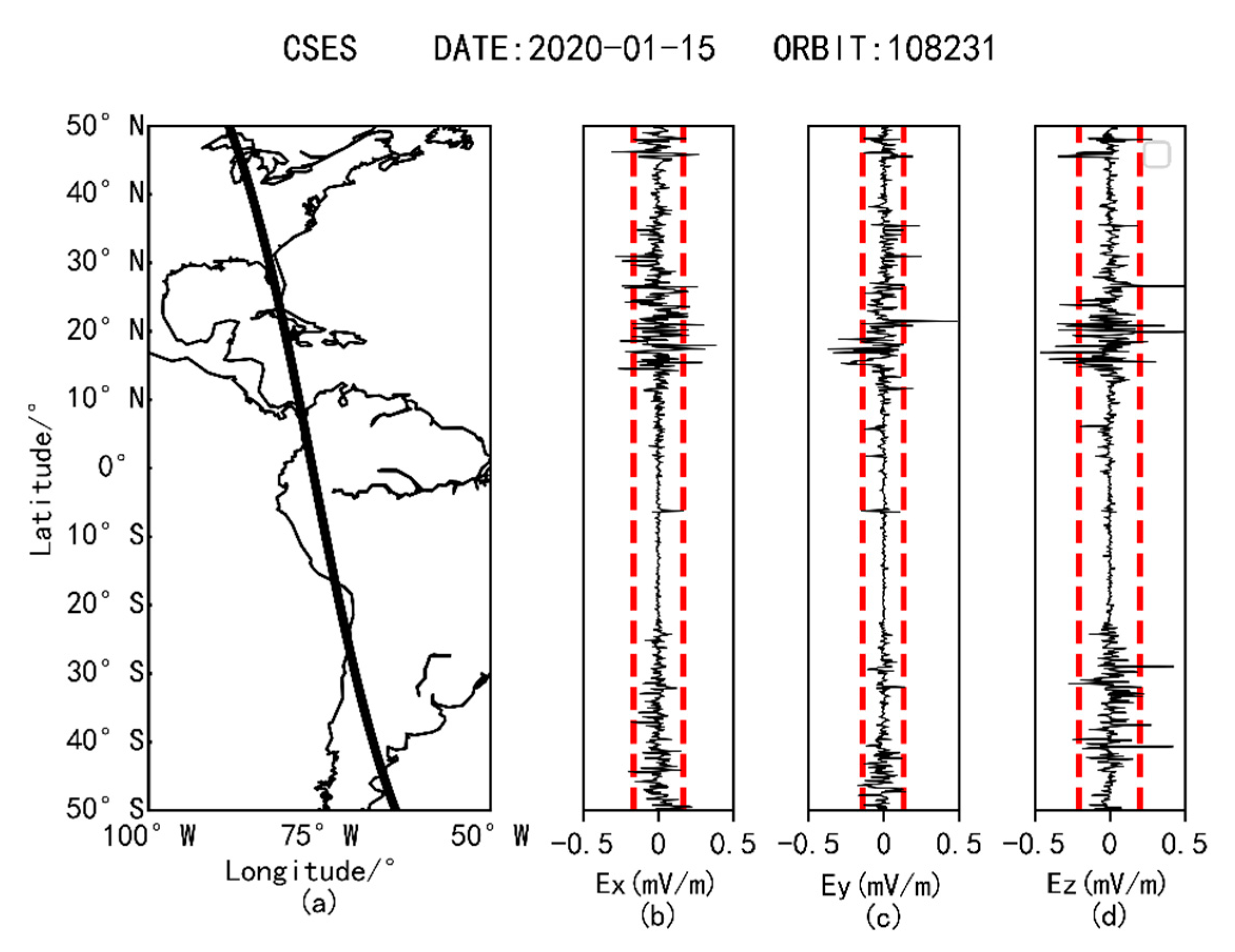
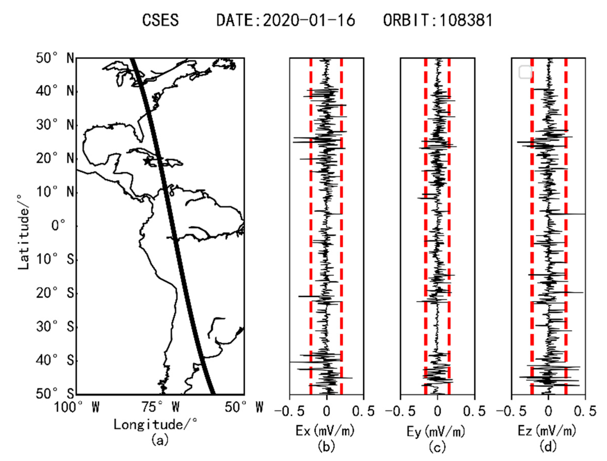
3.3. ULF Band Residual Waveform Anomaly Analysis

The EFD carried by the CSES superimposes the generated V × B electric field with the original electric field signal due to the motion of the satellite cutting the Earth′s magnetic lines of force during the acquisition of the electric field signal, resulting in noise in the observed data of the electric field [22]. To remove this noise signal, the ULF band waveform data are smoothed using a least-squares polynomial smoothing filter denoising algorithm (S-G filter) to obtain its trend waveform [23]. The S-G filter is formulated as follows in Equation (3):
Y j * = i = m i = m C i Y j + i N  
where Yj is the original time series; Y j * is the time series data fit value; C i is the coefficient of the ith time series data value when filtered; N is the number of convolution; j is the coefficient of the original time series data set; and m is the filter window size, which controls the smoothing effect together with the number of smoothing polynomials. The original waveform of the ULF is subtracted from the trend waveform to obtain a set of ULF residual waveforms with the trend signal removed.

4. Earthquake Case Analysis

The Caribbean Sea earthquake occurred on 29 January 2020 at 03:10:22 (UTC), with the epicenter located in southern Cuba (19.46° N, 78.79° W), at a depth of 10 km and a magnitude of Mw7.7. It was a strong earthquake, the largest to occur in the region in the last 100 years. The ionospheric disturbance caused by the ionosphere is obvious and easy to observe. Meanwhile, during the period before and after the earthquake, the CSES operated normally and provided more complete observation data. Second, previous studies have indicated that ionospheric anomalies produced by earthquakes occurring in the ocean are usually not easily observed by satellites, so studying earthquakes occurring in the ocean is very meaningful for the study of seismic ionospheric phenomena. Finally, observing the space weather conditions before and after the earthquake, both geomagnetic and solar activities were normal. Therefore, this seismic event is suitable for studying the ionospheric disturbance phenomenon caused by the earthquake.

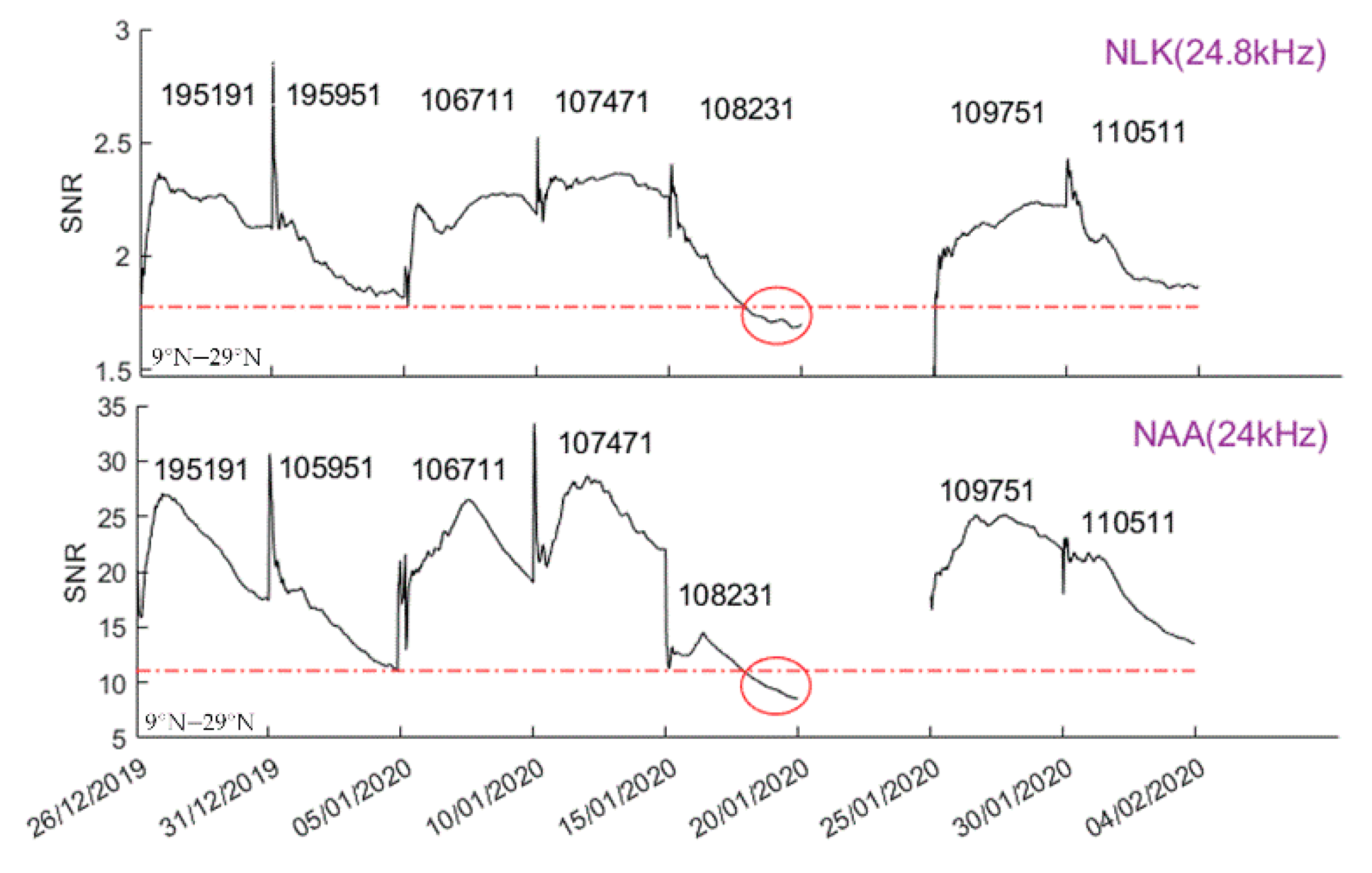
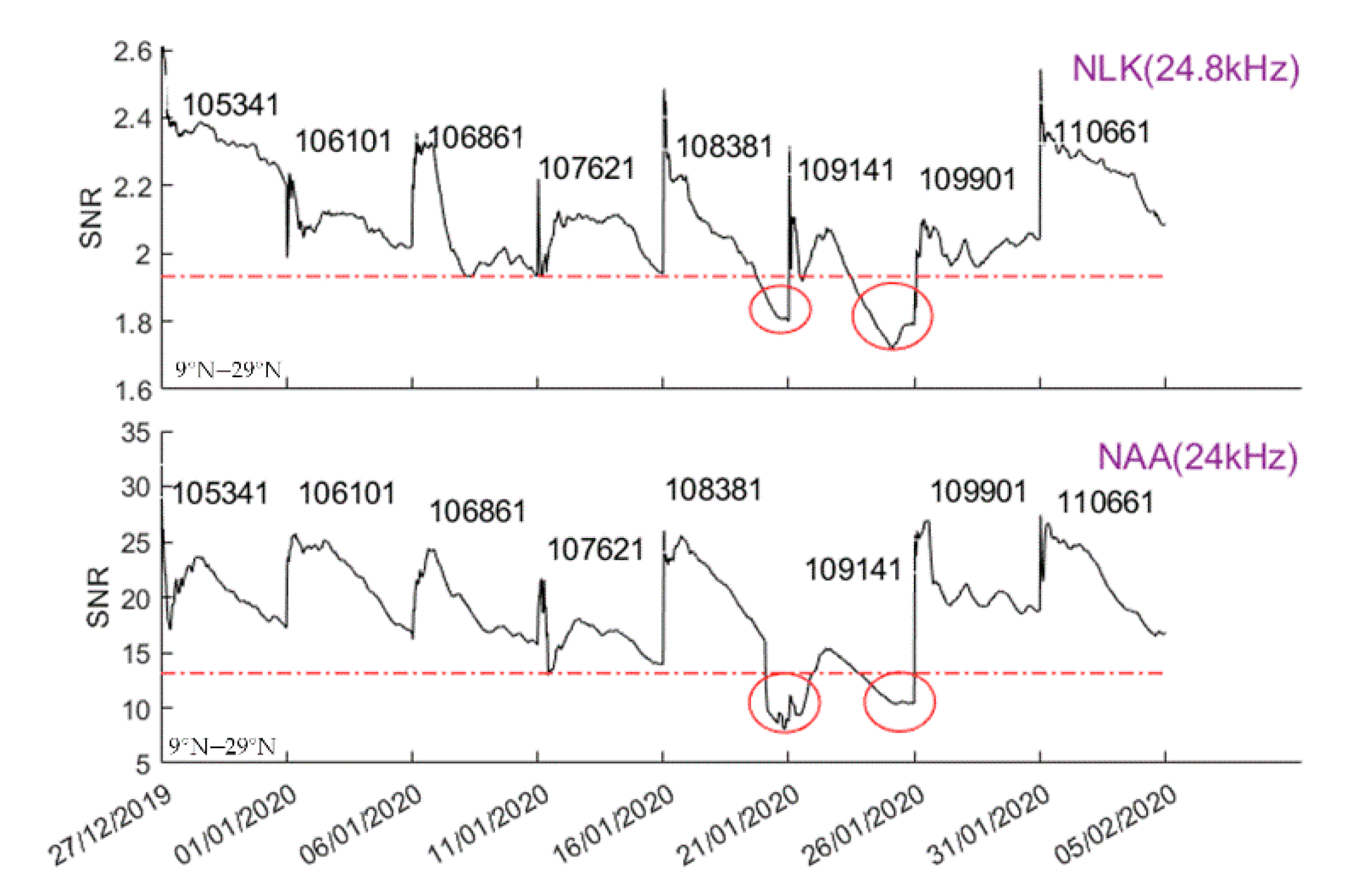
4.1. VLF Transmitting Station SNR

The E-ab component of the 3-component electric field was selected, and the signal-to-noise ratio of the NAA transmitting station at 24 kHz was calculated using Equation (1) with a frequency bandwidth of ±200 Hz as the background, while the SNR changes of the NAA transmitting station 35 days before and five days after the earthquake were obtained according to the revisit period of the CSES, as shown in Figure 3.
From Figure 3a–d, it can be seen that the SNR within the seismogenic zone remained stable without particularly significant changes during a total of four cycles from 25 December 2019 to 13 January 2020. The decrease in SNR within the seismogenic zone first appeared in the fourth cycle before the earthquake, Then, in Figure 3e, the orbits to the east of the epicenter and to the west of the seismogenic zone showed a wide range of SNR decreases from 15 days to 10 days before the earthquake, to the extent of about 50%. The SNR reduction persisted in a subsequent cycle, as shown in Figure 3f. The decreasing trend in the SNR continued until the earthquake and recovered gradually after the earthquake, as shown in Figure 3f.
Using the same calculation method, the SNR of the NLK transmitter station at 24.8 kHz was calculated using a bandwidth of ±100 Hz as the background, and the results are shown in Figure 4.
In Figure 4a–d, it is shown that the SNR of the NLK transmitting station did not change abnormally in the range of the seismogenic epicenter for 6–4 cycles before the earthquake, which is consistent with the trend of the SNR of the NAA transmitting station. However, due to the low power of the NLK transmitting station and the distance from the epicenter, the value of its SNR was smaller. The anomalous decrease in the SNR at the NLK transmitting station occurred from 14 January to 18 January, and it can be seen in Figure 4e that the magnitude and location of the decrease were similar to those of the decrease in the SNR at the NAA transmitting station, both of which are to a great extent within the seismogenic zone. The SNR gradually improved from two cycles before the earthquake to one cycle after the earthquake, as shown in Figure 4f,g.
In the variation of the SNR of the artificial source VLF transmitter station, we found the most significant anomalous changes in two orbits near the epicenter-orbit 108,231 on 15 January 2020 and orbit 108,381 on 16 January 2020. Subsequently, we extracted the revisit orbits of these two orbits and calculated the SNR variation of their revisit orbits in the seismogenic region (i.e., from 10° to 30° N), as shown in Figure 5 and Figure 6.
The figure shows the SNR variation of each orbit in the seismogenic zone, where each segment of the horizontal axis represents the latitude in the range of 9° N–29° N. The vertical axis is the signal-to-noise ratio magnitude.
The SNR curves for each section of the orbit represent the variation of the orbit in the range of 9° N–29° N. Figure 5 shows the SNR variation curves for orbit 10,823 and its revisited orbit, and Figure 6 shows the SNR variation curves for orbit 10,838 and its revisited orbit. By studying its revisited orbit, it can be found that in the third period before the earthquake, the signal-to-noise ratio of the two orbits decreased compared with the previous and subsequent periods (marked with red circle in the figure). It is considered that this may have been caused by the earthquake.

4.2. Analysis of ULF Bands

A large number of studies have proven that earthquakes release a large amount of low-frequency ULF electromagnetic radiation during occurrence, and ULF electromagnetic waves have the least attenuation and are able to transmit signals in the seismogenic process to the ground and are received by satellites through the ionosphere [24], thus the ULF band is considered to be one of the most promising studies to study the short prognosis of earthquakes [25].
To further verify the anomalies, the trend waveforms of the electric field ULF data were calculated using Equation (3) for two more orbits, 108,231 and 108,381, and then the original waveforms were subtracted from the trend waveforms to obtain a set of residual series. Since the temporal resolution of the ULF band of the CSES is 2.048 s, the residual sequence was taken as a median value within every 2.048 s and a threshold of ±3 times the standard deviation was set as the anomaly identification criterion. The abnormally disturbed waveform of its ULF band is shown in Figure 7.
From the Figure 7 and Figure 8, it can be clearly observed that both orbits had strong disturbances generated in the x, y, and z components at the epicenter at 19.46° N, with the magnitude of the disturbances exceeding three times the standard deviation. In addition, a clear disturbance of the magnetic conjugate point at the epicenter on orbit 108,231 was also observed. This was correlated with the occurrence of the earthquake and its correlation in terms of the time–space in which the anomaly appeared. There may be a chance of anomalies in single orbits and cycles. In order to clarify the anomalies, a total of five orbits and their revisited orbits within the same seismic range were plotted as the spatial and temporal variations of the anomalous disturbances shown in Figure 9, according to the electric field ULF band data for a period of 5 days and a total of 40 days.
It is commonly believed that these anomalies arise from high-latitude magnetic pole disturbances [26], while it is relatively calm within the earthquake zone. In contrast, the anomalies appear widely in multiple orbits within the seismogenic zone 15–10 days before the earthquake, and the locations of the anomalies and the SNR reduction were in the nearest orbits to the epicenter. The anomalies showed a gradual decreasing trend in the two pre-earthquake cycles and one post-earthquake cycle, which is consistent with the trend of the anomaly changes at the two transmitting stations.

4.3. The Low Ionospheric Height

The CSES acquires the first cut-off frequency of 1.7 kHz at night in the VLF band of the electric field. In order to calculate the height of the low ionosphere corresponding to the first as of frequency at the epicenter, the frequency point corresponding to the minimum value in the power spectrum in the 1.2–2.3 kHz band in the VLF band of CSES was searched for, and the height change in the low ionosphere before and after a total of six cycles of the earthquake from 4 January to 2 February was calculated according to Equation (2), as shown in Figure 10.
According to Toledo-Redondo et al., its corresponding height is about 85–90 km in the Northern Hemisphere in winter [21]. The change in the height of the low ionosphere within the seismogenic zone from 35 days before to 5 days after the earthquake can be clearly seen. In Figure 10a,b, it can be seen that the low ionospheric height within the pregnant seismic zone was at a normal height of 85–90 km, and in Figure 10c, the nearest track to the epicenter showed the first decrease in ionospheric height, and in the following cycle, the ionospheric height decreased substantially to about 80 km, as shown in Figure 10d. and gradually lifted in several cycles thereafter as in Figure 10e,f.
On this basis, the mean values of the SNR of the NAA and NLK transmitting stations, the number of anomalies in ULF waveforms, and the mean values of low ionospheric heights in the seismogenic zone were further calculated for each cycle before and after the earthquake. The range of the seismogenic zone was the area of ±10° from the epicenter. The mean values of the SNR of the NAA and NLK transmitting stations, the number of anomalies in the ULF waveform data, and the mean value of the low ionospheric height in the same location in 2019 were calculated for comparison, and the results are shown in Figure 11.
In Figure 11, from top to bottom, the changes in the SNR of the NAA transmitting stations, the changes in the SNR of the NLK transmitting stations, the number of disturbance points in the ULF band, and the changes in the ionospheric height in the seismogenic zone are shown. The red line represents the background variation and the black line represents the measured variation. The black dashed line indicates the time of the earthquake. In the figure, the trend of the signal-to-noise ratio change of the NAA transmitting stations and NLK transmitting stations in the p seismogenic zone compared to the background trend occurred in the 15–10 days before the earthquake. The trend in the ionospheric height change compared with the background trend also occurred before the earthquake. It was clearly observed from the figure that the ionospheric height decreased and the absorption of VLF waves penetrating the ionosphere was enhanced in the third period before the earthquake, leading to a decrease in the signal-to-noise ratio of the two transmitting stations in the pregnant region, while the disturbance in the ULF band was reduced.

5. Discussion and Conclusions

5.1. Discussion

A three-parameter study of the two VLF artificial source transmitters, the low ionospheric height, and the ULF electric field showed that when the SNR of the VLF artificial source transmitters decreased, there was a simultaneous disturbance of the ULF electric field in the same region and an increase in the low ionospheric height. Previously, there have been a large number of papers in which an anomalous decrease in the SNR of the VLF artificial source transmitter station was observed before several earthquakes [11,19,20,27]. These results are consistent with the signal-to-noise ratio observations of the two artificial source transmitting stations of NAA and NLK in this experiment. Anomalous changes in low ionospheric heights have been reported previously in several earthquakes, and the decrease in ionospheric height exhibited in this earthquake is consistent with previous findings.
The Earth is wrapped in layers of atmosphere, ionosphere, and magnetosphere. The CSES works in the ionosphere, which is susceptible to interference from both the up and down directions (solar activity, magnetic storms, lithosphere, etc.). To confirm that this observation was not caused by space weather activity, the space weather conditions for 60 days before and after the earthquake were surveyed, as shown in Figure 12.
In Figure 12, the F10.7 index, Kp index, and Dst index before and after the earthquake are indicated from top to bottom. F10.7 is the solar radio flux in SFU, which is an important indicator to evaluate the solar activity. The Kp index is used to record the level of geomagnetic activity, one Kp index represents the intensity of geomagnetic activity every 3 h in a day, ΣKp is the sum of 8 Kp indices per day, and it can be considered as a geomagnetic calm day when the ΣKp index does not exceed 30. The Dst index is used to describe the magnetic storm activity in nT, and a magnetic storm is considered to occur when the Dst index is below −20 nT [28]. As can be seen in Figure 12, the solar radio flux was stable around 70 SFU, the ΣKp index was below 30, and the Dst index was above −20 nT during the time period of this study, indicating that there was no interference from solar activity and geomagnetic activity, and the observed disturbance can be considered to be due to an earthquake.
In this paper, only the timing of the anomalies of multiple parameters was clearly analyzed, and the location and magnitude of the simultaneous anomalies of multiple parameters are yet to be confirmed. However, the joint analysis of anomalies generated by multiple geophysical parameters provides a promising research idea for the exploration of seismic–ionospheric coupling.

5.2. Conclusions

In this paper, a large earthquake in the southern sea of Cuba was taken as an example, and the ULF band and VLF band of the electric field observed by CSES for seven periods before and one period after the earthquake were jointly analyzed and compared to find the connection between multiple parameters in the seismogenic region.
The SNR changes in the two transmitting stations NAA and NLK near the epicenter were calculated, and it was found that there was a significant decrease in the SNR in the two orbits of 108,231 and 108,381 in the three cycles before the earthquake; the waveform data of the ULF band of these two orbits were also analyzed, and it was found that these two orbits showed a waveform disturbance, and then their revisited orbits were also analyzed in order to verify that this result was not a coincidence; thereafter, the low ionospheric heights in this region were calculated, and an abnormal increase in ionospheric heights was found in these orbits. These results were verified with each other, combined with space weather activity. Excluding interference from magnetic storms and other factors, it can be inferred that this anomaly may be triggered by an earthquake. The following conclusions were obtained.
(1)
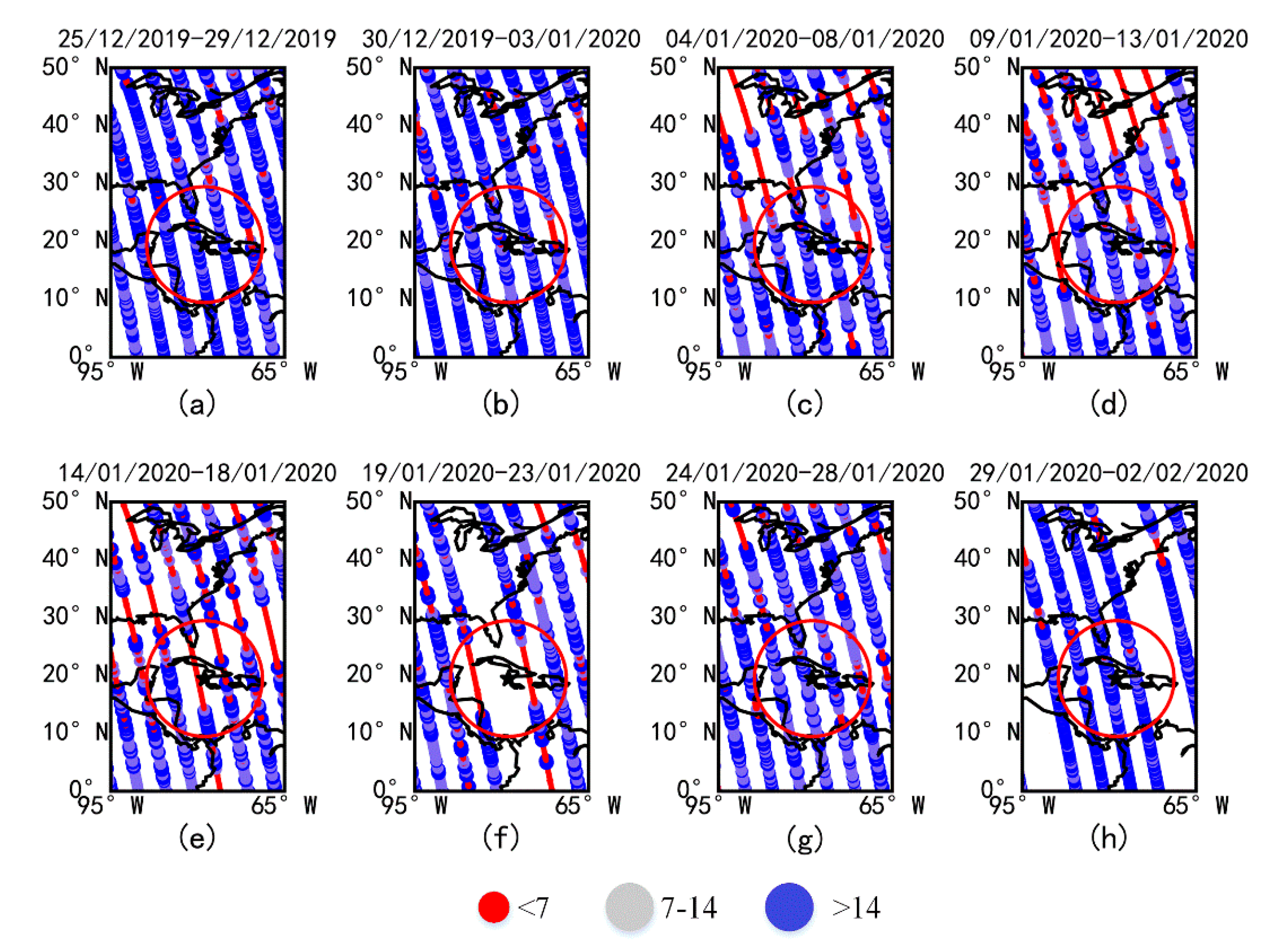
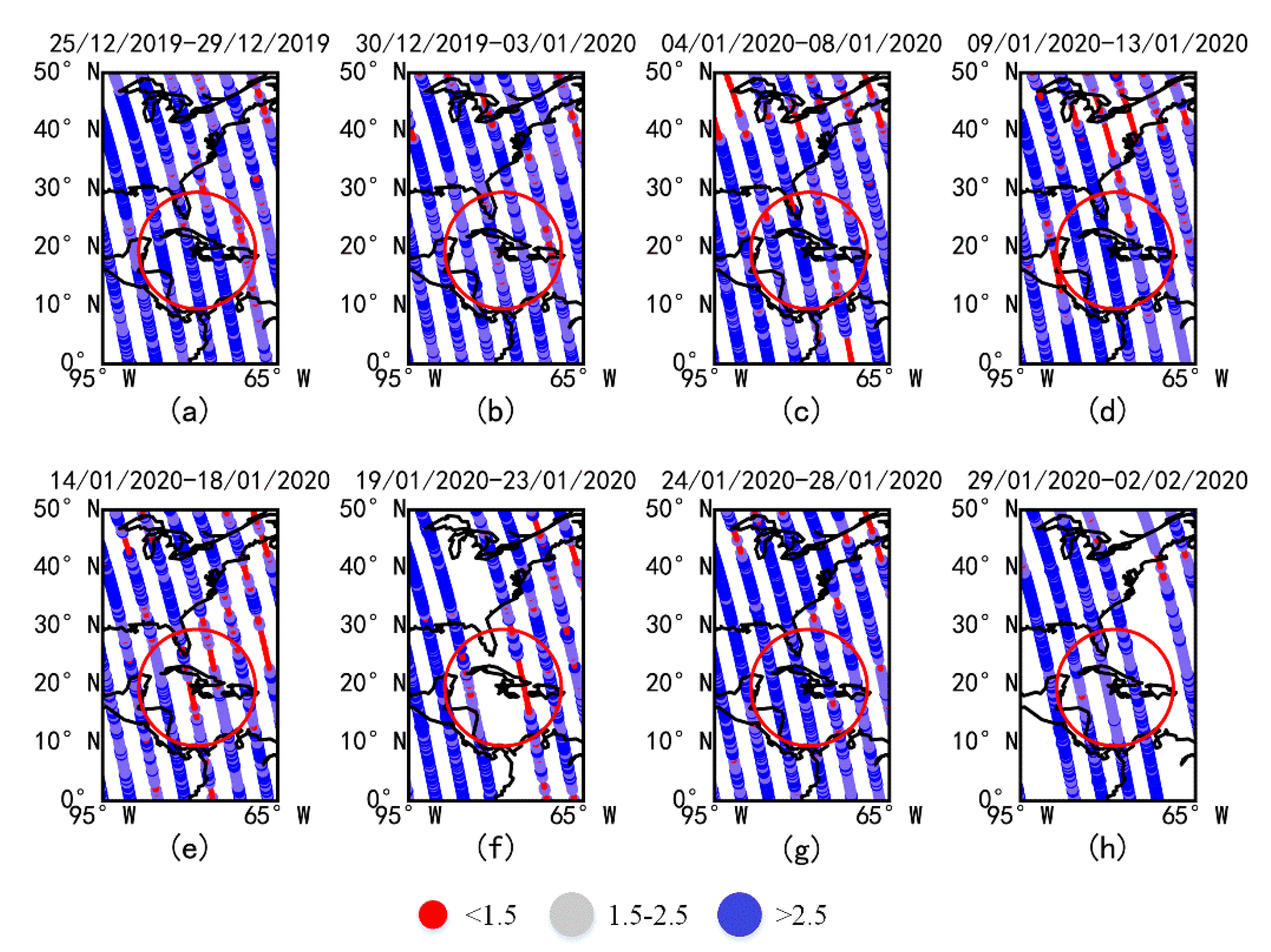
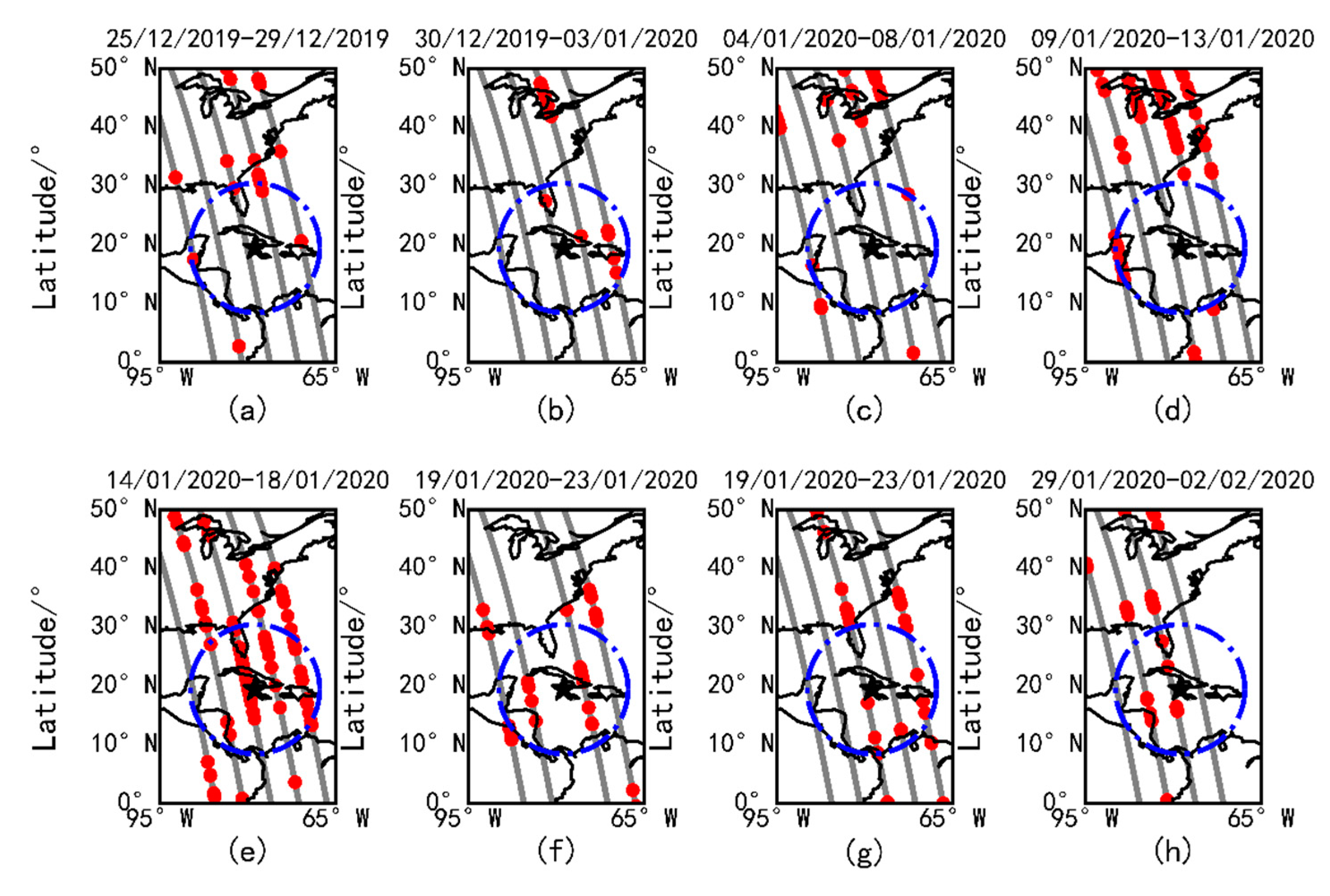
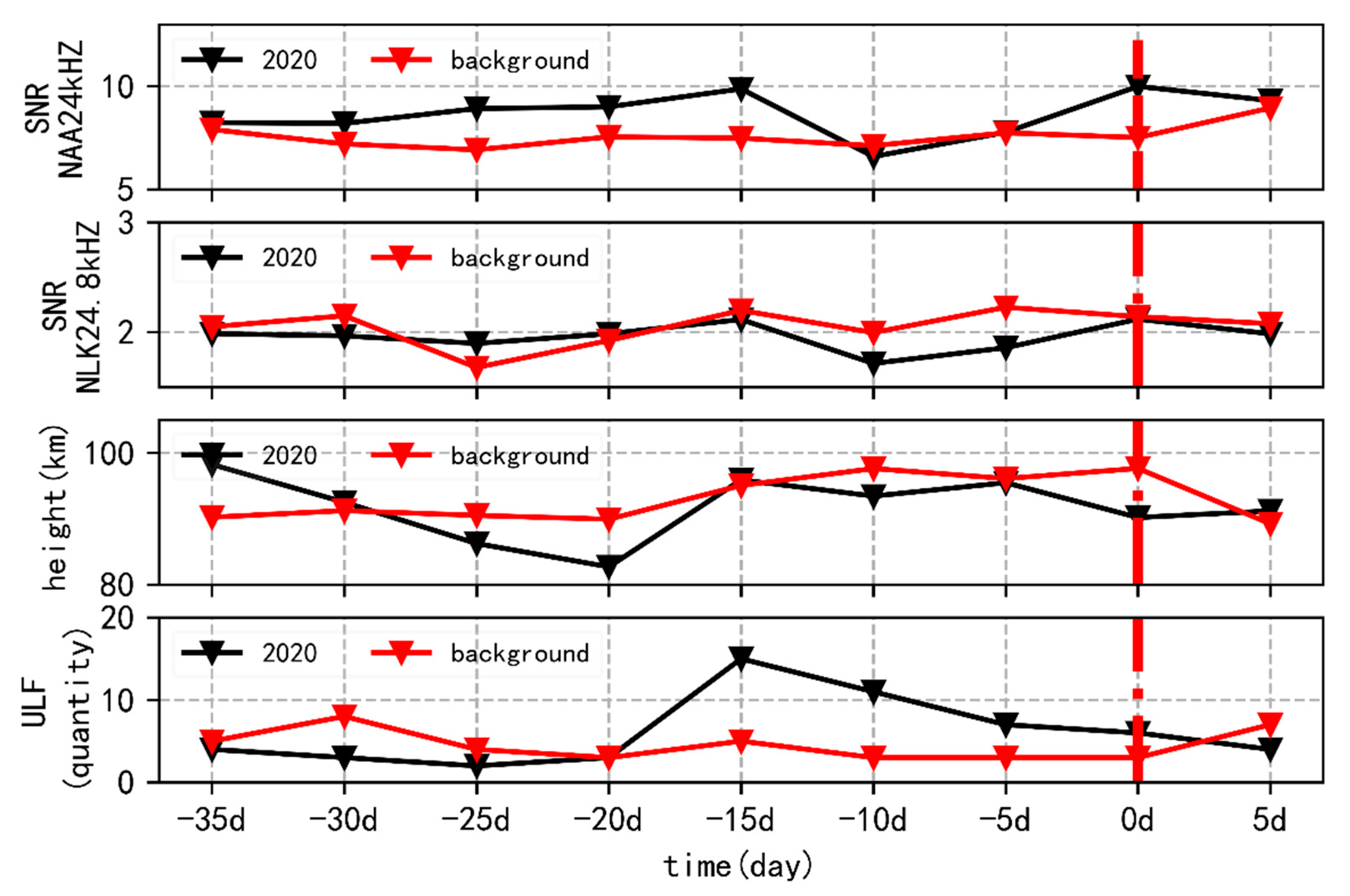
The ULF signal anomalies within the pregnant seismic area appeared widely from 15 to 10 days before the earthquake, and gradually decreased from 10 days before to 5 days after the earthquake, and most of the anomaly locations were distributed to the southeast of the epicenter. At the same time, the signal-to-noise ratio of the NAA and NLK transmitting stations also decreased substantially and recovered after the earthquake.
(2)
There was a trend of decreasing low ionospheric height during 15–10 days before the earthquake, and the decrease in the ionospheric height occurred simultaneously with the decrease in SNR.
(3)
There was a consistency in the timing of the appearance of the anomalies in the two frequency bands of ULF and VLF. Since the sources of the two bands were different and the influencing factors were different, a comprehensive analysis of the two bands, ULF and VLF, can provide a reference for accurately capturing the seismic ionospheric precursor anomalies.

Author Contributions

Conceptualization and methodology, Z.L.; Algorithm implementation, B.Y.; Data analysis and conclusion, J.H.; Writing—review and editing, H.Y.; Software and investigation, X.Y.; Visualization, F.Z.; Data curation, H.L. (Haijun Liu); Formal analysis, H.L. (Hengxin Lu). All authors have read and agreed to the published version of the manuscript.

Funding

This research was funded by a joint grant from Key Laboratory of Building Collapse Mechanism and Disaster Prevention, China Earthquake Administration (No. 2172221001), Central University basic scientific research fund (No. ZY20180121), the National Natural Science Foundation of China (No. 42104159), the APSCO Earthquake Special Project II, and ISSI-BJ2019.

Institutional Review Board Statement

Not applicable.

Informed Consent Statement

Not applicable.

Data Availability Statement

Publicly available datasets were analyzed in this study. The CSES satellite electric field data can be found at: (www.leos.ac.cn, accessed on 1 February 2022). The geomagnetic index data can be found at (http://wdc.kugi.kyoto-u.ac.jp/dstae/index.html, accessed on 1 February 2022).

Acknowledgments

This work made use of the data from the CSES mission, a project funded by the China National Space Administration (CNSA) and the China Earthquake Administration (CEA). We thank the CSES satellite team for the data (www.leos.ac.cn accessed on 1 February 2022).

Conflicts of Interest

The authors declare no conflict of interest.

References

  1. Utsu, T. A list of deadly earthquakes in the world: 1500–2000. Int. Geophys. 2002, 81, 691–717. [Google Scholar]
  2. Ding, J.H.; Shen, X.H.; Pan, W.Y.; Zhang, J.; Yu, S.R.; Li, G.; Guan, H.P. Seismo-electromagnetism precursor research progress. Chin. J. Radio Sci. 2006, 21, 791–801. [Google Scholar]
  3. He, Y.F.; Yang, D.M.; He, S.P. Preliminary Studies on Seismo-ionospheric Phenomena. Earthq. Res. China 2020, 36, 244–257. [Google Scholar]
  4. Gokhberg, M.B.; Morgounov, V.A.; Yoshino, T.; Tomizawa, I. Experimental measurement of electromagnetic emissions possibly related to earthquakes in Japan. J. Geophys. Res. 1982, 87, 7824–7828. [Google Scholar] [CrossRef]
  5. Zhang, X.M.; Shen, X.H.; Ouyang, X.Y.; Cai, J.A.; Huang, J.P.; Liu, J.; Zhao, S.F. Ionosphere VLF electric field anomalies before Wenchuan M 8 earthquake. Chin. J. Radio Sci. 2009, 24, 1024–1032. [Google Scholar]
  6. Zeren, Z.M.; Shen, X.H.; Zhang, X.M.; Cao, J.P.; Huang, J.P.; Ouyang, X.Y.; Liu, J.; Lu, B.Q. Possible Ionospheric Electromagnetic Perturbations Induced by the Ms7.1 Yushu Earthquake. Earth Moon Planets 2012, 108, 231–241. [Google Scholar]
  7. Akhoondzadeh, M. Novelty detection in time series of ULF magnetic and electric components obtained from DEMETER satellite experiments above Samoa (29 September 2009) earthquake region. Nat. Hazards Earth Syst. Sci. 2013, 13, 15–25. [Google Scholar] [CrossRef] [Green Version]
  8. Ouyang, X.Y.; Shen, X.H. A method for pre-processing ULF electric field disturbances observed by DEMETER and its case application analysis. Acta Seisynologica Sin. 2015, 37, 820–829. [Google Scholar]
  9. Ouyang, X.Y.; Parrot, M.; Bortnik, J. ULF Wave Activity Observed in the Nighttime Ionosphere Above and Some Hours Before Strong Earthquakes. J. Geophys. Res. Space Phys. 2020, 125, e2020JA028396. [Google Scholar] [CrossRef]
  10. Walker, S.N.; Kadirkamanathan, V.; Pokhotelov, O.A. Changes in the ultra-low frequency wave field during the precursor phase to the Sichuan earthquake: DEMETER observations. Ann. Geophys. 2013, 31, 1597–1603. [Google Scholar] [CrossRef] [Green Version]
  11. He, Y.F.; Yang, D.M.; Chen, H.R. Demeter satellite detected the signal-to-noise ratio change of ground VLF transmitting station signal that may be related to Wenchuan earthquake. Chin. Sci. Part D 2009, 39, 403–412. [Google Scholar]
  12. Zhao, S.; Shen, X.; Zhima, Z.; Chen, Z. The very low-frequency transmitter radio wave anomalies related to the 2010 Ms7.1 Yushu earthquake observed by the DEMETER satellite and the possible mechanism. Ann. Geophys. 2020, 38, 969–981. [Google Scholar]
  13. Hao, J.Q.; Qian, S.Q.; Gao, J.T.; Zhou, J.G.; Zhu, T. ULF electric and magnetic anomalies accompanying the cracking of rock sample. Acta Seisynologica Sin. 2003, 16, 102–111. [Google Scholar] [CrossRef]
  14. Yusof, K.A.; Abdullah, M.; Hamid, N.; Ahadi, S. Correlations between Earthquake Properties and Characteristics of Possible ULF Geomagnetic Precursor over Multiple Earthquakes. Universe 2021, 7, 20. [Google Scholar] [CrossRef]
  15. Zhang, X.M. The development in seismic application research for VLF/LF radio waves. Acta Seismol. Sin. 2021, 43, 656–673. [Google Scholar]
  16. Ma, M.J.; Lei, J.G.; Li, C.; Zong, C.; Li, S.X.; Liu, Z.; Cui, Y. Design Optimization of Zhangheng-1 Space Electric Field Detector. Chin. J. Vac. Sci. Technol. 2018, 38, 582–589. [Google Scholar]
  17. Yuan, S.G.; Zhu, X.H.; Huang, J.P. System design and key technology of China Seismo-Electromagnetic Satellite. Natl. Remote Sens. Bull. 2018, 22 (Suppl. S1), 32–38. [Google Scholar]
  18. Shen, X.H.; Zhang, X.M.; Yuan, S.G.; Wang, L.W.; Cao, J.B.; Huang, J.P.; Zhu, X.H.; Picozzo, P.; Dai, J.P. The state-of-the-art of the China Seismo-Electromagnetic Satellite mission. Sci. China Technol. Sci. 2018, 61, 634–642. [Google Scholar] [CrossRef]
  19. Molchanov, O.; Rozhnoi, A.; Solovieva, M.; Akentieva, O.; Berthelier, J.J.; Parrot, M.; Lefeuvre, F.; Biagi, P.F.; Castellana, L.; Hayakawa, M. Global diagnostics of the ionospheric perturbations related to the seismic activity using the VLF radio signals collected on the DEMETER satellite. Nat. Hazards Earth Syst. Sci. 2006, 6, 745–753. [Google Scholar] [CrossRef]
  20. Zhang, X.M.; Wang, Y.L.; Yahia, B.M.; Liu, J.; Magnes, W.; Zhou, Y.L.; Du, X.H. Multi-Experiment Observations of Ionospheric Disturbances as Precursory Effects of the Indonesian Ms6.9 Earthquake on August 05, 2018. Remote Sens. 2020, 12, 4050. [Google Scholar] [CrossRef]
  21. Toledo-Redondo, S.; Parrot, M.; Salinas, A. Variation of the first cut-off frequency of the Earth-ionosphere wave guide observed by DEMETER. J. Geophys. Res. 2012, 117, A04321. [Google Scholar]
  22. Ouyang, X.Y.; Shen, X.H. Typical interferences of ULF electric field waveform data observed by DEMETER. Seismol. Geomagn. Obs. Res. 2015, 36, 7. [Google Scholar]
  23. Savitzky, A.; Golay, M. Smoothing and Differentiation of Data by Simplified Least Squares Procedures. Anal. Chem. 1964, 36, 1627–1639. [Google Scholar] [CrossRef]
  24. Hu, Y.P.; Zeren, Z.M.; Huang, J.P.; Zhao, S.F.; Guo, F.; Wang, Q.; Shen, X.H. Algorithms and implementation of wave vector analysis tool for the electromagnetic waves recorded by the CSES satellite. Chin. J. Geophys. 2020, 63, 1751–1765. [Google Scholar]
  25. Hayakawa, M.; Hattori, K.; Ohta, K. Monitoring of ULF (Ultra-Low-Frequency) Geomagnetic Variations Associated with Earthquakes. Sensors 2007, 7, 1108–1122. [Google Scholar] [CrossRef] [Green Version]
  26. Zhang, W.; Li, Z.; Liu, H.J.; An, J.Q.; Song, Y.Y. Classification of Space Electric Field Based on Improved BP Network. Earthquake 2017, 37, 173–180. [Google Scholar]
  27. Yao, L.; Chen, H.R.; He, Y.F. Signal to noise ratio disturbance of ionospheric VLF radio signal before the 2010 Yushu MS 7.1 earthquake. Acta Seismol. Sin. 2013, 35, 390–399. [Google Scholar]
  28. Yan, R.; Wang, L.W.; Hu, Z.; Liu, D.P.; Zhang, X.G.; Zhang, Y. Ionospheric disturbances before and after strong earthquakes based on DEMETER data. Acta Seismol. Sin. 2013, 35, 498–511. [Google Scholar]
Figure 1. Lithosphere–atmosphere–ionosphere coupling mechanism.
Atmosphere 13 00934 g001
Figure 2. The power spectrum of the E-ab component of the 109,501 orbital electric field.
Atmosphere 13 00934 g002
Figure 3. The space-time diagram of the electric field SNR over the NAA transmitting station observed by the CSES (The eight subplots (ah) in Figure 3 represent a total of eight cycles from 25 December 2019, while the satellite operates every five days to 2 February 2020. The black star indicates the location of the epicenter, and the red circles indicate the seismogenic zone).
Atmosphere 13 00934 g003
Figure 4. The space–time diagram of the electric field signal-to-noise ratio over the NLK transmitting station observed by the ZH-1 satellite (The eight subplots (ah) represent a total of eight cycles from 25 December 2019, while the satellite operated every five days to 2 February 2020. The black star indicates the location of the epicenter, and the red circles indicate the seismogenic zone).
Atmosphere 13 00934 g004
Figure 5. Orbit 108,231 and its revisited orbit SNR variation graph.
Atmosphere 13 00934 g005
Figure 6. Orbit 108,381 and its revisited orbit SNR variation graph.
Atmosphere 13 00934 g006
Figure 7. The 108,231 orbital position and disturbance waveform (In subfigure (a), the black star is the epicenter position and the black curve is the satellite flight path. Subfigure (bd) depicts the small-scale residual disturbance waveforms after removing the electric field trend from the three components of the electric field ULF band).
Atmosphere 13 00934 g007
Figure 8. The 108,381 orbital position and disturbance waveform (In subfigure (a), the black star is the epicenter position and the black curve is the satellite flight path. Subfigure (bd) depicts the small-scale residual disturbance waveforms after removing the electric field trend from the three components of the electric field ULF band).
Atmosphere 13 00934 g008
Figure 9. The spatial–temporal diagram of the abnormal disturbance of the Ex component in the ULF band (the black star represents the location of the epicenter, the blue circle represents the seismogenic zone, and the red dot indicates the anomaly, In (ah), it is shown that most of the anomalies in the figure were concentrated in the area above the 40° N latitude during 35–15 days before the earthquake).
Atmosphere 13 00934 g009
Figure 10. The space–time diagram of the height of the lower ionosphere observed by the CSES (the black star indicates the epicenter location and the red circle indicates the seismogenic zone. (ah) represents the total eight cycles of satellite operation from 25 December 2019 every 5 days to 2 February 2020).
Atmosphere 13 00934 g010
Figure 11. The statistical diagram of the changes in the various parameters of the electric field in the seismogenic zone before and after the earthquake.
Atmosphere 13 00934 g011
Figure 12. Change in the space weather index from 15 December 2019 to 13 February 2020.
Atmosphere 13 00934 g012
Table 1. Data products under different working modes.
Working ModeDC-ULF (0~16 Hz)ELF (6 Hz~2.2 kHz)VLF (1.8 kHz~20 kHz)HF (18 Khz~3.5 MHz)
BURSTwaveformswaveformswaveforms
SURVEYwaveformswaveformsspectraspectra
Table 2. The list of artificial source transmitting stations.
CodeLongitude [°]Latitude [°]Frequency [Hz]Power [kW]
NAA−67.3044.6524,0001000
NAU−67.1018.2340,750100
NLK−121.9048.2024,800192
NML−98.2046.2125,200-
Publisher’s Note: MDPI stays neutral with regard to jurisdictional claims in published maps and institutional affiliations.

