1. Introduction
Great efforts have been made recently in the field of space weather—the set of space factors that influence technical, industrial, and economic human activities. Space weather research, forecasting, and real-time diagnostics become the most urgent problems of modern near-space physics [
1,
2,
3,
4,
5]. Space weather includes the complex chain of interactions between solar emissions (solar irradiation and solar plasma) and Earth’s magnetic field, while the ionosphere plays an important role in its diagnostics as a primary indicator of solar-terrestrial interaction [
6].
At high latitudes, there are two main sources of atmospheric gas ionization by the extreme ultraviolet (EUV) solar radiation and the electron precipitation from the magnetosphere. Magnetospheric 1–10 keV electrons release their energy in the ionosphere E layer at 90–140 km altitudes, playing an important role in chemical, optical, and electrodynamic processes [
7]. Due to precipitation of magnetospheric electrons, the Hall and Pedersen conductivities reach their maximum at these altitudes leading to development of horizontal ionospheric electrojets which close magnetospheric field-aligned currents [
8,
9].
Dynamics of the electric currents in the E layer are responsible for various ground magnetic disturbances [
10,
11,
12]. Ionospheric currents, associated with strong magnetospheric perturbations, can induce the harmful parasitic electric currents in long technological structures on the Earth’s surface—communication lines, electrical power systems, and pipelines [
3,
13,
14]. Additionally, the unsteady dynamics of sporadic particle precipitation in the E layer can lead to a rapid change in the radio wave propagation conditions [
15], complicating the diagnostics and forecasting of high frequency radio paths.
Many theoretical problems and practical applications related to the high-latitude ionosphere require complex analysis of regular ground and spacecraft measurements in combination with the numerical modeling of the geophysical processes. The Auroral Ionosphere Model (AIM-E) [
16] is specially designed for the high-latitude E region of the ionosphere and takes into account the solar EUV radiation flux and the global spatial distribution of precipitating magnetospheric electrons. Both ionization sources can be set using actual spacecraft measurements or/and empirical models. In the case of electron precipitation input, the spacecraft-based measurements provide a high accuracy of ionospheric solution along the spacecraft trajectory, while the empirical model of precipitating particle distribution can be used for a climatological modeling to describe the large-scale ionosphere dynamics in the auroral zone [
16]. AIM-E provides the chemical composition of the high-latitude ionosphere in the altitude range from 90 to 140 km. The model calculates concentrations of 10 ionospheric components: three small neutral components
NO,
N(4S),
N(2D), and 7 ions
N+,
N2+,
NO+,
O2+,
O+(4S),
O+(2D),
O+(2P), taking into account their interactions in 39 chemical reactions.
One of the main challenges in modeling of auroral ionosphere is to correctly determine the spatial distribution of particle precipitation in the course of geomagnetic storms and substorms. The AIM-E model uses the OVATION-Prime empirical model [
17] to emulate the magnetospheric precipitation source. The OVATION-Prime model allows to estimate the intensity of four types of auroral precipitation: monoenergetic, broadband (“Alfvenic” or wave aurora), diffuse electron precipitation, and ion precipitation poleward from the 50° magnetic latitude [
18]. The model application is limited by Kp = 5+ geomagnetic activity level. The OVATION-Prime is a useful tool and widely used for different space weather services (e.g., prediction of visible aurora [
19]).
OVATION-Prime was constructed using DMSP spacecraft measurements of particle precipitation during two solar activity cycles and parameterized by the coupling function built on OMNI2 solar wind hourly average data [
20], which are based on the spacecraft measurements far upstream of the Earth’s bow shock, mainly in the Lagrange point L1 (at the distance of ~1.5 million km from the Earth).
Accuracy of OMNI IMF-based parameterization suffer from two main reasons: (1) solar wind parameters measured at the Lagrange point L1 are not always geoeffective (not the same at the L1 and the Earth orbit), and in 20% of cases do not interact with the magnetosphere at all [
21,
22]; (2) spatial distribution and energy spectrum of precipitating particles significantly depend on the internal magnetospheric processes, in other words, under similar solar wind conditions, magnetospheric state and hence, magnetosphere–ionosphere interaction may differ dramatically depending on previous magnetospheric dynamics [
23,
24].
In order to improve the accuracy of AIM-E model when simulating highly variable periods during geomagnetic storms and substorms, we use OVATION-Prime model with modified parameterization, where the solar wind-based Newell’s coupling function (
N) is changed for the ground-based Polar Cap (PC) index, responding in the real-time to the solar wind energy input into the magnetosphere [
25]. Hereinafter, we will use the designations OVATION-Prime (PC) and AIM-E (PC) to reflect the modification of the models switching to the PC input.
In this study, we simulate the high-latitude ionosphere in the E region during disturbed geomagnetic conditions using the AIM-E model with PC index as a control parameter for the electron precipitation source. To validate the new parameterization, we analyze the simulation results together with UHF EISCAT (Tromso, Norway) radar measurements and ionosonde data in the Arctic zone.
2. Materials and Methods
The AIM-E model allows us to estimate the concentration of the small neutral components, ions, and electrons in the whole auroral ionosphere E region [
16]. The model is capable of reproducing the ionospheric response to the geomagnetic storms and substorms with sufficient accuracy, and can be used to describe the dynamics of chemical content in the auroral oval during disturbed periods.
The 4th order implicit numerical scheme with a variable integration step is used to solve the stiff differential continuity equations system for 10 ionospheric species. This method significantly reduces the computational costs and, at the same time, ensures a sufficient numerical solution accuracy. High performance of the AIM-E model allows to calculate, in real-time, the entire auroral zone composition covering the altitude range of 90–140 km in real-time, taking into account different levels of solar ultraviolet radiation [
26] and for high variability of electron precipitation in auroral zone [
16].
The OVATION-Prime model is integrated into AIM-E to provide the spatial distribution of electron precipitation parameters at high latitudes (MLAT = 50°–90°) on a discrete grid (MLT × MLAT = 0.25 h × 0.25°). The model is based on the DMSP particle data for two solar cycles and normalized on the OMNI solar wind (SW) parameters in the following form [
27]:
where
v is the SW speed;
BT is the interplanetary magnetic field (IMF) tangential component, B
T = ;
θ is the IMF clock angle, θ = arctan (By/Bz).
The geomagnetic index PC was put forward as a characteristic of the polar cap magnetic activity [
28]. The index is calculated online by data of ground-based magnetic observations at stations Vostok in Antarctica (PCS index) and Thule in Greenland (PCN index). The index was approved by the International Association of Geomagnetism and Aeronomy (IAGA) as an indicator of the solar wind energy input into the Earth’s magnetosphere in the course of the solar wind–magnetosphere coupling (Resolution of XXII IAGA Assembly, 2013).
The PC index is normalized to the solar wind electric field E
KL [
29,
30] being calculated according to [
31]:
EKL = v BT sin2(
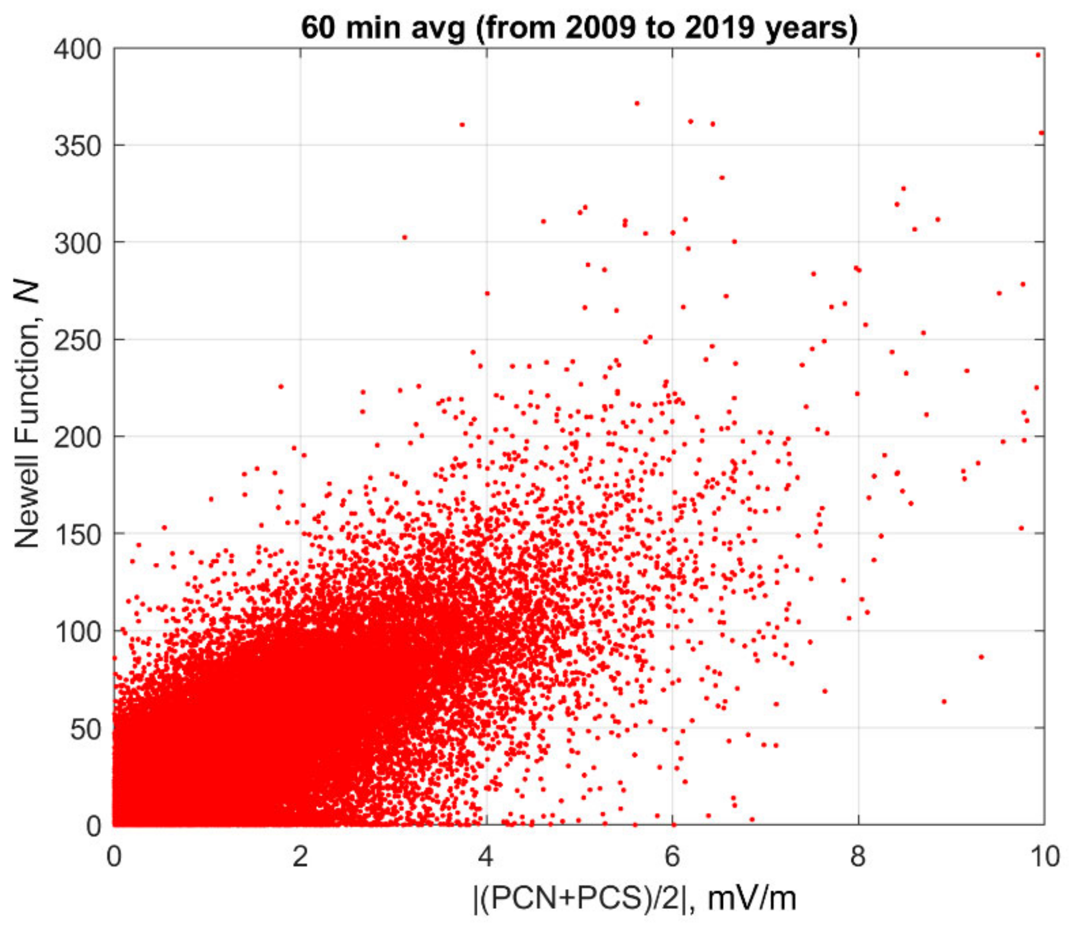
θ/2). Having similar solar wind normalization, the Newel’s
N coupling function and PC index turn out to be closely related, with discrepancy due to
N distortion on the way from solar wind to magnetosphere. The correlation coefficient between the hourly averages of the Newell’s function and PC index over a ten-year period is 0.76 (
Figure 1). The comparative data analysis of PC index and the Newell’s coupling function with the integrated auroral power of particle precipitation obtained from the Polar satellite shows that the PC index correlates with the magnitude of auroral power much better (the correlation coefficient R
PC∼0.76−0.87, depending on the time delay) than the Newell’s coupling function (R
N∼0.46−0.82), and especially in the real-time mode R
PC = 0.76 versus R
N = 0.46 [
32]. Furthermore, it was shown that PC index has a high correlation with basic indices of magnetospheric disturbances AL and Dst [
24,
25,
33].
Based on these results, it becomes possible to use PC index instead of Newell’s function in the OVATION-Prime precipitation model. The modified OVATION-Prime with PC application was already successfully used to study processes in the Earth’s atmosphere in [
34], where the multi-regression formula was taken to switch from
N to PC index:
where
ki are regression coefficients;
PC is PC index averaged between the northern and southern hemispheres, and
∆PC5 and
∆PC10 are the changes of PC magnitude within the 5 and 10 min intervals respectively.
Here, we use the modified OVATION-Prime (PC) as a source of electron precipitation to improve the AIM-E model accuracy when simulating disturbed periods during geomagnetic storms and substorms.
3. Results
3.1. Comparison of the AIM-E Results with EISCAT UHF Measurements
Studying the dynamics of the auroral ionosphere during periods of storms and substorms, it is necessary to have a control parameter that can describe rapidly changing conditions in the inner magnetosphere. The use of minute values of the PC index as an input parameter of the high-latitude E region ionosphere model makes it possible to take into account the fast variations of electron precipitation flux during the periods with high geomagnetic activity.
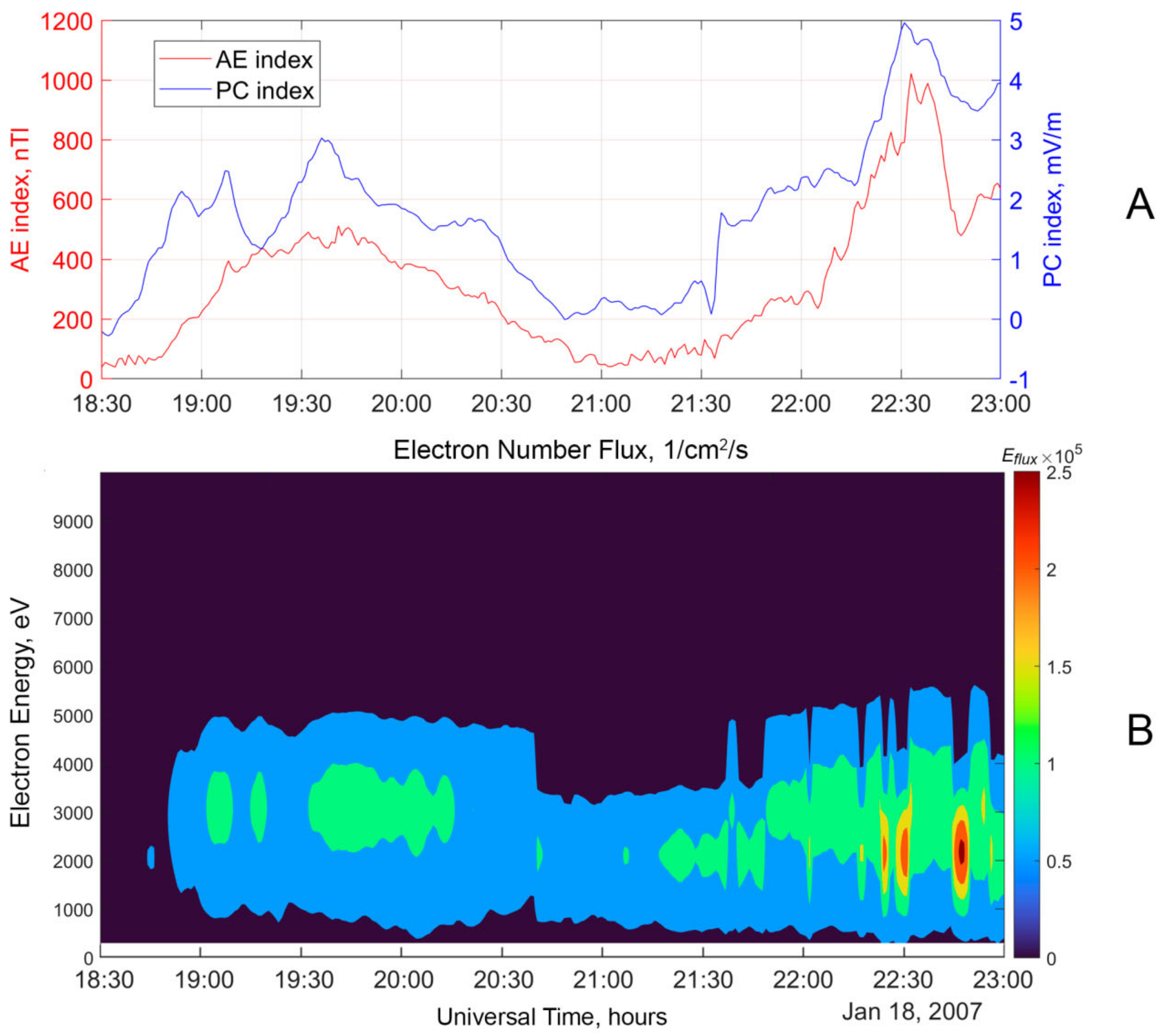
To validate the AIM-E (PC) model we compared the simulated electron density with the incoherent scattering radar data during disturbed geomagnetic conditions on 18 January 2007, 18:30–23:00 UT, including two substorms (18:00–21:00, AE index increase to 450 nT; 21:00–23:30, AE index maximum 1000 nT (
Figure 2A, red)). Variation of the geomagnetic index PC (an average between the northern (PCN) and southern (PCS) indices) for this event is shown in
Figure 2A (blue).
The energy spectra of precipitating electrons were reconstructed from the OVATION-Prime (PC) number flux and average energy outputs for: (1) diffuse electrons, assuming the Maxwellian distribution of the spectrum and (2) monoenergetic electron beams, using the normal distribution with a dispersion of a given value equal to half the difference between the channels adjacent to the channel of maximum energy. Time variation of the reconstructed spectrum over the EISCAT radar location, covering energies from 300 eV to 10 keV and used in AIM-E simulation, is shown in
Figure 2B.
According to OVATION (PC) simulation, the electron precipitation intensifies during both substorms. For the second substorm, we observe particle flux peaks 2.5 times larger than for the weaker first substorm.
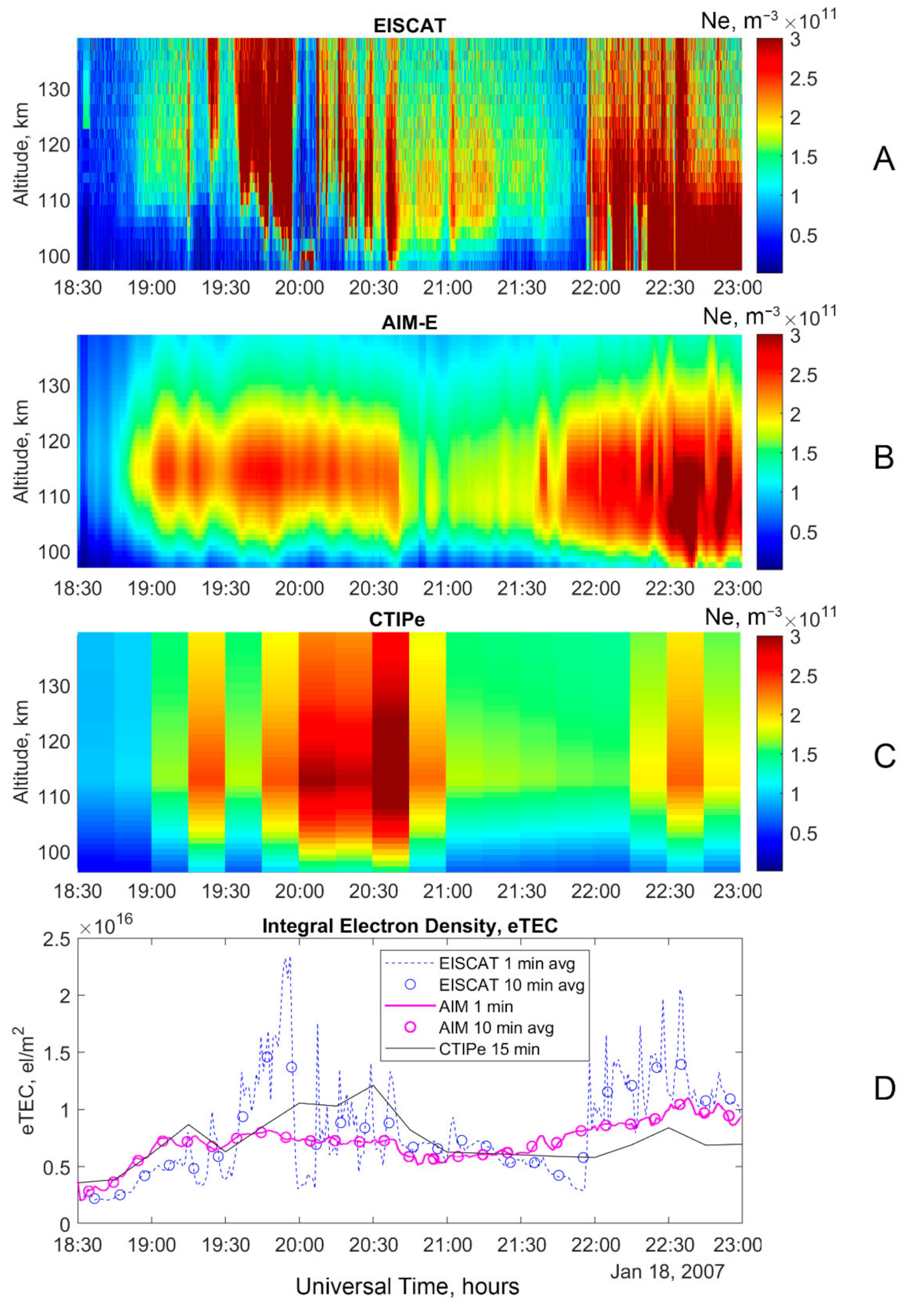
The AIM-E (PC) calculations were done at the location point of the incoherent scatter radar EISCAT, Tromso (69°35′ N, 19°13′ E), in the altitude range 96–140 km with 1 km altitude step and 1 min time resolution (
Figure 3B). It is clear that the peaks of the simulated electron concentration are synchronized with the intensifications of electron precipitation within the 1–5 keV energy range. This part of the spectrum has the greatest influence on the E layer ionization.
Figure 3A shows the evolution of electron density in the 96–140 km altitude range measured by the UHF EISCAT incoherent scatter radar [
35]. The radar operated under the ARC1 sounding program: altitude range: 96–422 km; altitude step: 0.9 km; time resolution: 0.44 s; the antenna is directed towards the magnetic zenith.
It is remarkable that the time intervals of enhanced electron concentration observed by the radar and obtained using AIM-E (PC) coincide well. In both cases (real measurements and model), the electron concentration increases from background values (1 × 10¹¹ m–3) to about 3 × 10¹¹ m–3 during substorms.
The maximum of the simulated E layer is pronounced and located approximately around 110–115 km altitude, while the radar data shows a wider spread of enhanced electron concentration by altitude. The difference in the Ne altitude distribution can be explained by the difference in the shape of the real and reconstructed spectra of precipitated electrons: AIM-E simulation considers both diffuse and monoenergetic electron precipitation flux but the real electron spectrum shape is poorly predictable and can make a significant contribution to altitudinal distribution of ionospheric ionization.
In order to compare the model and incoherent scatter radar data, we calculate the time variation of an integral electron content between 96 and 140 km altitude, which can be treated as a partial TEC confined in the E layer (hereinafter, eTEC) (
Figure 3D). The correlation coefficient between the AIM-E (PC) and EISCAT minute values of the eTEC is R
1min = 0.63. Using a 10-minute averaging, the correlation coefficient rises up to R
10min = 0.78, which we consider as a good result for local calculations in the auroral zone during active substorm interval.
Results in
Figure 3D show that modeling of the ionospheric content in the auroral region considering diffuse and monoenergetic electron precipitation by OVATION-Prime (PC), makes it possible to estimate the “background” E layer electron content, while the fine structure of the disturbed oval, measured by the EISCAT radar (
Figure 3D), cannot be reproduced in the “climatological” mode. Moreover, the absence of transport processes in the model may be responsible for systematic underestimation of the electron density above 110 km.
3.2. Comparison of the AIM-E Results with CTIPe Model
To understand the capabilities of the AIM-E (PC) in comparison with other high-latitude ionosphere models, we performed the simulation of the event described in
Section 3.1 (18 January 2007 18:30–23:00 UT), using an advanced ionospheric CTIPe model which is available at the Community Coordinated Modeling Center (CCMC) [
36].
The Coupled Thermosphere Ionosphere Plasmasphere Electrodynamics Model (CTIPe) [
37] evaluates the concentration of electrons, neutrals
O,
O2,
N2, and ions
H+,
O+ in the altitude range from 140 to 2000 km, and additional
O2+,
N+,
N2+ ions below 500 km. CTIPe consists of four separate blocks: (1) Global thermosphere model; (2) High-latitude ionosphere model; (3) Ionosphere/Plasmasphere model of middle and low latitudes; (4) Electrodynamic calculation of the global dynamo-electric field.
The input CTIPe parameters are the SW density, velocity, and IMF components from the DSCOVR or ACE satellites [
38] for real-time mode or OMNI data for simulation of historical events. The ionosphere electric fields are set according to the Weimer electrodynamics model [
39]. Moreover, the input parameter of the model is a radio flux at 10.7 cm. The CCMC version of the model has a 15-minute time resolution.
Figure 3C shows the evolution of the altitude profile of electron concentration on 18 January 2007, 18:30–23:00 UT simulated by the CTIPe model.
The CTIPe model, with a 15-minute SW input data, as well as the AIM-E (PC) model, qualitatively and quantitatively describe ionospheric dynamics at the EISCAT location quite well. Both models almost synchronously demonstrate an increase in the electron concentration during the substorm periods. The CTIPe model better reproduces the vertical structure of E region electron density for the first substorm. However, for the second disturbed interval (after 22:00 UT), the AIM-E (PC) model better agrees with the EISCAT data. This is also confirmed by the integral electron density variation shown in
Figure 3D. The CTIPe’s eTEC variation is in better agreement with the radar data for the first substorm and gives underestimated values for the second one. However, we would like to note that for the first substorm, the maximum electron density according to the CTIPe model is observed from 20:00 to 20:45, while the EISCAT data and AIM-E model shows the Ne increase in the time interval from 19:30 to 20:00. The better timing of AIM-E model is provided by using the ground PC index (instead of coupling functions based on solar wind measurements), which immediately responds to energy input into the ionosphere.
3.3. Application of AIM-E (PC) for Monitoring of Sporadic E layers
Sporadic E layers on the vertical sounding (VS) ionograms appear as a signal reflection at frequencies significantly higher than the critical frequency of the regular E layer (f
OE) [
40]. The maximum reflection frequency of such layers can reach 10–12 MHz, shielding the overlying ionosphere from the radio waves emitted from below. Sporadic layers are found all over the globe and they are traditionally divided into three classes: equatorial or low-latitude, mid-latitude, and auroral or high-latitude. Sporadic layers may also differ in their formation mechanisms. Knowing the layer type can help to interpret the processes of magnetosphere–ionosphere interaction and neutral atmosphere dynamics.
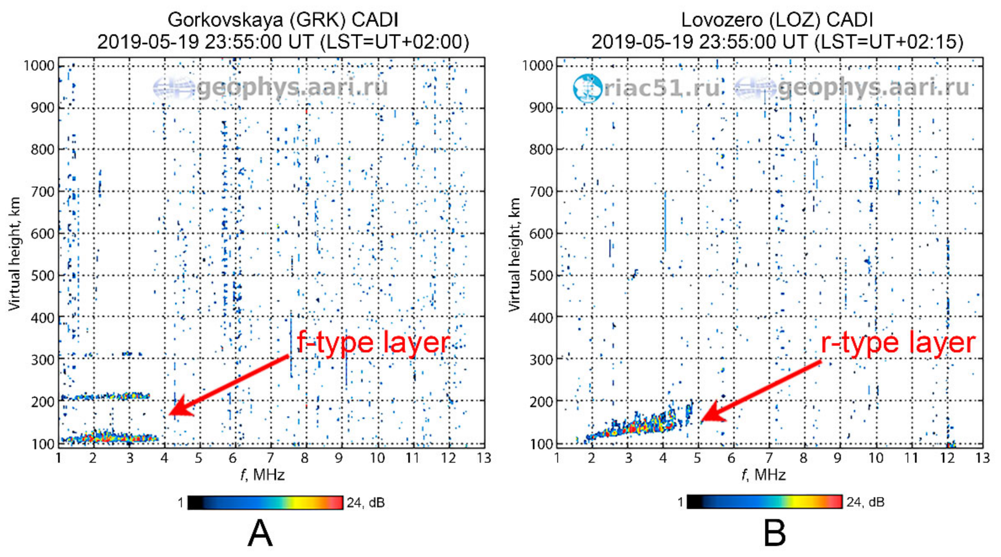
Depending on the VS signal reflection shape, several types of sporadic layers are distinguished:
f—flat layer—does not show an increase in height with frequency;
r—thick layer—a reflecting signal track of this type has an increase of the effective height at the high-frequency edge, like the regular E layer track;
a—auroral layer—has a well-pronounced flat or gradually increasing lower edge, with delamination and diffuse reflection above it.
Appearance of a thick and auroral sporadic layer (type r and a) is associated with the electron precipitation. Just this physical mechanism of ionization was incorporated in the AIM-E model.
Formation of sporadic flat layers (type f) at mid-latitudes is explained by the “wind-shear” effect: neutral wind leads to changes in horizontal drift and results in the vertical ions movement, which leads, in the presence of a sufficient amount of metal ions (Mg
+, Fe
+, etc.), to the formation of thin ionization layers [
41]. To explain formation of flat layers at high latitudes, a combination of tidal wind-shear and electric field drift theories is usually applied [
42,
43]. At the same time, the signs of metal ions’ presence at high-latitude flat layers were also detected by data of the UHF EISCAT Tromso [
44,
45], and using the Sondrestrom IS [
46] radar measurements.
The AIM-E model does not consider mechanisms associated with the ion transport. However, the model can be successfully used to describe the sporadic layer, which is most often formed in the auroral zone as a thick r-type layer. To demonstrate the ability of the AIM-E model to predict the sporadic layers’ formation, we performed the simulation of an isolated substorm that occurred between 23:00 UT on 19 May and 04:00 UT on 20 May 2019, and compared simulation results with VS measurements.
The moderately disturbed geomagnetic conditions have been observed during the considered period: AE index increased up to 1000 nT, and the planetary geomagnetic index Kp did not exceed 3+. This is an important note for the OVATION-Prime calculations since the accuracy of the precipitation model degrades at Kp > 5 [
17].
Ionosonde Data
The Ionosonde data for this study was provided by Geophysical Data Center of Arctic and Antarctic Research Institute [
47]. We used the critical frequency values (f
OE) obtained from ionograms for each 15-minute sounding session. Vertical sounding (VS) data were received from Gorkovskaya (GRK) and Lovozero (LOZ) stations; oblique sounding (OS) data were taken at the central point of their radio path Gorkovskaya–Lovozero (GRK–LOZ). Geographic and corrected geomagnetic coordinates of stations are presented in
Table 1 and their location is shown in the accompanying map. During the interval of interest, we obtained 29 and 9 f
OE and f
OEs values from the VS ionograms, and 18 f
OE values using the oblique sounding method which is not applicable for the layer-type determination.
According to these measurements, the presence of both flat (f-type) and thick (r-type) sporadic layers were recorded during the substorm. Examples of VS ionograms on 19 May 2019 at 23:55 UT show the presence of f-type sporadic layer at Gorkovskaya (
Figure 4A), and r-type sporadic layer at Lovozero station (
Figure 4B).
The AIM-E (PC) vertical profiles of the electron concentration in the VS/OS observation points were calculated in the altitude range of 90–140 km with 1 km step size and 1 min time resolution. For each profile, we calculate the E layer critical frequency as:
where
fOE is the sounding critical frequency (MHz) and
Nemax is the maximum value of electron concentration in the vertical profile (m
–3).
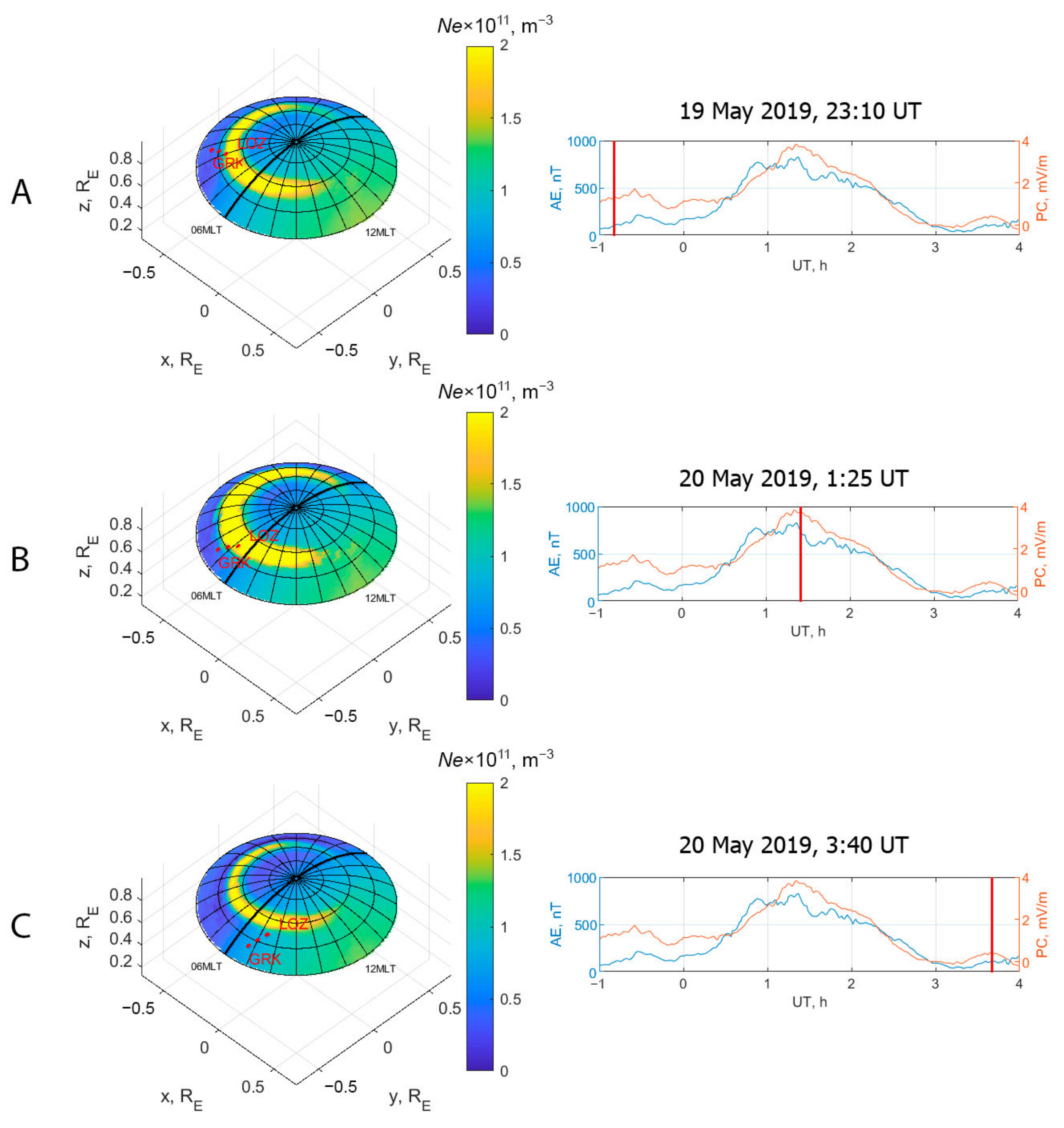
Figure 5 shows the maps of the
Nemax distribution for three time moments: A—23:10 UT (before the substorm); B—1:25 UT (substorm expansion); C—3:40 UT (after the substorm). Geomagnetic activity during this event is shown by the AE and PC indices in the right column of
Figure 5 (red and blue lines respectively). The spatial dynamics of
Nemax during the entire substorm interval (between 23:00 UT on 19 May and 04:00 UT on 20 May 2019) is shown as a movie attached in the
Supplementary Materials (Movie S1).
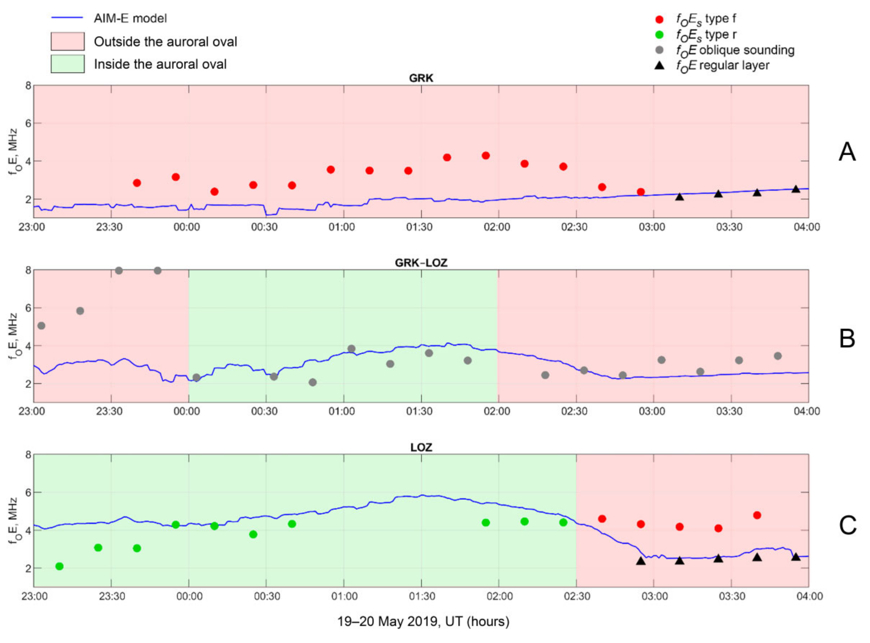
According to the AIM-E model, the GRK–LOZ central observation point was inside the auroral oval from 0:00 to 2:00 UT; LOZ—from 23:00 to 2:30 UT (
Figure 6B,C, marked with green background). For the entire observation period, the subauroral station GRK was located outside the active precipitation zone (
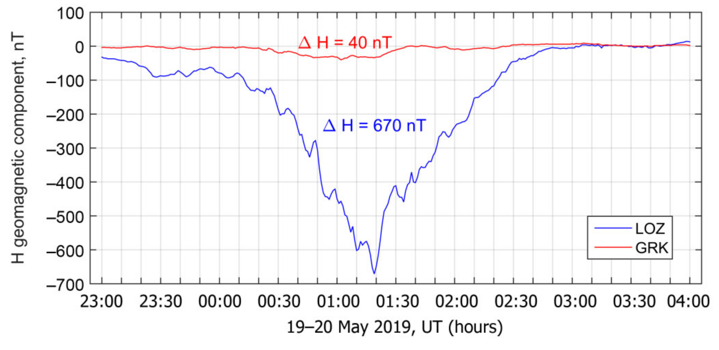
Figure 6A, marked with red background). This disposition is also confirmed by the data of magnetic observations at the stations GRK and LOZ (
Figure 7). The geomagnetic disturbance in the H-component at GRK stays quiet (<40 nT) during the entire period. At the same time, a moderate but expressed magnetic bay with 670 nT peak value is observed at LOZ station, indirectly confirming its location within an active precipitation zone.
The OS and VS comparison with model results is shown in
Figure 6A; sporadic flat layer (type f, red circles in
Figure 6) was observed during the entire interval (partly at GRK and partly at LOZ station), but the measured f
OEs values clearly exceed the simulated ones. For the period until 2:30 UT, the LOZ station (
Figure 6C) was within the auroral oval and observed the thick (type r) sporadic layer critical frequencies which are in a good agreement with the AIM-E (PC) results. Beginning from 2:30, the LOZ ionograms allow to determine the regular layer and sporadic f-type layer simultaneously. Again, the model failed to predict the f-type layer, but the regular layer fits perfectly to observations (
Figure 6A, 3:00–4:00 UT).
Although it is impossible to determine the type of layer using OS ionograms (
Figure 6B), we can still make some suggestions for the GRK–LOZ central point. Until midnight (outside the oval), the OS critical frequency values significantly exceed the simulation results. Here we can assume the formation of a flat sporadic layer which is not reproducible in AIM-E simulations. Further, from 0:00 to 2:00, when the OS central point was inside the auroral oval, the same r-type layer was observed simultaneously with the LOZ station. At the end of the observation interval, from 2:00 to 4:00, it is natural to assume the presence of the regular layer, observed simultaneously at both GRK and LOZ stations.
Since it is widely accepted that transport effects are negligible for the ionosphere in the high-latitude E region [
48] the AIM-E model in current implementation does not take into account the particle drift effects. However, as analysis shows, for a detailed description of the formation of sporadic layers, it is necessary to take into account the processes of charged particle transport caused by neutral winds and electric drift. Moreover, it can be important to include the metal ions to the high-latitude E layer model [
49,
50]. This is foreseen in our plans for the further development of the AIM-E model.
4. Conclusions
The E Region Auroral Ionosphere Model (AIM-E) is a useful scientific and operational numerical tool for various geophysical applications. It can be used to reconstruct the large-scale dynamics of the auroral ionosphere with sufficient accuracy during disturbed geomagnetic periods. The modified AIM-E model applying the Polar Cap index as an input parameter, becomes the unique high-latitude ionosphere model which operates only with the ground-based data.
The first advantage of this approach is that we can consider the actual solar wind energy input based on the magnetic observations in the polar caps. This factor provides more accurate timing for the auroral ionosphere dynamics, which is especially important during geomagnetic storms and substorms.
The second advantage is that AIM-E (PC) is independent from the space observations so the model can operate even when the solar wind data are unavailable.
While describing the high-latitude ionosphere, the AIM-E (PC) model can be successfully used to determine the base level of the electron concentration at auroral latitudes. At this point, the results of the AIM-E (PC) simulation for the disturbed geomagnetic conditions demonstrate a reasonable agreement with ground-based ionospheric observations, including the EISCAT radar data and the vertical sounding data. Based on the empirical precipitation model (not using in situ spacecraft measurements), the AIM-E (PC) model well reproduces the background value of the electron content calculated in vertical column (90–140 km) and critical frequency of sporadic E layer (fOE) formed by precipitating electrons. The model can be successfully used to describe the large-scale dynamics of the auroral oval during disturbed periods.
The model can be applied to monitor both regular and sporadic precipitation-originated layers in the E region in a real-time and in the entire high-latitude ionosphere, including the auroral and subauroral zones. It is essential for predicting the conditions of radio wave propagation and the space weather nowcasting.


