A Statistical Analysis of Sporadic-E Characteristics Associated with GNSS Radio Occultation Phase and Amplitude Scintillations

Abstract

Statistical GNSS-RO measurements of phase and amplitude scintillation are analyzed at the mid-latitudes in the local summer for a 100 km altitude. These conditions are known to contain frequent sporadic-E, and the S${}_4$-${\sigma }_{\varphi }$ trends provide insight into the statistical distributions of the sporadic-E parameters. Joint two-dimensional S${}_4$-${\sigma }_{\varphi }$ histograms are presented, showing roughly linear trends until the S${}_4$ saturates near 0.8. To interpret the measurements and understand the sporadic-E contributions, 10,000 simulations of RO signals perturbed by sporadic-E layers are performed using length, intensity, and vertical thickness distributions from previous studies, with the assumption that the sporadic-E layer acts as a Gaussian lens. Many of the key trends observed in the measurement histograms are present in the simulations, providing a key for understanding the complex mapping between layer characteristics and impacts on the GNSS-RO signals. Additionally, the inclusion of Kolmogorov turbulence and a diffusion-limited threshold on the lens strength/(vertical thickness)${}^2$ ratio helps to make the layers more physically realistic and improves agreement with the observations.

1. Introduction

With modern day society’s strong reliance on GNSS for both navigation and timing, scintillation caused by ionospheric irregularities can induce loss of lock and increase navigation errors [1,2,3], thereby seriously impacting our technological infrastructure [4]. While ground-based GNSS receivers are most severely perturbed by equatorial plasma bubbles (EPBs) [5], sporadic-E (E${}_s$) is the leading cause of spaced-based GNSS cycle slips from an E-region ionospheric irregularity [6]. Sporadic-E manifests as enhanced ion layers caused by metallic ion convergence through neutral wind shears [7,8]. The sporadic-E layers are typically referred to as “clouds” because of their non-uniform, patchy nature. The E${}_s$ impact on radio wave propagation, in terms of over-the-horizon radar and global positioning system (GPS) timing for low Earth orbit (LEO) satellites, relies not only on the presence of sporadic-E but also on the specific characteristics.

Many methods for measuring or characterizing E${}_s$ have been proposed and implemented in previous studies, including incoherent scatter radars (ISRs) [9], ionosondes [10,11,12,13,14,15], and global navigation satellite system (GNSS) radio occultation (RO) [16,17]. While ISR measurements provide detailed information on the sporadic-E layers, the limited number of global sites and measurement cadence inhibit statistical analyses of E${}_s$ layers. Ionosondes provide direct measurements of sporadic-E intensity and height, but layer characteristics such as length or vertical thickness are difficult to obtain, given the spatial separation between ground sites and the vertical orientation of the measurements.

GNSS-RO has shown promise for monitoring [17,18,19] and characterizing [20,21,22] sporadic-E layers due to the relatively thin vertical structures that significantly perturb GNSS signals as they propagate horizontally across the ionosphere to a LEO satellite. This geometry allows for characterization of sporadic-E using GNSS-RO, while the relatively long horizontal lengths require exceptionally strong layers to observe in ground-based GNSS sensors [23]. While the large number of global GNSS-RO measurements with high spatiotemporal resolutions (see [24] for more detail) provides a unique method for characterizing global E${}_s$ characteristics and patterns, the amplitude and phase measurements are often difficult to interpret because of the integrated nature of the observations [25,26].

To help with the interpretation of GNSS-RO observations of sporadic-E, multiple-phase screen simulations of the signal perturbation have guided the mapping of sporadic-E characteristics to amplitude perturbations [17,20,27]. As shown in the simulations, the magnitude of amplitude fluctuations in terms of a scintillation index such as S${}_4$ are strong functions of the sporadic-E layer’s vertical thickness, length, intensity (foEs), and orientation. While the vertical thickness can be estimated from GNSS-RO observations [20], the length and intensity are both unknown from GNSS-RO measurements alone, which makes the intensity estimates uncertain [25]. However, simulations can help in our understanding of the complex mapping between the layer properties and observed GNSS-RO signals.

Here, we provide a statistical view of GNSS-RO scintillation observations in terms of the phase standard deviation ${\sigma }_{\varphi }$ and amplitude scintillation index S${}_4$ over a month-long period over the mid-latitudes during the local summer at an E-layer altitude of 100 km. Then, to help interpret the results, we simulate GNSS-RO signals after traversing sporadic-E layers in an attempt to reproduce the measured data. Ultimately, we are able to reproduce many of the unique trends from the observations using standard E${}_s$ distributions for length, intensity, and vertical thickness with the assumption that the E${}_s$ layer acts as a Gaussian lens. Finally, inclusion of turbulence to the idealized Gaussian lens helps to improve the agreement between the simulation and measurements.

2. GNSS-RO Scintillation Measurements

2.1. S${}_4$ and ${\sigma }_{\varphi }$ Calculations

In this study, the S${}_4$ index is calculated from the Constellation Observing System for Meteorology, Ionosphere, and Climate (COSMIC-1) 50-Hz GNSS-RO atmPhs amplitude data, namely the so-called signal-to-noise ratio (SNR), using the conventional definition

$${\mathrm{S}}_4=\sqrt{{\displaystyle \frac{\langle I^2\rangle -{\langle I\rangle }^2}{{\langle I\rangle }^2}}},$$

(1)

where I = (SNR)${}^2$ represents the signal power and the SNR is reported as a ratio in receiver voltage units (V/V) [28]. $\langle \rangle$ denotes the running average using a truncation window defined by N${}_{cut}$ from a time series, and thus the S${}_4$ index is an N${}_{cut}$-dependent variable. In this study, we used three different truncation values (N${}_{cut}$ = 51, 121, and 201) for the S${}_4$ calculations, which corresponded to 2.2, 5, and 9 km in tangent height for the typical rate of rising and setting ROs, respectively. These three truncation windows were used to analyze various scale sizes in the scintillation, which helped to both interpret observations and compare them against simulations.

For the phase scintillation index ${\sigma }_{\varphi }$, we computed the standard deviation of the detrended phase perturbation ${\varphi }^{\prime }$:

$${\sigma }_{\varphi }=\sqrt{\langle {\varphi }^{\prime 2}\rangle -{\langle {\varphi }^{\prime }\rangle }^2},$$

(2)

where ${\varphi }^{\prime }=\varphi -\langle \varphi \rangle$ is derived from the difference between the raw atmPhs excess phase measurement and its running mean. Because the $\varphi$ varies exponentially with the height, $\langle \varphi \rangle$ needs to be run iteratively twice for each profile in order to obtain an unbiased ${\varphi }^{\prime }$. The definition for $\langle \rangle$ is same as in the S${}_4$ calculation and determined by the truncation parameter N${}_{cut}$.

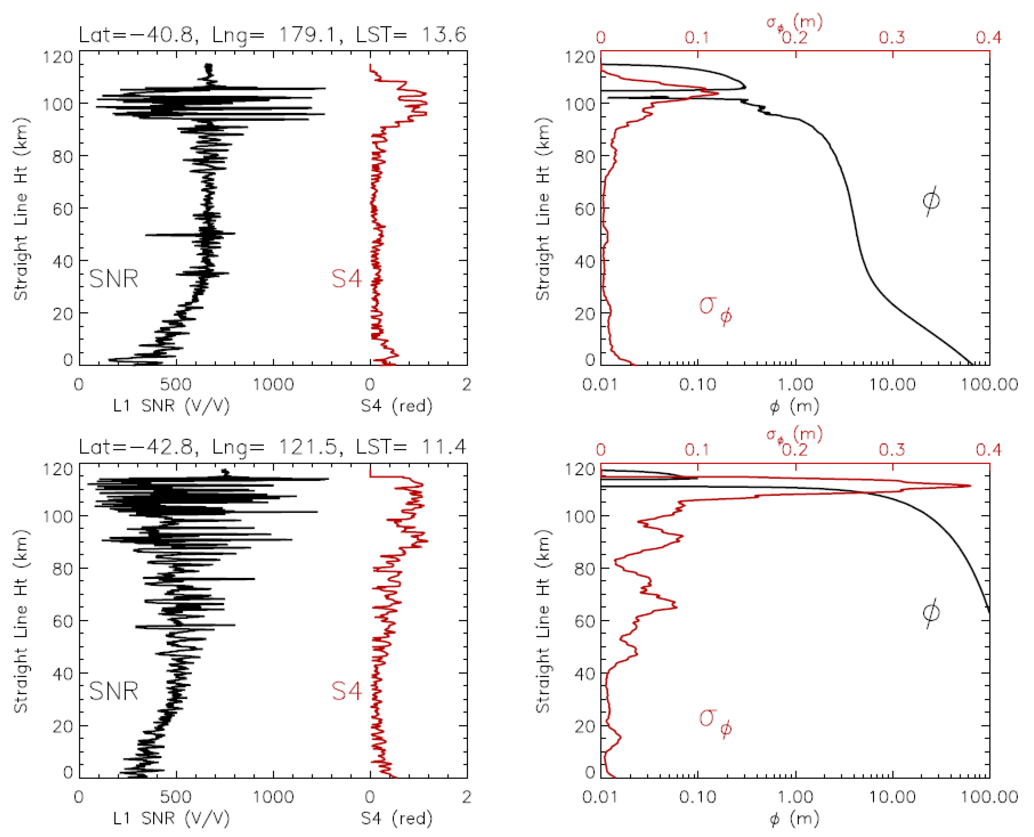
Sporadic-E (E${}_s$) produces strong scintillations in the amplitude and phase of GNSS-RO signals, but the amplitudes of S${}_4$ and ${\sigma }_{\varphi }$ are not necessarily proportional to each other. While an early study [17] compared the SNR and phase perturbations (${\varphi }^{\prime }$), here, we focus on the relationship between S${}_4$ and ${\sigma }_{\varphi }$ exclusively for GNSS-RO L${}_1$ measurements. Figure 1 shows two cases where S${}_4$ appears to be capped at 1.5, while ${\sigma }_{\varphi }$ can reach up to ∼0.4 m.

The first case (top panel in Figure 1) was a typical and popular E${}_s$ event where the S${}_4$ and ${\sigma }_{\varphi }$ oscillations were confined mostly to altitudes of 80–110 km. This narrow height distribution suggests that the E${}_s$ layers were generally thin and horizontally stratified. The RO limb sounding was particularly sensitive to these thin layers, causing strong scintillations when the RO tangent heights were parallel to the layers. However, the scintillation amplitude was significantly reduced at heights lower than the E${}_s$ layer when RO passed through the layers at a slanted angle. A detailed discussion of the geometric smearing effect on the E${}_s$ amplitude by RO can be found in [17].

The second case in Figure 1, although not occurring very frequently, was also an E${}_s$ phenomenon. This event had an extended impact on the scintillation measurements below a ∼115 km tangent height where an E${}_s$ occurred. The extended E${}_s$ can happen when its horizontal extent is large (i.e., 1000 km or greater) and associated with spatial variations of many different scales [17]. Strong gravity waves coupled with planetary wave activities, which can create embedded structures in the E${}_s$ layer, are capable of producing this type of scintillation. Observational evidence (e.g., [29]) and a model illustration [3] all supported such extended impacts from E${}_s$. Alternatively, the extended scintillation could be due to equatorial F-region irregularities, which are known to produce the C-type scintillation [30] displayed here.

2.2. Joint S${}_4$-${\sigma }_{\varphi }$ Histograms

To analyze the GNSS-RO scintillation statistics associated with E${}_s$, we focused on the mid-latitude measurements (−45° latitude) over a month-long period during the local summer (January 2008) at an E-region altitude of 100 km. These parameters were selected to maximize the likelihood of sporadic-E causing scintillation, which is known to occur mostly in the mid-latitudes during the local summer [15,17,18,19] at altitudes near 100 km [20]. While other ionospheric irregularities such as EPBs and polar cap electron density gradients are also known to cause significant satellite-based GNSS scintillation [6], our focus on mid-latitude measurements reduced the likelihood of these other ionospheric irregularities contributing to the observed scintillation (see [3] for more details). However, it did not completely remove the influence of equatorial and polar F-region irregularities. Furthermore, it is known that these ionospheric irregularities have a strong dependence on the local time and other geomagnetic and wind conditions [31,32,33,34,35], but here, we included all measurements taken during the month of interest to increase the total number of data points. By analyzing the scintillation at a single altitude instead of locating the maximum S${}_4$ or ${\sigma }_{\varphi }$ for each occultation, we sampled various regions of the diffraction patterns produced by the E${}_s$ layers with various altitudes centered around 100 km. This sampling was exactly what we attempted to simulate for comparison.

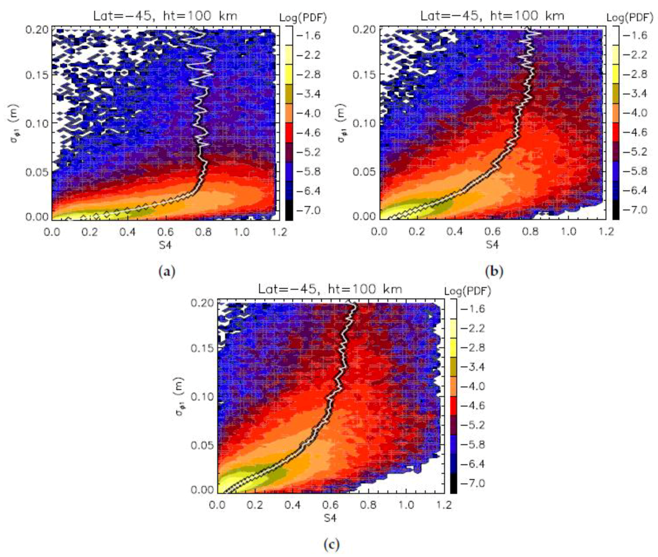
The S${}_4$ saturation from E${}_s$ was further quantified with a joint two-dimensional (2D) S${}_4$-${\sigma }_{\varphi }$ histogram, which clearly showed limited growth by S${}_4$ at large ${\sigma }_{\varphi }$ values. As shown in Figure 2a, where N${}_{cut}$ = 51 was used to extract only thin E${}_s$ layers, the S${}_4$ saturation started to occur at ${\sigma }_{\varphi }\sim 0.03$ m. Although most of the S${}_4$ and ${\sigma }_{\varphi }$ measurements were linearly correlated at small ${\sigma }_{\varphi }$ values, a significant fraction of E${}_s$ had a very large ${\sigma }_{\varphi }$ value that was not linearly proportional to S${}_4$. The S${}_4$ values seemed to have a mean of 0.8 as ${\sigma }_{\varphi }$ increased.

At the larger truncations (i.e., N${}_{cut}$ = 121 and 201), where scintillations from thicker E${}_s$ layers were included, the S${}_4$ saturation was still evident, but it had a gradual transition from unsaturated to saturated. In these cases, the S${}_4$ values tended to approach the same mean at 0.8, and the statistics showed very few samples with S${}_4>1$, especially for N${}_{cut}$ = 201. The reduction in S${}_4$ for the larger windows was caused by the narrow E${}_s$ vertical thicknesses relative to the window lengths, which reduced the S${}_4$ values when scintillation did not occur over the entire window length. For ${\sigma }_{\varphi }$, we saw an increase with increasing window lengths, which was due to larger-scale phase perturbations that were not captured using thin windows. More details on the phase and amplitude perturbations will be provided in Section 3.1. From this, there are benefits to using three different truncation windows for analyzing various intensity and phase perturbations.

3. Gaussian Lens Simulations

To model the scintillation observed in the RO data (Figure 2), the E${}_s$ characteristics from previous studies were randomly sampled with the assumption that the layer acted as a perturbing Gaussian lens. An analytic solution for the electric field pattern following a Gaussian lens follows

$$E\left(X,Z\right)=\sum _{p=0}^{\infty }{\displaystyle \frac{{\left(i{\varphi }_0\right)}^p}{p!}}{\left(1+2ipZ\right)}^{-1/2}exp\left(-{\displaystyle \frac{p{X}^2}{1+2ipZ}}\right),$$

(3)

where E is the complex electric field, $i=\sqrt{-1}$, $X=x/r_0$ is the dimensionless transverse coordinate, and $Z=z/k{r}_0^2$ is the dimensionless coordinate in the propagation direction [36]. Here, $r_0$ is the $1/e$ thickness for the lens and $k=2\pi /\lambda$ is the wavenumber. The Gaussian lens in the transverse plane follows

$$\varphi \left(X\right)={\varphi }_0{e}^{-X^2},$$

(4)

where $\varphi$ is the phase contribution from the lens and ${\varphi }_0$ is the peak lens strength [36]. For our simulations, we used an upper limit of $p=100$ to calculate the complex electric field at a distance of $z=3000$ km after the lens, which is characteristic of RO geometry and the distance traveled to the LEO satellite after reaching the tangent point. A transverse resolution of $\Delta x=4{\lambda }_{L_1}$ was used for the simulations, where ${\lambda }_{L_1}$ was the L${}_1$ wavelength.

While the assumption of a Gaussian lens profile for a sporadic-E layer is certainly an oversimplification, it provides a method to quickly simulate a variety of E${}_s$ lengths, thicknesses, and strengths to analyze the general trends. The complex, turbulent structures observed by incoherent scatter radars [37,38] will provide additional variability and will be explored in Section 4.

The sporadic-E parameters were derived from previous studies for the length, thickness, tilt, and intensity. The length follows a lognormal distribution with a mode of 170 km and $\sigma =0.7$ [39]. We also reduced the lengths by 65%, following the geometry argument in [27] for randomly slicing through sporadic-E layers with horizontal lengths of ∼10 times the horizontal thickness.

The vertical thicknesses follow a lognormal distribution with a mode of 1.5 km and $\sigma =0.4$ [20]. This vertical thickness corresponds to the thickness where the signal intensity reaches 95% of the background intensity within the typical u-shape profile observed for E${}_s$. As observed in Figure 3 and Figure 4, the Gaussian lens is generally thinner than the u-shaped intensity dip, especially for the moderate and stronger lenses. This increase in thickness for the intensity profiles is caused by the negative lens, which diverges the signal away from the lens at large distances. While the relationship between the 95% intensity definition of thickness from [20] and the Gaussian lens thickness defined for simulations is rather complex and requires more research to fully understand, here, we define the vertical thickness as the altitude range between the points where the phase reaches 20% of the lens peak. This 20% value was selected instead of the full width at 1/e to reduce the lens thicknesses and match the observed S${}_4$-${\sigma }_{\varphi }$ trends in Figure 2. Additional research is required to properly map the thicknesses derived in [20] to Gaussian lens thicknesses for simulation or observation. However, this simple mapping provides a starting point for simulation of GNSS-RO statistical observations.

Sporadic-E intensities in the form of foEs were taken from [22], assuming a Gaussian profile with a mean of ∼3 MHz and a standard deviation of ∼1 MHz (estimated from Figures 8 and 9 in [22]). The background E-layer density should be taken into account to properly capture the lens strength magnitudes through conversion of the foEs to an fo$\mu$Es, as outlined in [40], where fo$\mu$Es refers to the metal plasma critical frequency of the E${}_s$ layer. However, we did not explicitly convert the foEs to an fo$\mu$Es here, as we found that the foEs intensity distribution from [22] provided a decent match to the observed S${}_4$-${\sigma }_{\varphi }$ scintillation trends. Furthermore, as fo$\mu$Es calculations require knowledge of the local E-layer densities at the time and location of measurement, it is difficult to calculate an fo$\mu$Es distribution directly from an foEs distribution without additional information. We hope that the statistical approach outlined here helps provide insight into fo$\mu$Es distributions by providing a method for adjusting the distribution to improve agreement between simulations and observations.

The E${}_s$ parameters were converted to effective Gaussian lenses using

$$\begin{array}{cc}\hfill n_p& =\sqrt{1-{\left({\displaystyle \frac{foEs}{f_{L1}}}\right)}^2},\hfill \end{array}$$

(5)

$$\begin{array}{cc}\hfill {\varphi }_0& =\left(n_p-1\right)lk,\hfill \end{array}$$

(6)

where $n_p$ is the index of refraction at the center of the E${}_s$ layer, l is the horizontal length of the layer, $f_{L1}$ is the GPS L${}_1$ frequency of 1575.42 MHz, and k is the L${}_1$ wavenumber. With $n_p<1$, ${\varphi }_0<0$, which creates a negative lens. Here, we ignored the background ionosphere to simplify the simulations, and the E${}_s$ tilts were not included to focus on the moderate-to-strong scintillation trends. As shown in [20], layer tilts significantly reduced the amplitude scintillation at the LEO measurement plane, which introduced additional data points near the origin of our S${}_4$-${\sigma }_{\varphi }$ histograms. As these points did not significantly contribute to the moderate-to-strong scintillation trends observed in Figure 2, they were ignored for this analysis.

3.1. Simulation Examples

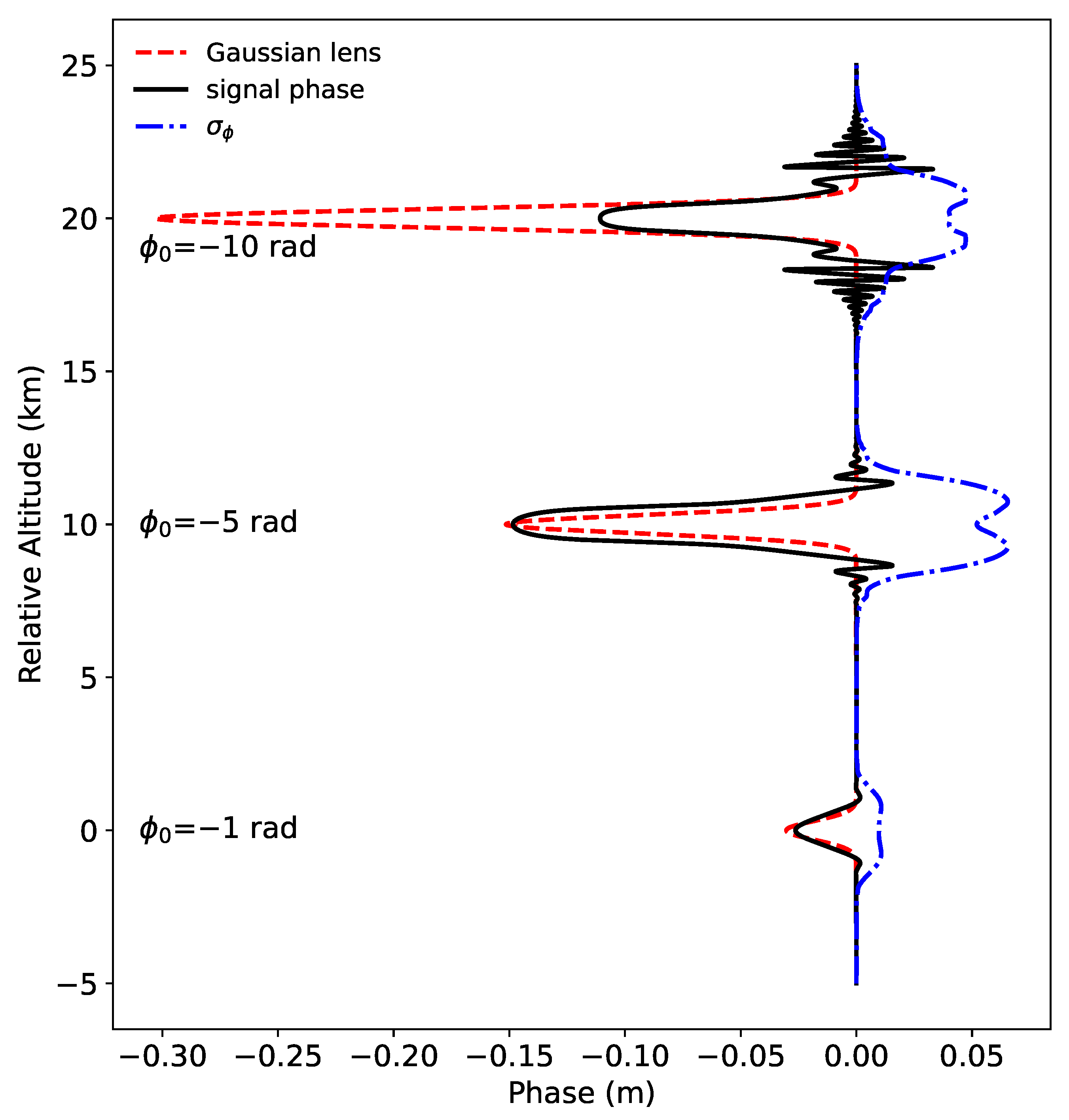
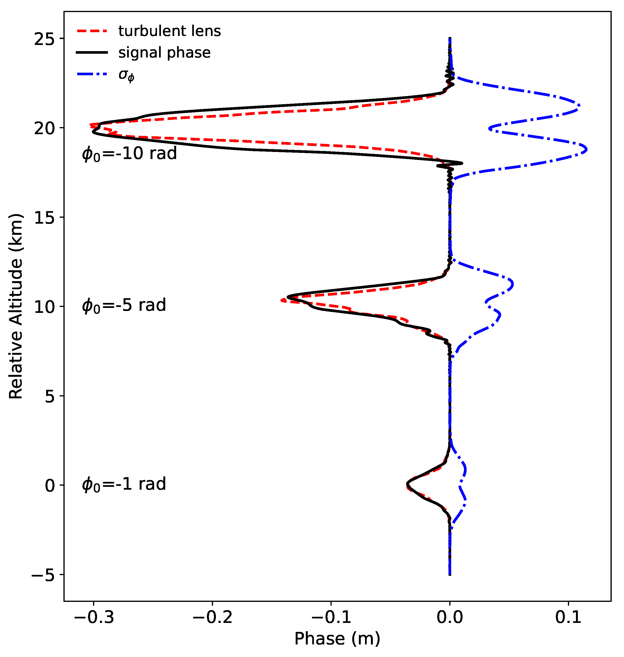
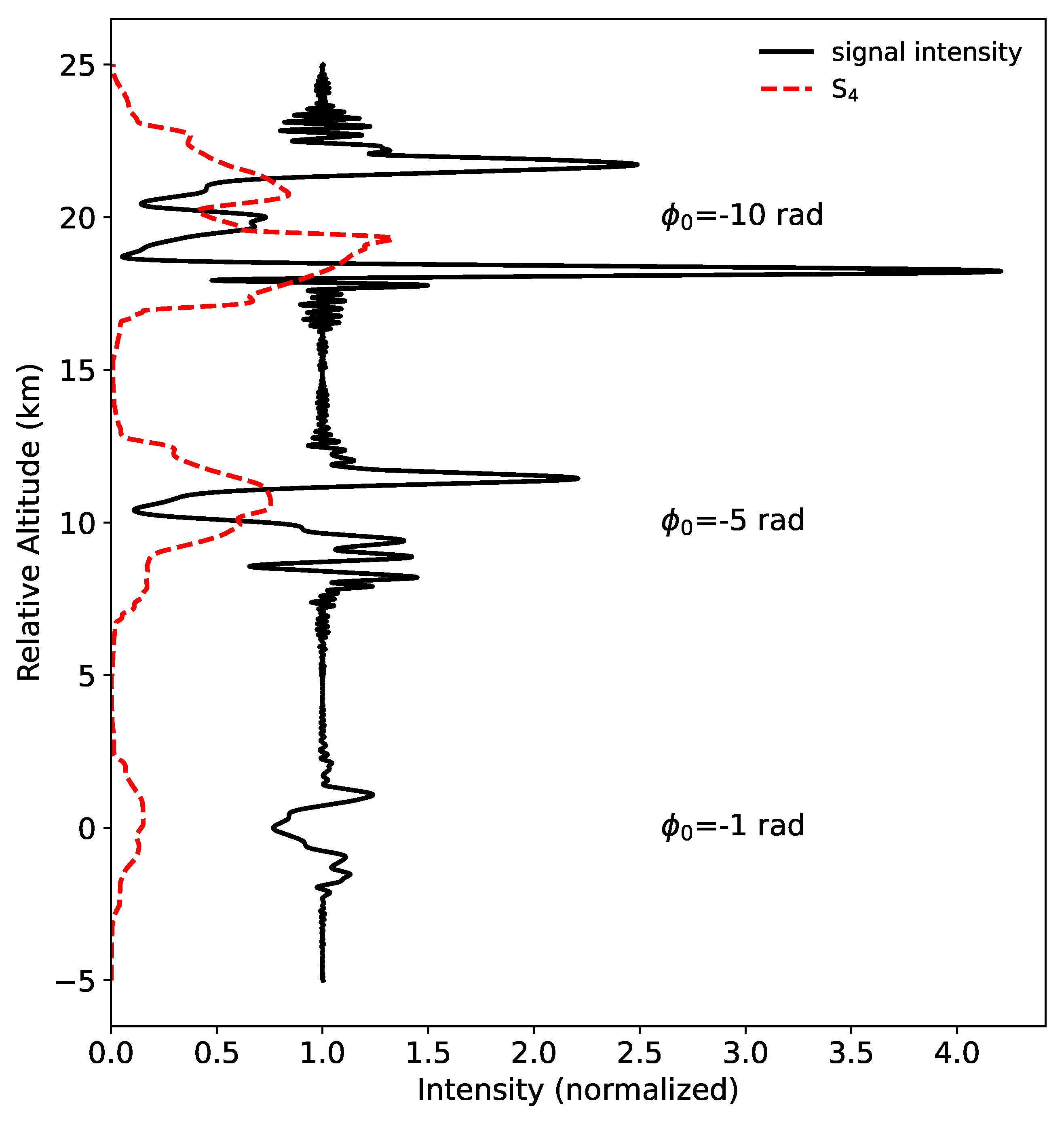
Examples of the Gaussian lens simulations are displayed in Figure 3 and Figure 4 for the phase and intensity of the GPS L${}_1$ signal, respectively, as measured at the LEO measurement plane after propagating through a sporadic-E layer with a vertical thickness of 1.5 km. Three varying lens strengths are displayed to show the different scintillation responses, using a 2.2 km window (N${}_{cut}$ = 51) to calculate S${}_4$ and ${\sigma }_{\varphi }$. The lens strengths were −1 rad (−3 cm), −5 rad (−15 cm), and −10 rad (−30 cm), showing weak, moderate, and strong lensing, respectively. For perspective, the −5 rad lens strength may correspond to an E${}_s$ layer with a 3.4 MHz foEs and a length of 65 km. As observed in Figure 3, the measured signal phase closely tracked the Gaussian lens for the weak and moderate lenses, but significant phase scintillation reduced the measured phase for the strong lens. Interestingly, while the scintillation on the edges of the lens was most severe for the strong lens, the largest ${\sigma }_{\varphi }$ was observed for the moderate lens scenario with a peak of ∼6 cm. This counter-intuitive result was due to the large phase gradient from the lens that was mostly captured by the moderate lens, but it was less severe for the strong lens because of the phase scintillation observed at the edges, which reduced the peak phase measured in the lens. These results indicate that thin, strong lenses can produce relatively low peak ${\sigma }_{\varphi }$ values, but the phase scintillation at the edges of the lenses will be enhanced.

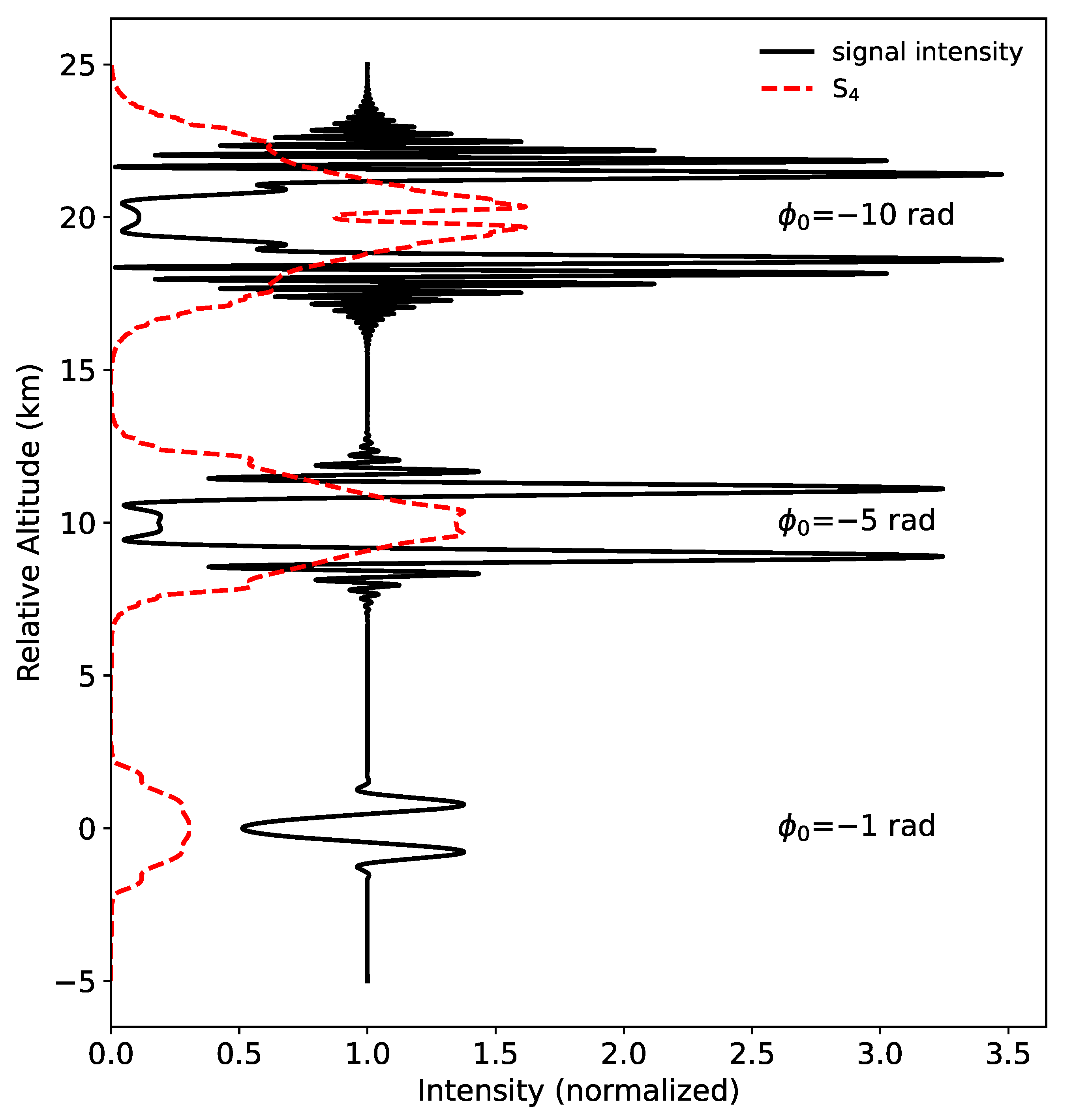
The signal intensities at the LEO measurement plane for the same lenses are displayed in Figure 4. Here, the characteristic U-shaped profile described in [20] is present for the moderate and strong lenses, where the low intensity region at the bottom of the U shape was caused by the negative lensing effect of the E${}_s$ layers. Additionally, the ringing around the u-shape fade is due to diffraction [20]. However, the weak lens did not produce a strong diffraction pattern, and only the beginning of a U-shaped pattern was present. S${}_4$ showed elevated peaks of 1.3 for the moderate lens and 1.5 for the strong lens, with a relatively low peak of approximately 0.3 for the weak lens. In the center of the moderate and strong profiles, the S${}_4$ magnitude was elevated by the decreased intensity mean at the center of the U-shaped profile. For the S${}_4$ techniques calculated using a longer running average of the background intensity, such as those provided by the COSMIC Data Analysis and Archive Center (CDAAC) [28], the S${}_4$ calculated over one-second intervals (50 points for 50 Hz data) would be nearly equal to the standard deviation of the normalized intensity.

Following the results from [27], the peak S${}_4$ plateaued for the moderate-to-strong lenses, and the roughly linear peak S${}_4$ relationship with the lens strength was mostly observed for the weak-to-moderate lenses. Additionally, the vertical lens thickness played a large role in the phase and amplitude scintillation, with thinner lenses generally causing more scintillation in both phase and amplitude. However, as discussed previously, ${\sigma }_{\varphi }$ also depends on the large phase perturbation induced directly by the E${}_s$ layer and not strictly the scintillation from diffraction. These examples help to interpret the statistical results outlined below.

3.2. Simulated Statistics

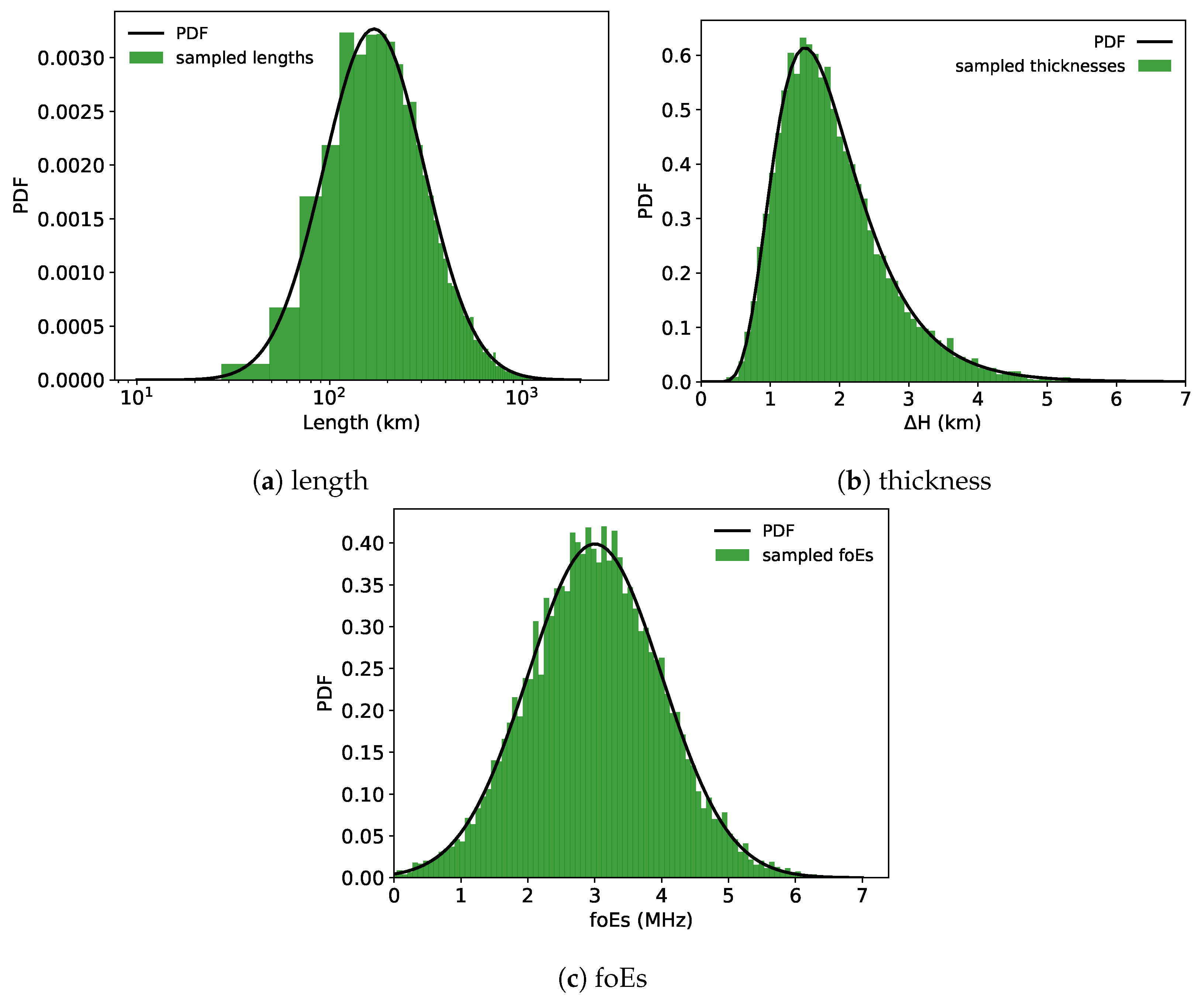
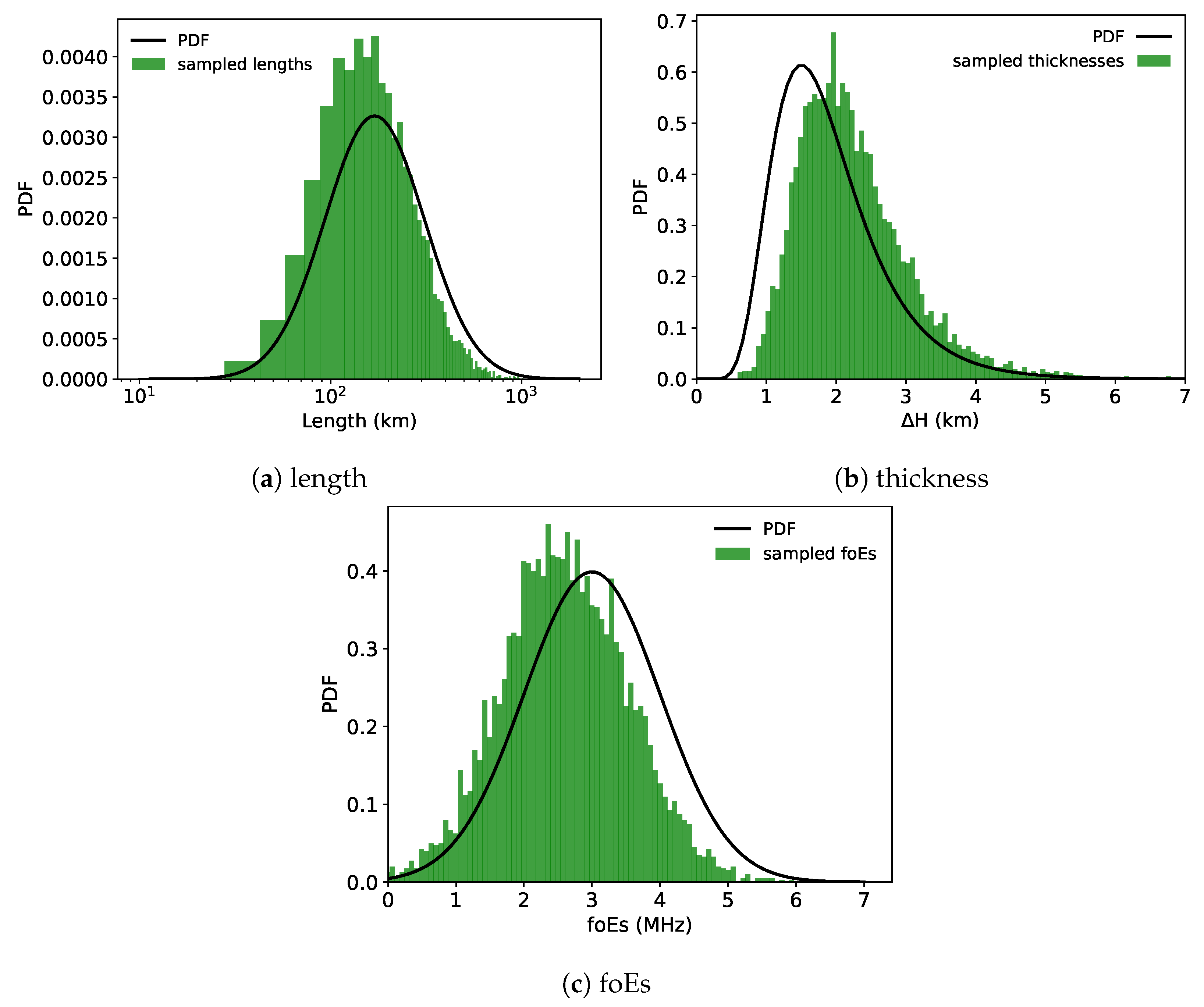
In an attempt to reproduce the observations displayed in Figure 2, the E${}_s$ length, vertical thickness, and foEs distributions were randomly sampled 10,000 times, and the resulting electric field profiles in the LEO measurement plane ($z=3000$ km) were stored for each of the 10,000 simulations. Histograms of the sampling along with the distributions are displayed in Figure 5a for the length, Figure 5b for the vertical thickness, and Figure 5c for the foEs.

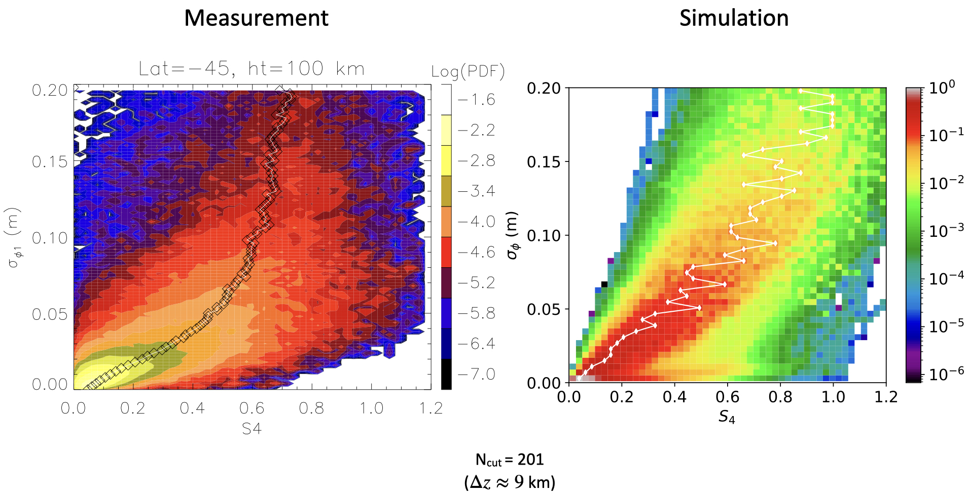
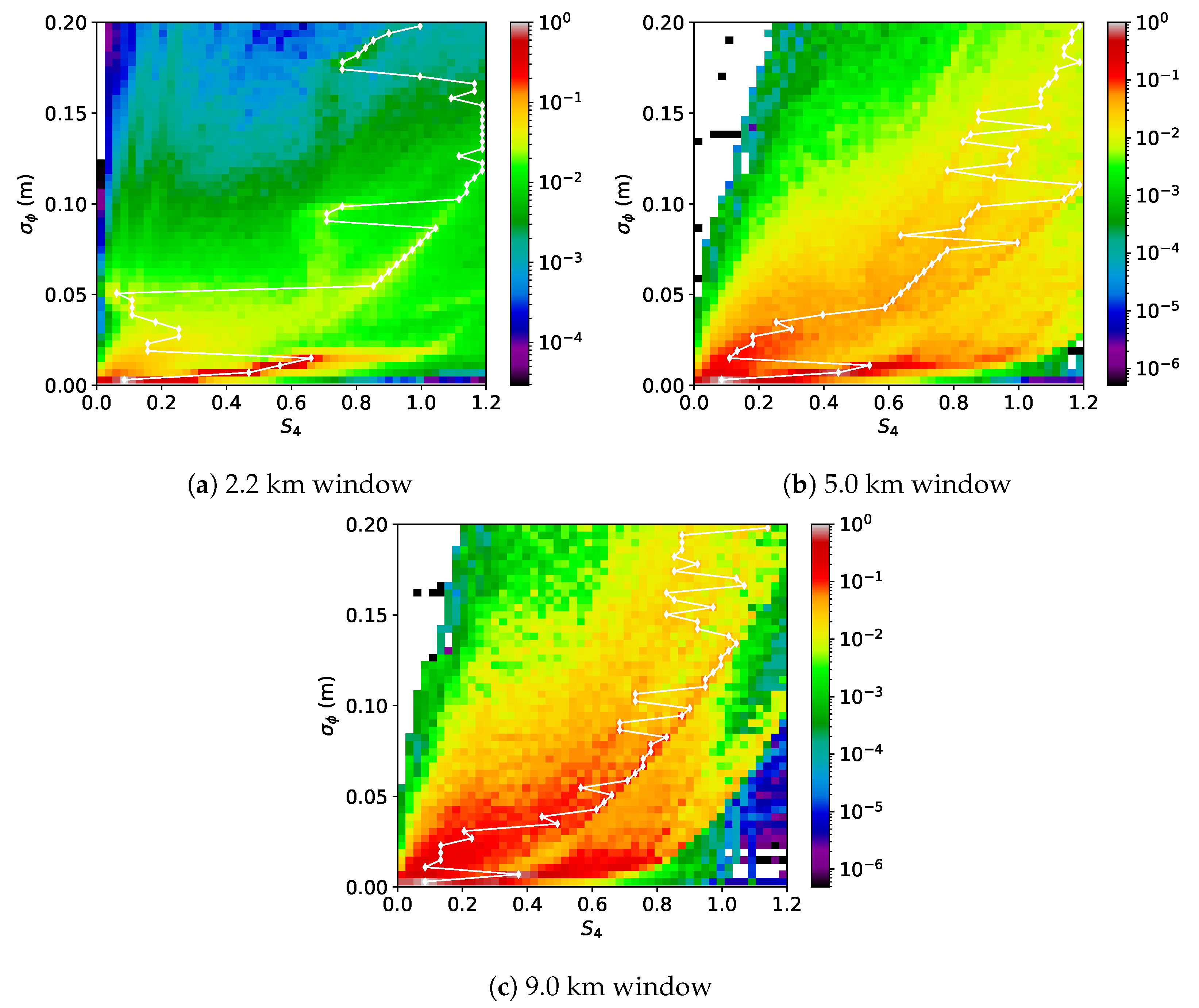
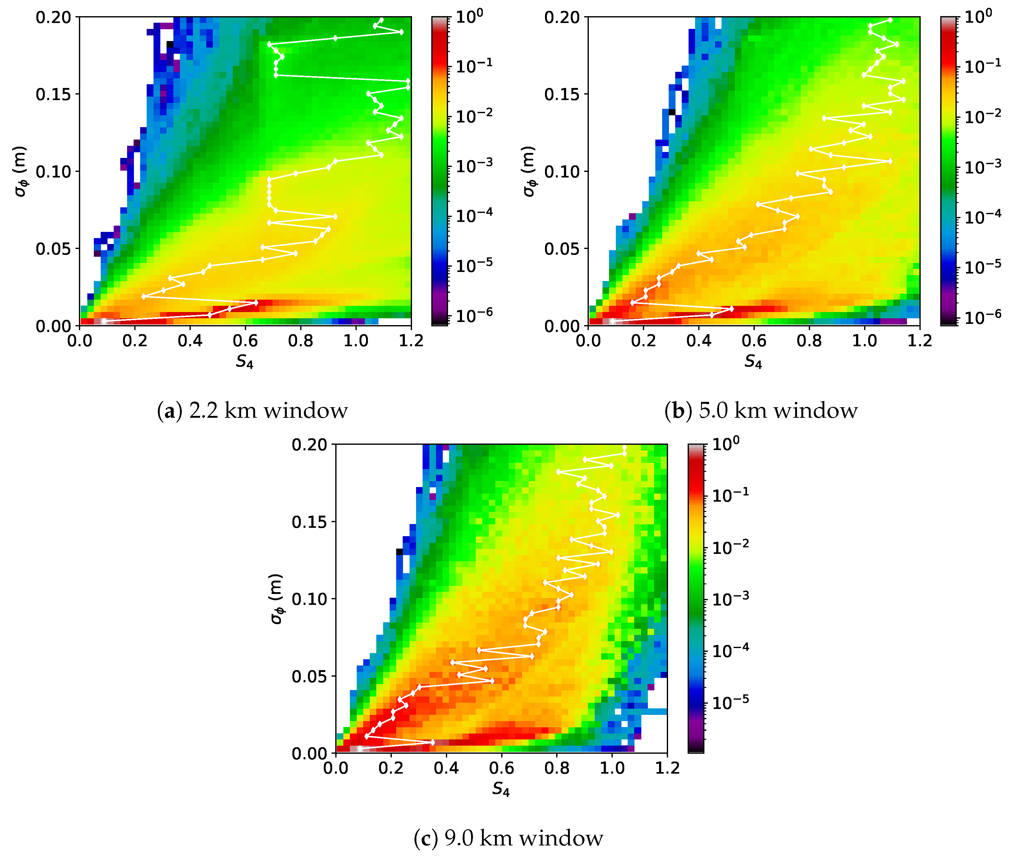
Joint S${}_4$-${\sigma }_{\varphi }$ histograms of the simulated S${}_4$ and ${\sigma }_{\varphi }$ at the LEO measurement plane are displayed in Figure 6. Each grid point in the measurement plane was used as a single data point to create the histogram. Extremely low values (below 0.001) were removed for both S${}_4$ and ${\sigma }_{\varphi }$ to improve readability. The majority of points occurred in the region of S${}_4<0.3$ and ${\sigma }_{\varphi }<0.02$ m, corresponding to weak intensity and phase fluctuations, respectively. This region corresponds to the weak lens simulations in Figure 3 and Figure 4.

Outside of this weak lens region, there were three regions of interest. The first most noticeable region was caused by significant phase scintillation with elevated S${}_4$ and low ${\sigma }_{\varphi }$. When strong phase scintillation occurred, the peak phase perturbation magnitude was reduced, which in turn reduced the ${\sigma }_{\varphi }$ peak, as displayed in Figure 3. In this region, both phase and amplitude scintillation are important, and techniques such as those outlined in [17,19,22] will work well, while techniques relying on phase perturbation alone will struggle with properly characterizing the layer. With the exception of the 2.2 km window, the simulations showed significant counts in this region while the observations (Figure 2) did not. This indicates that the simulations were oversampling the strong-thin regions, and a method to reduce this sampling is presented in Section 5.

The second region of interest was produced by the moderate lenses, resulting in a roughly linear increase in ${\sigma }_{\varphi }$ with respect to S${}_4$. For the 2.2 km window, this moderate lens zone was much weaker than the strong scintillation zone, but the strong scintillation linear trend from the origin to S${}_4\approx 0.7$, ${\sigma }_{\varphi }\approx 0.02$ m roughly matched the observations in Figure 2. The moderate lens region was more obvious for the 5.0 km and 9.0 km windows, with a $\Delta {\sigma }_{\varphi }/\Delta S_4$ slope of 0.05/0.6 m for both windows. These slopes were in line with the observed slopes from the origin to ${\sigma }_{\varphi }\approx 0.05$ m, although the observations showed a slightly elevated slope of 0.05/0.5 m for the 9.0 km window.

However, the simulated moderate lens region extended throughout S${}_4\approx 1.2$, which was not observed in the GNSS-RO measurements. Instead, Figure 2 shows the S${}_4$ plateau between 0.6 and 0.8. This difference was likely due to the assumption of a Gaussian lens for the E${}_s$ layers, which was certainly an oversimplification, as shown by the incoherent scatter radar measurements (e.g., [37,38]). The realistic E${}_s$ layers were patchy and billowy, which was caused by the Kelvin–Helmholtz instability [41], reducing the ideal strong lensing and also introducing additional perturbations and scintillation caused by the billows. The Gaussian lens’s focusing diffraction pattern is capable of producing very large peak intensity scintillation, while the billowy layers from turbulence are not capable of producing the same focusing. This important point will be explored further in Section 4.

Finally, the third zone of interest was characterized by elevated ${\sigma }_{\varphi }$ and low S${}_4$ (Figure 6a) due to thicker layers with relatively weak lens strengths. These thicker, weaker layers caused phase perturbations without causing significant diffraction in the signal intensity. The GPS-RO techniques relying on phase perturbation (e.g., [18,25]) will work well in this region, while the techniques relying on the signal intensity (e.g., [19,22]) will have difficulty characterizing these thicker, weaker layers.

While the simulations reported here were strictly for GNSS-RO geometries, it must be noted that many previous studies have compared and validated RO techniques for monitoring sporadic-E with ground-based ionosondes [19,21,25,26]. The foEs distribution [22] was derived from RO observations with an empirical fit to ionosonde measurements, and the length distribution was taken from a topside sounder (Explorer 20) [39]. There is certainly room for improvement in GNSS-RO techniques for monitoring sporadic-E, but the general agreement with ground-based sensors provides confidence in the results obtained only from GNSS-RO observations.

4. Simulations Including Turbulence

Following [42], the spectral density function ${\mathrm{\Phi }}_{\delta n}\left(k\right)$ for random variations in the index of refraction $\delta n\left(\overrightarrow{r}\right)$ can be described by

$${\mathrm{\Phi }}_{\delta n}\left(k\right)=\langle \delta n^2\rangle Q\left(k\right)$$

(7)

where $\langle \delta n^2\rangle$ is the refractive index variance and $Q\left(k\right)$ is the Shkarofsky [43] spectral density function:

$$Q\left(k\right)={\left({\displaystyle \frac{4\pi }{k_s{k}_L}}\right)}^{3/2}{\displaystyle \frac{{\left(\sqrt{1+{(k/k_L)}^2}\right)}^{-(\nu +1/2)}{K}_{\nu +1/2}\left(2{\displaystyle \frac{k_L}{k_s}}\sqrt{1+{(k/k_L)}^2}\right)}{K_{\nu -1}\left(2{\displaystyle \frac{k_L}{k_S}}\right)}}.$$

(8)

Here, $k_S$ corresponds to the inner scale (smallest structure), $k_L$ corresponds to the outer scale (largest structure), $K_{\nu }$ is the modified Bessel function, and $\nu$ is the power law index parameter. Additionally, we have

$$\langle \delta n^2\rangle ={\displaystyle \frac{\mathrm{\Gamma }\left(\nu -1\right)C_s}{{\left(4\pi \right)}^{3/2}\mathrm{\Gamma }(\nu +1/2)k_L^{2\nu -2}}},$$

(9)

where $C_s$ is the turbulent strength parameter.

To include a turbulence spectrum into our simulations, we used the following conditions: $k_S=2\pi /100$ rad/m, $k_L=2\pi /\Delta x$ rad/m where $\Delta x$ is the vertical thickness of the layer, $\nu =4/3$ for the Kolmogorov turbulence, and $C_s={10}^{-8}$. A Kolmogorov power law was selected based on the results in [44], and the value of $C_s$ was adjusted to improve the simulations agreement with the observations displayed in Figure 2 while also producing vertical refractivity profiles with variations similar to those observed for the horizontally integrated E${}_s$ profiles from the ISR measurements as displayed in [37]. This turbulence was added to the initial Gaussian lens by generating complex frequency samples of the Shkarofsky spectrum using a normal distribution with a standard deviation of one and a mean of zero for both the real and imaginary components. The Fourier transform of these spectral random realizations provided random fluctuations in space that were added to the original Gaussian lens to provide a turbulent sporadic-E layer:

$$n_{turb}(x,z)=n_0(x,z)\left[1+\delta n\left(x\right)\right],$$

(10)

where $n_{turb}(x,z)$ is the two-dimensional index of refraction with the inclusion of turbulence, $n_0(x,z)$ is the original refractive index profile, and $\delta n\left(x\right)$ is the random index of refraction variation in the vertical (transverse) direction. Here, we used the same vertical $\delta n\left(x\right)$ for all z in the horizontal (propagation) direction to focus on vertical lens irregularities.

Example phase and amplitude profiles for turbulent lenses are displayed in Figure 7 and Figure 8. The same lens strengths of −1, −5, and −10 radians used for the Gaussian lenses in Figure 3 and Figure 4 are analyzed here. However, the vertical thickness was increased to 2.5 km to clearly see the turbulence. The phase profiles showed similar behavior to the Gaussian lenses, with the exception of reduced phase scintillation for the −10 radian lens due to the thicker vertical thickness that reduced the overall vertical gradient in the index of refraction. A slight asymmetry was observed for the −10 radian lens, with a stronger asymmetry observed for the −5 rad lens. While the phase profiles were similar to the Gaussian lenses, the amplitude profiles were significantly perturbed (Figure 8). This was most obvious for the −5 and −10 radian lenses, which showed large asymmetries in the idealized U-shaped profiles. This asymmetry was a result of the asymmetric lens caused by the inclusion of turbulence. The asymmetric U-shaped profile presented here is commonly measured in GNSS-RO observations (e.g., Figure 1), resulting from the small scale structures observed in E${}_s$ layers. Additionally, the strong S${}_4$ caused by lens focusing was reduced in the turbulent lenses because of the lens imperfections. This reduced focusing ultimately resulted in the S${}_4$ plateau observed in Figure 1.

It must be noted here that many GNSS-RO observations of sporadic-E show multiple layers [45]. These multi-layered structures result in either multiple U shapes or a blend caused by the interference of the two diffraction patterns. Examples of these multi-layered profiles can be found in previous studies (e.g., Figure 3 of [20]) and throughout the CDAAC catalog (e.g., atmPhs_C001.2010.029.01.35.G14_2010.2640_nc and atmPhs_C002.2008.001.00. 28.G04_2013.3520_nc). The simplified modeling approach taken here did not account for these multi-layered structures, as we were focused on the scintillation produced by single layers. While the multi-layered events with sufficient altitude spread would not change the scintillation statistics of the individual layers, the interfering diffraction patterns were not accounted for in this study.

After the turbulence was added to the Gaussian lens, an analytic solution to the electric field (i.e., Equation (3) for the Gaussian lens) no longer existed, and the electric field at the GNSS-RO measurement plane had to be calculated using a numerical technique. Here, we used the multiple-phase screen approach due to the long propagation distance of 3000 km after the perturbing layer. This multiple-phase screen approach is commonly used for RO propagation through sporadic-E layers [17,20,27], and more information on the technique can be found in [42,46]. Specifically, we used a transverse (vertical) grid spacing of 76 cm (four L${}_1$ wavelengths) for a total transverse length of 50 km. In the propagation (horizontal) direction, we took 1000 equal steps through the E${}_s$ layer followed by ∼20 km steps after the layer for a total propagation distance of 3000 km.

Using the same distributions implemented for Figure 6 with the addition of turbulence provided the results displayed in Figure 9. The linear slopes were similar to the slopes observed for the Gaussian lens, but plateauing of S${}_4\approx 1.0$ better matched the observations (Figure 2). This was due to a reduction in the Gaussian lenses focusing with the lens “imperfections” added by the turbulence. Additionally, the 9.0 km window $\Delta {\sigma }_{\varphi }/\Delta S_4$ slope from the origin was increased to 0.05/0.5 m, which matched the observed slope better than the Gaussian lens simulations. The similarity of these simulations to the observations supports previous sporadic-E measurements that showed the turbulent nature of these layers [37,38]. Including a relatively small degree of turbulence in our simulations provided more realistic sporadic-E layers and improved our agreement with the GNSS-RO observations.

While the inclusion of turbulence helped to reduce the high ${\sigma }_{\varphi }$ and S${}_4$ region caused by focusing, the strong phase scintillation region with strong S${}_4$ and low ${\sigma }_{\varphi }$ remained more enhanced than the observations suggest. Similar to the Gaussian lens results, the 2.2 km window showed reasonable agreement with the observed $\Delta {\sigma }_{\varphi }/\Delta S_4$ slopes from the origin, but the 5.0 and 9.0 windows did not show this enhancement. This implies that we were oversampling the strong, thin layers with large vertical gradients in the index of refraction, and some physical limitation on the coupled E${}_s$ characteristics may have existed that was unaccounted for in our uncoupled random sampling.

5. Diffusion-Limited

The region of elevated S${}_4$ and low ${\sigma }_{\varphi }$ observed in our simulations (Figure 6 and Figure 9) was not present in the observations displayed in Figure 2, indicating that the strong, thin layers were oversampled from the length, strength, and vertical distributions. To limit the number of strong, thin lenses in an attempt to improve agreement with the observations, we removed the randomly sampled layers with ${\varphi }_0/r_0^2>13.5$ rad/km${}^2$. This threshold value was obtained by averaging the ratios obtained for the ${\varphi }_0$ values, where various vertical thicknesses in the range of $0.5\le r_0\le 1.5$ km began to show significant phase scintillation. Here, we define significant phase scintillation as a peak measured phase difference of greater than 30% from the applied phase, illustrated by the black and red lines in Figure 3. Physically, this limit on ${\varphi }_0/r_0^2$ may be related to a diffusion limited layer as $D_i{d}^2{n}_i/d{x}^2\propto {\varphi }_0/r_0^2$ at the center of the layer, where $D_i$ is the diffusion coefficient for metal ions, $n_i$ is the metal ion density, and x is in the vertical direction. Ion convergence caused by wind shears is counteracted by this vertical diffusion such that the final layer characteristics will be dependent on both processes [8]. Layers that become too strong and thin will experience elevated diffusion that will ultimately place a limit on the allowed ${\varphi }_0/r_0^2$ ratio.

Using this diffusion limit on the randomly sampled distributions resulted in the remaining parameters displayed in Figure 10. Out of the 10,000 initial samples, 4383 layers with ${\varphi }_0/r_0^2>13.5$ rad/km${}^2$ were removed. Compared with Figure 5, the layers with elevated values for length or foEs (${\varphi }_0$ is proportional to the length-foEs${}^2$ product) and low $r_0$ were removed from the distributions.

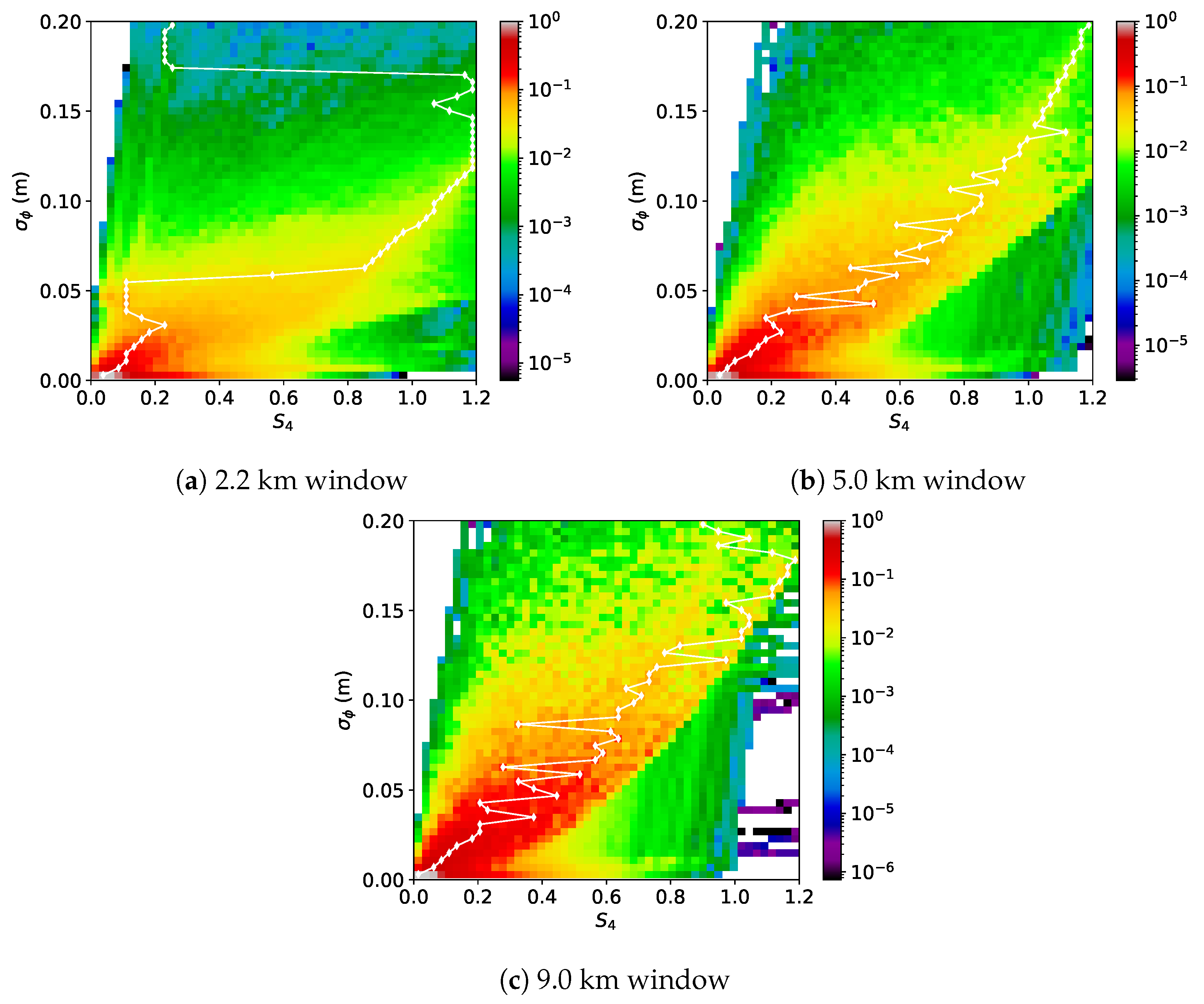
The simulated S${}_4$-${\sigma }_{\varphi }$ histograms for these diffusion-limited layers are displayed in Figure 11. Compared with the original distributions used to create Figure 6, the strong phase scintillation region with elevated S${}_4$ and low ${\sigma }_{\varphi }$ was greatly reduced. Similarly, the S${}_4$-${\sigma }_{\varphi }$ histograms for the turbulent lenses were also improved by the removal of layers with ${\varphi }_0/r_0^2>13.5$ rad/km${}^2$ (Figure 12). While the strong phase scintillation region was not completely removed in the simulations, inclusion of the diffusion-limited threshold on the ${\varphi }_0/r_0^2$ ratio significantly improved agreement with the observations.

The threshold enforced here was selected to show a proof of concept, but placing physical thresholds on the randomly sampled distributions should be enforced to ensure that unrealistic sporadic-E layers are not produced. Determination of these thresholds requires insight into the coupling between each of the parameters, which we treated as independent up to this point. Alternatively, the reduction of longer, thinner, and stronger layers may indicate that the E${}_s$ distributions used here require adjustment to match the observations. For the length distribution, the authors of [23] found that strong layers have a median length of 100 km, which is a reduction from the 170 km mode used here from [39]. Additionally, taking the background E-layer into account through a conversion of foEs to fo$\mu$Es as outlined in [40] would help to reduce the effective lens strengths, since ${\varphi }_0\propto$ length-foEs${}^2$. Certainly, additional research is warranted to help improve the E${}_s$ distributions and to determine the coupling characteristics.

6. Conclusions

A statistical view of GNSS-RO phase and amplitude scintillation at an E-region altitude in the mid-latitudes during the local summer indicates that sporadic-E is likely the primary cause of the unique S${}_4$-${\sigma }_{\varphi }$ trends. The GNSS-RO observations showed a nearly linear trend in joint two-dimensional S${}_4$-${\sigma }_{\varphi }$ histograms until the S${}_4$ saturated near 0.8. To understand the trends, 10,000 RO simulations through sporadic-E layers were performed using length, intensity, and vertical thickness distributions from previous research with the assumption that the E${}_s$ layer acted as a Gaussian lens. This simplified view of the layers provides insight into different scintillation statistics for weak, moderate, and strong lenses.

Using the Gaussian lens assumption, a roughly linear $\Delta {\sigma }_{\varphi }/\Delta {\mathrm{S}}_4$ slope from the origin to ${\sigma }_{\varphi }\approx 0.05$ m was observed in both the observations and simulations. In the simulations, this trend was produced strictly by E${}_s$ layers, which implies that the observed GNSS-RO scintillation was also likely caused by E${}_s$. While the Gaussian layer simulations showed agreement with the primary trends, a region of elevated ${\sigma }_{\varphi }$ and S${}_4$ was present in the simulations but not the observations. This elevated S${}_4$-${\sigma }_{\varphi }$ was caused by focusing from these idealized lenses. In reality, the E${}_s$ layers were turbulent and billowy. Therefore, we included Kolmogorov turbulence by adding random realizations of a Shkarofsky spectral density function to perturb the idealized Gaussian lenses. The addition of these random turbulence fluctuations made the E${}_s$ layers more physically realistic, which in turn improved agreement with the observations by removing the large number of points in the elevated ${\sigma }_{\varphi }$ and S${}_4$ region. Additionally, a plateau of S${}_4\approx 1.0$ was produced by these turbulent layers, which better matched the observed trends.

Simulations using the original distributions without constraints on the coupled layer parameters showed large counts with significant phase scintillation (elevated S${}_4$ and low ${\sigma }_{\varphi }$) produced by strong, thin lenses. This strong phase scintillation region was not present in the observations, which indicated an oversampling of these strong, thin layers. To reduce this oversampling, a threshold was placed on the ${\varphi }_0/r_0^2$ ratio which was proportional to the ion diffusion rates. After placing a limit on this ratio, counts in the elevated S${}_4$ and low ${\sigma }_{\varphi }$ region were significantly reduced, resulting in better agreement with the observations and implying that there may be a diffusion limit on E${}_s$ layers. The improvement was best illustrated by the 2.2 km window simulations, likely due to the narrow window being more sensitive to small-scale phase fluctuations.

This research provides a new method for interpreting GNSS-RO results in bulk through large numbers of simulations guided by predefined probability distribution functions. For future work, the distributions can be adjusted to find the best fits to the statistical observations and improve our understanding of the sporadic-E layer characteristics. However, it must be noted that certain ambiguities arise with respect to the length × foEs${}^2$ product contributing to the strength of the lens, and the diffraction pattern is also highly dependent on the lens thickness, which requires physically realistic bounds and starting points placed on the distributions using previous E${}_s$ measurements. Improving the turbulence estimates and implementation can also help improve agreement and provide insight into the complex layer structure. Finally, it may be possible to apply this approach to equatorial and polar observations to enhance characterization of the ionospheric disturbances in these regions. While the scale sizes, general characteristics, and challenges of equatorial and polar observations are markedly different than those for mid-latitude E${}_s$, a statistical scintillation approach taking advantage of RO geometry provides a complementary dataset to the traditional ground-based GNSS measurements.

References

- Groves, K.; Basu, S.; Quinn, J.; Pedersen, T.; Falinski, K.; Brown, A.; Silva, R.; Ning, P. A comparison of GPS performance in a scintillation environment at Ascension Island. In Proceedings of the 13th International Technical Meeting of the Satellite Division of The Institute of Navigation (ION GPS 2000), Salt Lake City, UT, USA, 19–22 September 2000; pp. 672–679. [Google Scholar]
- Dubey, S.; Wahi, R.; Gwal, A. Ionospheric effects on GPS positioning. Adv. Space Res. 2006, 38, 2478–2484. [Google Scholar] [CrossRef]
- Wu, D.L. Ionospheric S4 scintillations from GNSS radio occultation (RO) at slant path. Remote Sens. 2020, 12, 2373. [Google Scholar] [CrossRef]
- Schrijver, C.J.; Kauristie, K.; Aylward, A.D.; Denardini, C.M.; Gibson, S.E.; Glover, A.; Gopalswamy, N.; Grande, M.; Hapgood, M.; Heynderickx, D.; et al. Understanding space weather to shield society: A global road map for 2015–2025 commissioned by COSPAR and ILWS. Adv. Space Res. 2015, 55, 2745–2807. [Google Scholar] [CrossRef]
- Kintner, P.M.; Ledvina, B.M.; De Paula, E. GPS and ionospheric scintillations. Space Weather 2007, 5. [Google Scholar] [CrossRef]
- Yue, X.; Schreiner, W.S.; Pedatella, N.M.; Kuo, Y.H. Characterizing GPS radio occultation loss of lock due to ionospheric weather. Space Weather 2016, 14, 285–299. [Google Scholar] [CrossRef] [Green Version]
- Whitehead, J. Recent work on mid-latitude and equatorial sporadic-E. J. Atmos. Terr. Phys. 1989, 51, 401–424. [Google Scholar] [CrossRef]
- Haldoupis, C. A tutorial review on sporadic E layers. In Aeronomy of the Earth’s Atmosphere and Ionosphere; Springer Science & Business Media: Berlin/Heidelberg, Germany, 2011; pp. 381–394. [Google Scholar]
- Mathews, J. Sporadic E: Current views and recent progress. J. Atmos. Sol.-Terr. Phys. 1998, 60, 413–435. [Google Scholar] [CrossRef]
- Smith, E.K. Worldwide Occurrence of Sporadic E.; US Department of Commerce, National Bureau of Standards: Washington, DC, USA, 1957; Volume 582.
- Matsushita, S.; Reddy, C. A study of blanketing sporadic E at middle latitudes. J. Geophys. Res. 1967, 72, 2903–2916. [Google Scholar] [CrossRef]
- Whitehead, J. The structure of sporadic E from a radio experiment. Radio Sci. 1972, 7, 355–358. [Google Scholar] [CrossRef]
- Pignalberi, A.; Pezzopane, M.; Zuccheretti, E. A spectral study of the mid-latitude sporadic E layer characteristic oscillations comparable to those of the tidal and the planetary waves. J. Atmos. Sol.-Terr. Phys. 2015, 122, 34–44. [Google Scholar] [CrossRef]
- Yadav, V.; Kakad, B.; Bhattacharyya, A.; Pant, T. Quiet and disturbed time characteristics of blanketing Es (Esb) during solar cycle 23. J. Geophys. Res. Space Phys. 2017, 122, 11–591. [Google Scholar] [CrossRef]
- Merriman, D.; Nava, O.; Dao, E.; Emmons, D. Comparison of seasonal foEs and fbEs occurrence rates derived from global Digisonde measurements. Atmosphere 2021, 12, 1558. [Google Scholar] [CrossRef]
- Hocke, K.; Igarashi, K.; Nakamura, M.; Wilkinson, P.; Wu, J.; Pavelyev, A.; Wickert, J. Global sounding of sporadic E layers by the GPS/MET radio occultation experiment. J. Atmos. Sol.-Terr. Phys. 2001, 63, 1973–1980. [Google Scholar] [CrossRef]
- Wu, D.L.; Ao, C.O.; Hajj, G.A.; de La Torre Juarez, M.; Mannucci, A.J. Sporadic E morphology from GPS-CHAMP radio occultation. J. Geophys. Res. Space Phys. 2005, 110. [Google Scholar] [CrossRef] [Green Version]
- Chu, Y.H.; Wang, C.; Wu, K.; Chen, K.; Tzeng, K.; Su, C.L.; Feng, W.; Plane, J. Morphology of sporadic E layer retrieved from COSMIC GPS radio occultation measurements: Wind shear theory examination. J. Geophys. Res. Space Phys. 2014, 119, 2117–2136. [Google Scholar] [CrossRef]
- Arras, C.; Wickert, J. Estimation of ionospheric sporadic E intensities from GPS radio occultation measurements. J. Atmos. Sol.-Terr. Phys. 2018, 171, 60–63. [Google Scholar] [CrossRef]
- Zeng, Z.; Sokolovskiy, S. Effect of sporadic E clouds on GPS radio occultation signals. Geophys. Res. Lett. 2010, 37. [Google Scholar] [CrossRef]
- Niu, J.; Weng, L.; Meng, X.; Fang, H. Morphology of Ionospheric Sporadic E Layer Intensity Based on COSMIC Occultation Data in the Midlatitude and Low-Latitude Regions. J. Geophys. Res. Space Phys. 2019, 124, 4796–4808. [Google Scholar] [CrossRef]
- Yu, B.; Scott, C.J.; Xue, X.; Yue, X.; Dou, X. Derivation of global ionospheric Sporadic E critical frequency (fo Es) data from the amplitude variations in GPS/GNSS radio occultations. R. Soc. Open Sci. 2020, 7, 200320. [Google Scholar] [CrossRef]
- Maeda, J.; Heki, K. Morphology and dynamics of daytime mid-latitude sporadic-E patches revealed by GPS total electron content observations in Japan. Earth Planets Space 2015, 67, 1–9. [Google Scholar] [CrossRef]
- Wu, D.L.; Emmons, D.J.; Swarnalingam, N. Global GNSS-RO Electron Density in the Lower Ionosphere. Remote Sens. 2022, 14, 1577. [Google Scholar] [CrossRef]
- Gooch, J.Y.; Colman, J.J.; Nava, O.A.; Emmons, D.J. Global ionosonde and GPS radio occultation sporadic-E intensity and height comparison. J. Atmos. Sol.-Terr. Phys. 2020, 199, 105200. [Google Scholar] [CrossRef]
- Carmona, R.A.; Nava, O.A.; Dao, E.V.; Emmons, D.J. A Comparison of Sporadic-E Occurrence Rates Using GPS Radio Occultation and Ionosonde Measurements. Remote Sens. 2022, 14, 581. [Google Scholar] [CrossRef]
- Stambovsky, D.W.; Colman, J.J.; Nava, O.A.; Emmons, D.J. Simulation of GPS radio occultation signals through Sporadic-E using the multiple phase screen method. J. Atmos. Sol.-Terr. Phys. 2021, 214, 105538. [Google Scholar] [CrossRef]
- Syndergaard, S. COSMIC S4 Data; UCAR/CDAAC: Boulder, CO, USA, 2006. [Google Scholar]
- Fukao, S.; Yamamoto, M.; Tsunoda, R.T.; Hayakawa, H.; Mukai, T. The SEEK (sporadic-E experiment over Kyushu) campaign. Geophys. Res. Lett. 1998, 25, 1761–1764. [Google Scholar] [CrossRef]
- Wickert, J.; Pavelyev, A.; Liou, Y.; Schmidt, T.; Reigber, C.; Igarashi, K.; Pavelyev, A.; Matyugov, S. Amplitude variations in GPS signals as a possible indicator of ionospheric structures. Geophys. Res. Lett. 2004, 31. [Google Scholar] [CrossRef]
- Yu, B.; Xue, X.; Scott, C.J.; Wu, J.; Yue, X.; Feng, W.; Chi, Y.; Marsh, D.R.; Liu, H.; Dou, X.; et al. Interhemispheric transport of metallic ions within ionospheric sporadic E layers by the lower thermospheric meridional circulation. Atmos. Chem. Phys. 2021, 21, 4219–4230. [Google Scholar] [CrossRef]
- Yu, B.; Xue, X.; Scott, C.J.; Yue, X.; Dou, X. An empirical model of the ionospheric sporadic E layer based on GNSS radio occultation data. Space Weather 2022, 20, e2022SW003113. [Google Scholar] [CrossRef]
- Sarudin, I.; Hamid, N.A.; Abdullah, M.; Buhari, S.; Shiokawa, K.; Otsuka, Y.; Hozumi, K.; Jamjareegulgarn, P. Influence of Zonal Wind Velocity Variation on Equatorial Plasma Bubble Occurrences Over Southeast Asia. J. Geophys. Res. Space Phys. 2021, 126, e2020JA028994. [Google Scholar] [CrossRef]
- Vankadara, R.K.; Panda, S.K.; Amory-Mazaudier, C.; Fleury, R.; Devanaboyina, V.R.; Pant, T.K.; Jamjareegulgarn, P.; Haq, M.A.; Okoh, D.; Seemala, G.K. Signatures of Equatorial Plasma Bubbles and Ionospheric Scintillations from Magnetometer and GNSS Observations in the Indian Longitudes during the Space Weather Events of Early September 2017. Remote Sens. 2022, 14, 652. [Google Scholar] [CrossRef]
- Abadi, P.; Ahmad, U.A.; Otsuka, Y.; Jamjareegulgarn, P.; Martiningrum, D.R.; Faturahman, A.; Perwitasari, S.; Saputra, R.E.; Septiawan, R.R. Modeling Post-Sunset Equatorial Spread-F Occurrence as a Function of Evening Upward Plasma Drift Using Logistic Regression, Deduced from Ionosondes in Southeast Asia. Remote Sens. 2022, 14, 1896. [Google Scholar] [CrossRef]
- Buckley, R. Diffraction by a random phase-changing screen: A numerical experiment. J. Atmos. Terr. Phys. 1975, 37, 1431–1446. [Google Scholar] [CrossRef]
- Hysell, D.; Nossa, E.; Larsen, M.; Munro, J.; Sulzer, M.; González, S. Sporadic E layer observations over Arecibo using coherent and incoherent scatter radar: Assessing dynamic stability in the lower thermosphere. J. Geophys. Res. Space Phys. 2009, 114. [Google Scholar] [CrossRef]
- Hysell, D.L.; Larsen, M.; Sulzer, M. Observational evidence for new instabilities in the midlatitude E and F region. Ann. Geophys. 2016, 34, 927–941. [Google Scholar] [CrossRef] [Green Version]
- Cathey, E.H. Some midlatitude sporadic-E results from the Explorer 20 satellite. J. Geophys. Res. 1969, 74, 2240–2247. [Google Scholar] [CrossRef]
- Haldoupis, C. An Improved Ionosonde-Based Parameter to Assess Sporadic E Layer Intensities: A Simple Idea and an Algorithm. J. Geophys. Res. Space Phys. 2019, 124, 2127–2134. [Google Scholar] [CrossRef]
- Bernhardt, P.A. The modulation of sporadic-E layers by Kelvin–Helmholtz billows in the neutral atmosphere. J. Atmos. Sol.-Terr. Phys. 2002, 64, 1487–1504. [Google Scholar] [CrossRef]
- Rino, C. The Theory of Scintillation with Applications in Remote Sensing; John Wiley & Sons: Hoboken, NJ, USA, 2011. [Google Scholar]
- Shkarofsky, I. Generalized turbulence space-correlation and wave-number spectrum-function pairs. Can. J. Phys. 1968, 46, 2133–2153. [Google Scholar] [CrossRef]
- Kyzyurov, Y.V. On the spectrum of mid-latitude sporadic-E irregularities. Ann. Geophys. 2000, 18, 1283–1292. [Google Scholar] [CrossRef]
- Yue, X.; Schreiner, W.; Zeng, Z.; Kuo, Y.H.; Xue, X. Case study on complex sporadic E layers observed by GPS radio occultations. Atmos. Meas. Tech. 2015, 8, 225–236. [Google Scholar] [CrossRef]
- Levy, M. Parabolic Equation Methods for Electromagnetic Wave Propagation; IET: London, UK, 2000; Volume 45. [Google Scholar]
Figure 1.
Two GNSS-RO scintillation examples from COSMIC-1 measurements on 2 January 2008 (atmPhs_C001.2008.002.01.42.G29_2013.3520_nc on top and atmPhs_C001.2008.002.03.21. G10_2013.3520_nc on the bottom), showing the saturated S with largely different in the E-region. and represent the L phase measurement and its scintillation, respectively. LST refers to Local Solar Time, Lat is the latitude, Lng is the longitude, and the Straight Line Ht is the straight line tangent altitude (SLTA).
Figure 2.
Joint S- histograms: (a–c) for truncation N = 51, 121 and 201, respectively, over all times during January 2008 between −40° and −50° latitude and 100 km altitude where E is maximized. The symbol line in each panel highlights the S peak value at each bin. The S and bin sizes are 0.02 and 2 mm, respectively, and the white bins indicate no data. All 2D histograms are normalized by their peak values, and a total of ∼1.1 million samples were used to create the histograms.
Figure 3.
Example simulations for Gaussian lenses with vertical thickness of 1.5 km and lens strengths of −1, −5, and −10 rad. The Gaussian lens strength is displayed along with the simulated signal phase and at the LEO measurement plane. Note that the different lenses were shifted by 10 km in altitude for readability, and a window of 2.2 km was used for the calculations.
Figure 4.
Simulated signal intensity and S at the LEO measurement plane for the Gaussian lenses displayed in Figure 3. Note the elevated S near the center caused by the reduced mean at the bottom of the U-shaped profile. The lenses were shifted by 10 km in altitude for readability, and a window of 2.2 km was used for S calculations.
Figure 5.
Probability distribution functions (PDFs) of the E lengths from the lognormal distribution outlined in [39], the vertical thicknesses from the lognormal distribution outlined in [20], and the foEs magnitudes from the Gaussian distribution outlined in [22], along with histograms of the 10,000 random samples used in the simulations.
Figure 6.
Simulated S- histograms, assuming the E layer is a Gaussian lens with 10,000 randomly sampled parameters using distributions obtained from previous E observations. The histograms are normalized by their peak values. White bins indicate no data, and the symbol line in each panel highlights the S peak value at each bin.
Figure 7.
Same as Figure 3 but with the inclusion of turbulence. Additionally, a 2.5 km vertical thickness was used to clearly show the turbulent layers.
Figure 8.
Same as Figure 4 but with the inclusion of turbulence. Additionally, a 2.5 km vertical thickness was used to clearly show the turbulent layers.
Figure 9.
Simulated S- histograms using 10,000 randomly sampled E parameters with the addition of turbulence to the Gaussian layer.
Figure 10.
Same as Figure 5 except strong, thin layers with rad/km were removed.
Figure 11.
Same as Figure 6 but with the exclusion of layers with rad/km.
Figure 12.
Same as Figure 9 but with the exclusion of layers with rad/km.
Publisher’s Note: MDPI stays neutral with regard to jurisdictional claims in published maps and institutional affiliations. |
© 2022 by the authors. Licensee MDPI, Basel, Switzerland. This article is an open access article distributed under the terms and conditions of the Creative Commons Attribution (CC BY) license (https://creativecommons.org/licenses/by/4.0/).
Share and Cite
MDPI and ACS Style
Emmons, D.J.; Wu, D.L.; Swarnalingam, N. A Statistical Analysis of Sporadic-E Characteristics Associated with GNSS Radio Occultation Phase and Amplitude Scintillations. Atmosphere 2022, 13, 2098. https://doi.org/10.3390/atmos13122098
AMA Style
Emmons DJ, Wu DL, Swarnalingam N. A Statistical Analysis of Sporadic-E Characteristics Associated with GNSS Radio Occultation Phase and Amplitude Scintillations. Atmosphere. 2022; 13(12):2098. https://doi.org/10.3390/atmos13122098
Chicago/Turabian StyleEmmons, Daniel J., Dong L. Wu, and Nimalan Swarnalingam. 2022. "A Statistical Analysis of Sporadic-E Characteristics Associated with GNSS Radio Occultation Phase and Amplitude Scintillations" Atmosphere 13, no. 12: 2098. https://doi.org/10.3390/atmos13122098
Note that from the first issue of 2016, this journal uses article numbers instead of page numbers. See further details here.